Epilepsy EEG classification using morphological component analysis

R E S E A R C H

Open Access

Epilepsy EEG classification using

morphological component analysis

Arindam Gajendra Mahapatra

, Balbir Singh

, Hiroaki Wagatsuma

and Keiichi Horio

Abstract

In this paper, we have proposed an application of sparse-based morphological component analysis (MCA) to address the problem of classification of the epileptic seizure using time series electroencephalogram (EEG). MCA was employed to decompose the EEG signal segments considering its morphology during epileptic events using undecimated wavelet transform (UDWT), local discrete cosine transform (LDCT), and Dirac bases forming the over-complete dictionary. Frequency-modulated time frequency features were extracted after applying the Hilbert transform. Feature root mean instantaneous frequency square (RMIFS) and its parameters and parameters ratio are used in two different pairs for classification using support vector machine (SVM), showing good and comparable results.

Keywords:Electroencephalogram (EEG), Morphological component analysis (MCA), Undecimated wavelet transform (UDWT), Local discrete cosine transform (LDCT), Dirac, Root mean instantaneous frequency square (RMIFS), Support vector machine (SVM)

1 Introduction

Hyperactivity of neural subnetwork resulting into dys-functioning of the brain from few seconds to several mi-nutes can be considered as epileptic seizure [1]. Epileptic seizure has broad classification based on various causes and symptoms or signs [2]. EEG have been used for early diagnosis and detection of seizures. It carries valuable complex information of brain activity. Manual inspec-tion of patient’s EEG is time consuming, and secondly, it is not accurate. Therefore, seizure diagnosis and detec-tion system discriminating seizure data from nonseizure and interictal EEG providing information about data for diagnosis come handy. Seizure detection or classification system mainly consists of two parts. First, preprocessing, filter or decompose the EEG for feature computation and extraction, and second, use these data from the first part for the classification by some supervised algorithm [3]. This decomposition process and feature extraction in the first part plays a pivotal role. As EEG is a graph-ical representation of summation of neuronal activity re-corded using electrodes over the scalp. It is important to decompose it into oscillatory modes risen from different

brain activity. Seizure detection requires good features showing prominent difference for different brain activity. Classification of seizure against nonseizure healthy EEG helps in diagnosis of epileptic seizure occurrence in the subject, whereas classification of epileptic seizure (ictal) from interictal (the period between two consecutive sei-zures) is important for seizure warning and detection system [4]. In the past, various methods have been pro-posed and developed for seizure classification based on

frequency domain such as Fourier [5, 6]. Short-time

Fourier transform (STFT) methods based on

time-frequency methods were also used [7] for this pur-pose. In STFT, window size is a crucial factor for decid-ing the tradeoff between frequency and time resolution [8]. Utilizing wavelet analysis [8, 9] and its variant like discrete wavelet transform for classification as employed by Guo et al. [10] to pre-analyze the EEG signals for epi-lepsy. Chen et al. [11] did similar work using dual tree complex wavelet (DTCWT) for decomposition to extract feature based on the logarithm of fast Fourier transform (FFT). Nearest neighbor (NN) classifier was used upon extracted features.

Various machine learning techniques have been used in conjunction with feature extraction for the classifica-tion of ictal from interictal and healthy nonseizure EEG. Feature extraction is an important part of this process

* Correspondence:[email protected]

1_{Graduate School of Life Science and Systems Engineering, Kyushu Institute}

of Technology, Kitakyushu, Japan

Full list of author information is available at the end of the article

and influence the discrimination power of the model

[12]. Features like approximate entropy (ApEn) with

autoregressive model and principal component analysis (PCA) were applied by Liang et al. [4]. K nearest neigh-bor (KNN), support vector machine (SVM), least square support vector machine (LS-SVM), decision trees, and

naive Bayes are used on features derived from

cross-correlation and power spectral density of signals [13, 14]. Genetic algorithm was used by Guo et al. [10] for feature extraction and classification purpose from feature database created by using discrete wavelet trans-form. SVM assembly implementation using median Tea-ger energy and Limpel-Ziv entropy feature from five different frequency sub-bands computed from band-pass Gabor filter bank is presented in [15]. Permutation en-tropy feature was used in [16] to create seizure detection system. Complex network based ictal classification done by Zhu et al. [17]. Tempko et al. [18] had used a total of 55 features from time, frequency, energy, and entropy domain for classification of epileptic seizure.

Empirical mode decomposition (EMD) by Huang et al. [19] was used for EEG decomposition and feature compu-tation and extraction for epilepsy classification. Features like weighted frequency [20], standard deviation, mean, variance, skew, and centroid [21, 22] are extracted using EMD for classification. Bandwidth based features from in-trinsic mode functions (IMFs) of EMD were fed to

LS-SVM in [23]. RMS frequency feature extracted from

IMFs used upon SVM for classification of seizure was pre-sented in [24]. Phase space representation in Sharma et al. [25] was utilized for discrimination of ictal has also shown good results. Sparse-based decomposition [26] and classi-fication [27] are also proposed lately.

In epilepsy, the commonly observed behavior or morphology is spike train and sharp waves. The sudden transient burst of spikes and high-frequency oscillations in interictal recordings are also used for the localization of the epileptic seizures. Both disparity in background activity and EEG paroxysms make the automated ana-lysis complicated. Artifacts in filtered data can give rise to false positives [28–30]. Recently, signal decomposition by focusing on morphological components are getting highlighted due to its applicability to nonlinear and non-stationary signal properties [31–33]. The mixing of sources causes the EEG signal to be nonlinear and non-stationary in nature. Due to this, separation of sources from desired mixed signal become more difficult in time or frequency domain. MCA uses the linear com-bination of coefficients similar to independent

compo-nent analysis (ICA). PCA and ICA [34] are popular

methods used for separation of sources or removal of ar-tifacts. Both the methods works on a statistical approach and aim to find the linear projection of the signals, i.e., statistically independent [34]. The subspace projection is

used to extract EEG components on time/space basis. PCA is a sophisticated method to reduce the artifacts and specifies principal components (PC) to reconstruct overall data structure and to remove the components with small amplitudes and irregular changes. It is very difficult to specify remaining PCs to represent such signal. To identify PC requires the prior knowledge of the artifacts

[35]. In ICA, different estimation procedures such as

mutual information minimization, maximization of

non-Gaussianity, maximization of likelihood, SOBI, and Fastica are used for separation. Since ICA is based on the measure of statistical independence, the noise of the input is amplified by ICA and it makes the detection of the sig-nal components difficult due to Gaussian noise spread over the component in an undesired way [36]. ICA gener-ates spikes and bumps, if the sample size is not sufficient [37, 38]. Basic ICA is a multichannel source separation technique and does not work on single channel unlike MCA which can work perfectly with single channel [39]. Although MCA is well known in image processing do-main [40,41], it had found few applications in biomedical signal processing even after showing promising results in removing artifacts from EEG [39, 42, 43]. MCA identify the components of the signal based on sparsity in time frequency domain. It decompose the signal and then ac-curately reconstruct the signal using redundant trans-forms (mathematical function) called explicit dictionary.

This combination of explicit dictionary forming

over-complete dictionary is important for representation of different morphologies of EEG signal. Sparse-based re-construction of EEG signal has an advantage of using minimum coefficients which gives it the advantage to be easily transferred it over the Internet. Every method has advantages and disadvantages and yet to reach the stage for real-time analysis as a single method.

The objective of this work is to present an approach con-sidering the morphology of the EEG during an epileptic event for diagnosing and detection of the epileptic seizure. In this work, we have used MCA with undecimated wavelet transform (UDWT), local discrete cosine transform (LDCT), and Dirac bases composing the dictionary for de-composition. UDWT identifies the slow components in the EEG, LDCT identifies the spectral components, and Dirac identifies the spikes in the EEG. Root mean instantaneous frequency square (RMIFS) and the ratio of its consisting pa-rameters from Dirac component are computed and given to SVM as input for classification. RMIFS is defined as square root over the sum of the time average squared band-widthσ2

T and the center frequency square <ω>

2

. These two parameters,σ2

T extracted from Dirac component and <ω>

2

This paper is organized as MCA followed by the Hilbert transform, computation of feature, SVM, and dataset used followed by simulation and describing the

physical relevance of the features, then Section 9 and

Section10at the end.

2 Method and material

In the subsequent subsections, MCA is elaborated first, followed by features computed from its output decom-position. Briefly explained the SVM and the material and the data used in this work.

3 Morphological component analysis

Morphological component analysis uses the concept of sparsity and independent redundant transforms to de-compose an EEG signal by adapting to the prevailing types of morphologies simultaneously. Representing EEG as a sparse linear contribution of coefficients, MCA

uses over-complete dictionary Φ ∈Rn×k, where k is

the morphological components of an EEG signal S∈Rn

decomposed by constructing source components {∅k}k∈

Γ, whereΓrepresenting the type of explicit dictionaries.

An EEG signal can be represented as a sparse linear combination of coefficients. Over-complete dictionary

Φ is a set of explicit dictionary, defined by a set of

mathematical functions to represent the specific morph-ologies of EEG [44]. Signal can be represented as

S¼Xk_i¼0βi∅iþζ¼β1∅1þβ2∅2…þβk∅k

þζ≅s1þs2…þskðζ≪1Þ ¼S

0

ð1Þ

where∅krepresents a set of basis elements andβis the

target coefficients to reconstruct the original EEG signal.

ζis assumed to be negligible noise tend to zero. By using

three dictionaries, undecimated wavelet transform

(UDWT), local discrete cosine transform (LDCT), and

Dirac (Kronecker basis) [39,45,46] in this work, coeffi-cients are optimized as

fβopt

0 ;βopt1 ;βopt2 g ¼arg min β0;⋯;β2

X2

i¼0

∥β_i∥0 ð2Þ

subject toS′¼Pki¼0βi∅i;k¼2 in this work:

The basis pursuit solution [47] was used to represent the sparse component which describes Eq. (1) as

fβopt

0 ;βopt1 ;βopt2 g ¼arg min β0;⋯;β2

X2

i¼0

∥β_i∥₁

þλ∥S−X

2

i¼0

∅iβi∥

2

2

ð3Þ

Equation (3) is optimized by block coordinate

relax-ation (BCR) method [48] in finite time. The algorithm

given in [39] is as follows:

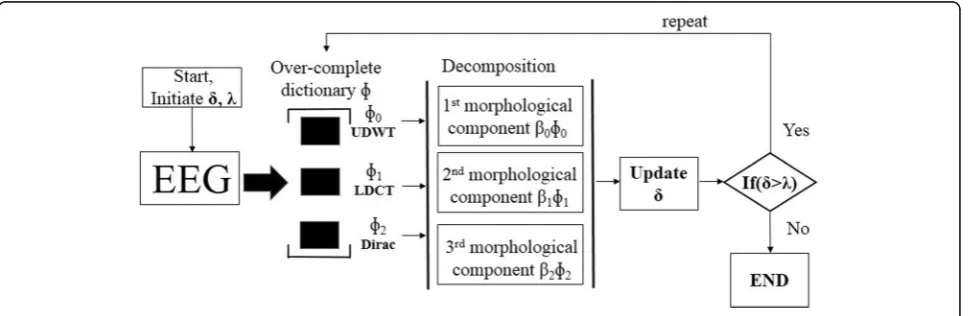
The number of iteration Imax=100 is used. Balbir et al.

[39] had varied the value of λfrom 3 to 5 depending on the type of hard and soft threshold. In this work, λ= 3 is used. Figure1depicts the working of MCA as described in Algorithm 1. From Figs. 2 and3, it can be observed that

UDWT is showing slow component of EEG whereas LDCT showing spectral component. Dirac basis is showing its ability to capture the spike morphology of EEG, captur-ing the negative spike train of seizure or ictal in Fig.3.

4 Hilbert transform over decompositions

Hilbert transform was applied to the components pro-duced by MCA. Representing real valued componentc(t) into analytic form s(t) onto the real axis of the complex domain as

s tð Þ ¼c tð Þ þjcHð Þt ; ð4Þ

Hilbert transform over c(t) produce cH(t). The

analyt-ical form signifies that there is a shift or phase difference

of π₂ between the positive and the negative frequency.

Imaginary part representing negative frequency is ignored, and only the real part representing the positive frequency is considered for working due to Hermitian symmetry. Equation (4) can be represented as in [19]

s tð Þ ¼a tð Þejφð Þt ð5Þ

Instantaneous phase φ(t) and amplitude a(t) can be given by

φð Þ ¼t arctan cHð Þt c tð Þ

: ð6Þ

a tð Þ ¼

ffiffiffiffiffiffiffiffiffiffiffiffiffiffiffiffiffiffiffiffiffiffiffiffiffiffiffi

c2ð Þ þ_{t c}2

Hð Þt ;

q

ð7Þ

Instantaneous frequency is defined as derivative of instantaneous phase as in [49]

ωð Þ ¼t φ0ð Þt : ð8Þ

Prime is representing differentiation in this work.

5 Computation of root mean instantaneous frequency square

Equation (9a) can be expressed in another way by using

Hermitian time frequency operator ð1

jdtdÞ . Center

frequency can be written as in [50]

<ω>¼

Z

ωjSð Þω j2dω; ð9aÞ

¼

Z

sð Þt 1 j

d

dts tð Þdt; ð9bÞ

¼

Z φ0

t ð Þ þ1

j a0ð Þt a tð Þ

a2ð Þt dt; ð9cÞ

<ω>¼

Z φ0

t

ð Þa2ð Þt dt; ð9dÞ

Imaginary part is ignored as zero, s∗(t) is complex conjugate signal, anda2(t) is density in time [51].

Therefore, center frequency, as in [50], can be given by

<ω>¼

Z φ0

t

ð Þa2ð Þt dt; ð10Þ

TheS(ω) is the Fourier transform of the signals(t).

Sð Þ ¼ω 1ffiffiffi 2 p

Z

e−iωt_{s tð Þdt: ð11Þ}

Amplitude is normalized, and using Parseval’s theorem, ∫|S(ω)|2dω=∫|s(t)|2dt= 1. All integrals computed are be-tween time interval [0, 23.6] as EEG signal segments [52] used in this work is of 23.6 s as described in Section7.

By referring to [51, 53], when time-averaged square

bandwidth σ2

T also known as bandwidth frequency

modulation (BFM) [51] is expanded, this can be

repre-sented as in Eq. (12b). Rearranging Eq. (12b) gives us a root mean instantaneous frequency square (RMIFS) frequency. <.>Tmeans time domain.

σ2

T¼

Z φ0

t

ð Þ−<ω>

ð Þ2

a2ð Þdtt ; ð12aÞ

σ2

T¼<φ

02

t

ð Þ>−<ω>2_{; ð12bÞ}

σ2

T¼<ω2>−<ω>2; ð12cÞ

<ω2_>¼σ2

Tþ<ω>2; ð12dÞ

fR¼

ffiffiffiffiffiffiffiffiffiffiffiffiffiffiffiffiffiffiffiffiffiffiffiffiffi σ2

Tþ<ω>2

q

: ð12eÞ

σ2

T and <ω>

2

are parameters, as can be seen in Eq. (12d), and their ratio can be given by

EMIFS¼<ω> 2

σ2

T

: ð13Þ

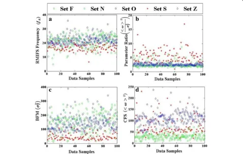
Features extracted from components are depicted in Table1and in Fig.4.

6 SVM

Support vector machine (SVM), introduced by Vapnik [54], is used as classifier. SVM discriminate two different classes by creating a hyperplane which maximizes

distance between among them. Radial basis function (RBF) kernel is used in this work represented:

G xi;xj

¼ exp

xi;−x j

k k2 2σ2

; ð14Þ

whereσis a positive number.

7 Dataset

EEG dataset [52] commonly known as Bonn dataset

was used to apply the method. Five subsets F, N, O, S, and Z make the dataset. All subsets consist of 100 signal segments, each of 23.6 s duration recorded with 173.61 Hz of sampling frequency containing 4097 samples. Subsets O and Z are recorded extracra-nially with eye open and with eyes closed from healthy subjects having no previous seizure history. Subsets F, N, and S have signal segments from intra-cranial experiments. Subsets F and N have interictal recording. Subset N is from the epileptic zone, and F is from the hippocampal formation of the opposite hemisphere. Subset S contains ictal EEG recording. In this work, six combinations of subsets are created for

Table 1Feature extracted from components

Feature UDWT LDCT Dirac

fR ✓

EMIFS ✓

σ2

T ✓

<ω>2 ✓

Fig. 4FeaturesaRMIFS frequency from Dirac component.bParameters ratio (<ω_σ2>2

T

) from Dirac component.cBandwidth frequency modulation

classification. First one is with sets F, S, second with N, S, third with O against S, fourth with Z against S, fifth with F, N together versus S, and sixth with O, Z against S for classification.

Every subset contains 100 data from each feature calculated upon 100 signal segments. These data are normalized using standard deviation and mean. Training and test set are prepared in 70:30 ratio for SVM. For one subset versus another individual subset’s classifica-tion, 70 samples are picked randomly without replace-ment from each set to create training set. Test set is made from the remaining 30 data samples. For F, N ver-sus S, 35 samples are taken randomly without re-placement from each F, N subsets and 70 random samples were picked without replacement from S set to make SVM training set. For test set, 15 samples are picked randomly from remaining 65 data samples from the subsets F, N and 30 remaining samples are taken from S set. The step of picking equal number of data samples from interictal and ictal sets was taken to avoid any bias and overfitting. Same process was adapted for classification of O, Z against S. Using grid search, best kernel parameters were searched, i.e., similar to cross-validation. But in most of the case, default kernel parameters have shown good results as

presented in Table 2. We repeated this process

hun-dred times means taking 100 trials following Bajaj et al. [23] who has taken 10 trials.

8 Simulation

In MCA methodology, sparsity play a vital role in separating the components having different time-frequency properties or morphology of constructing of individual source components. The combination of explicit dictionaries forming an over-complete diction-ary makes the MCA more powerful methods for

denoising and source component separation [39].

Mostly, decomposition-based methods like PCA and ICA required prior knowledge about the decomposed components. MCA-based decomposition has an advan-tage in the accurate reconstruction of the original com-ponent because the source comcom-ponent has a low probability of occurrence simultaneously. This method relies on the sparsity and the over-completeness of the dictionaryΦ ∈Rn×k, a set ofkredundant transforms, which represent the specific morphologies of different components of signal. Due to the concept of sparsity and the over-completeness, the dictionary extended the traditional signal decomposition to feature extractions of multiple types of morphology simultaneously. EEG signal contains specific morphology depending on the activity in the brain. Therefore, EEG time course data can be decomposed by one explicit dictionary and cannot be decomposed by other explicit dictionaries. It estimates the components accurately as the

decom-posed components are sparse and independent. The S

is the linear combination of different brain activity,

Table 2Classification results from 100 trials on all six combinations of subsets Feature RBF kernel parameters SPE [%]

where β is the brain activity and is the mixing matrix. Different basis functions were trialed in differ-ent combinations to create the epileptic-specific dic-tionary from a set of UDWT, discrete sine transform (DST), discrete cosine transform (DCT), LDCT, and Dirac basis functions, and finally, UDWT, LDCT, and Dirac were used depending on the significant differ-ence shown by the extracted, proposed features. UDWT has not been used directly for feature extrac-tion but has been kept in the dicextrac-tionary to make

LDCT spectral component remain free from

slow-moving components. Dirac basis was used to capture the spike morphology of the epileptic seizure. Dirac basis is also useful in capturing the transient spikes in interictal which can help in localizing the epileptic zone.

After using MCA for decomposition, Hilbert trans-form was applied over the components which take the real value signal decomposition to complex time fre-quency domain. Real signal gives symmetrical density in frequency making mean or center frequency zero. Using analytic representation, we will have identical spectrum for positive frequencies and zero for negative frequencies [50]. Feature RMIFS (fR) and the parameters ratio (<ω>

2 σ2

T

)

are computed from Dirac component. RMIFS is defined as root over sum of the time-averaged bandwidth square

σ2

T and the center frequency square <ω>

2

. f2R is always

greater than <ω>2by σ2

T. This feature is expressed

com-pletely in terms of frequency modulationσ2

T and average

or center frequency square <ω>2in time domain which is advantageous as it is free from any amplitude-based component that is prone to noise. ComputingfRdirectly

as pffiffiffiffiffiffiffiffiffiffiffiffiffiffiffiffiffiffiffiffiffiffi<φ02_{ðtÞ> or as} ffiffiffiffiffiffiffiffiffiffiffiffiffiffiffiffiffiffiffiffiffiffiffiffiffi_σ2

Tþ<ω>2

p

gives same value. The parameters ratio (<ω_σ2>2

T ) shows how dominant center

frequency square is over time-averaged bandwidth square. For example, from Fig.4c, in the case of interic-tal σ2

T is at higher range making the parameters ratio at

lower range whereas for ictal the behavior is opposite means during the ictal event, the frequency modulation is small compared to interictal as also observed by Bajaj et al. [23]. Frequency modulationσ2

T from Dirac

compo-nent is at higher range in nonseizure and interictal than ictal, and center frequency from LDCT component is highest in nonseizure than in ictal and lowest in interic-tal. As time-averaged bandwidth can be taken as the standard deviation of instantaneous frequency around the center frequency and center frequency as the

mean, fR satisfies the definition of root mean square.

Value of _fR will be close to center frequency when

in-stantaneous frequencies are close to center frequency leading to smallσ2_T. That is, signal decomposition during epileptic event showing small frequency modulation will

result in f2R influenced by center frequency square <ω>

2 . Dirac component was chosen for computation of RMIFS frequency because, firstly, it represents the spike morph-ology of the EEG and, secondly, it shows more

signifi-cant difference than when fR is computed from LDCT

component. For classification using <ω>2and σ2_T, <ω>2

is computed from LDCT component and σ2_T from Dirac

component simultaneously because LDCT represents the frequency component better than Dirac which shows modulation better.

Center frequency square <ω>2 calculated from LDCT component are in range from higher delta wave to lower alpha wave in interictal sets F, N, whereas in healthy nonseizure sets O, Z, it is between higher theta wave to alpha wave. Center frequency in ictal set S was dispersed

between lower theta wave to lower beta wave. RMIFSfR

on an average is in beta range for all the subsets of the Bonn dataset as presented in Fig.4.

9 Results and discussion

These features are normalized using mean and standard deviation then fed to SVM in a set of two pairs separ-ately to elaborate its significance in classification of seizures. These pairs of features are selected as they are showing opposite behavior which helps SVM to create the hyperplane discriminating the classes. Performance of the SVM classifier is evaluated by using the statistical parameters from previous works, i.e., specificity (SPE), sensitivity (SEN), and accuracy (Acc) [4,23].

SPE¼ TN

where true positive and true negative events are denoted by TP and TN, i.e., detecting ictal and interictal cor-rectly. FN and FP stands for false negative and false posi-tive, respectively.

Classification of result of set F versus set S using both pairs of feature, i.e.,fR, (<ω> lar result of average accuracy of 96.48 and 97.13% and average sensitivity of 93.53 and 94.26%. Average specifi-city using both the features are very high at 99.43 and 100.0%. Results are shown in Table2.

Classification accuracy of both the pairs of feature for set N against S is good at 99.41 and 99.48%. Average sensitivity and specificity are 99.46, 99.90, 99.36, and 99.66%. For set O versus Z, featuresfR, (<ω>

2 σ2

T ) show

Fig. 5Set N vs S classification using RBF kernelσ= 1.0,c= 1.0. 0 (Ictal Training); 1 (Interictal Training); Support Vectors; SVM Hyperplane; 0 (Ictal Classified); and 1 (Interictal Classified)

87.98%. Similar accuracy result is observed for set Z ver-sus S with 99.63% usingfR, (<ω>

2 σ2

T

), whereas 90.30% using

σ2

T, <ω>

2

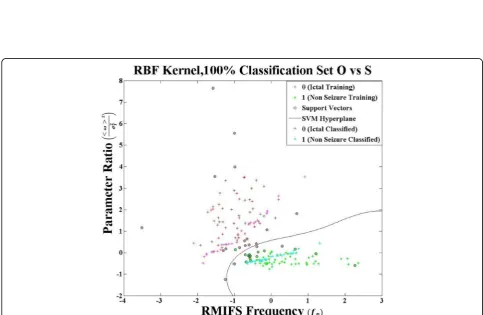
. SVM plot for set N versus S using σ2

T, <ω>

2

and set O against S using fR, (<ω>

2 σ2

T ) is shown in Figs.5

and 6. Average accuracy for set F, N together versus set S are at 93.05 and 93.61% for both sets of features, whereas average classification accuracy for set O, Z ver-sus S are at 99.11 and 90.60%. We have compared this proposed work with previous work at Tables3and4.

For most of the time default kernel parameters proved to be better. Even with an optimized parameters that are found with grid search, were close to default setting and shows little improvement of at most 1–1.5%. Therefore, the cases where we found improvement less than 1%, default setting or default kernel parameters were used which helped in avoiding computing overload of kernel parameters search and makes the application more prac-tical. Both the pairs of features have shown similar clas-sification result for interictal set versus ictal or seizure

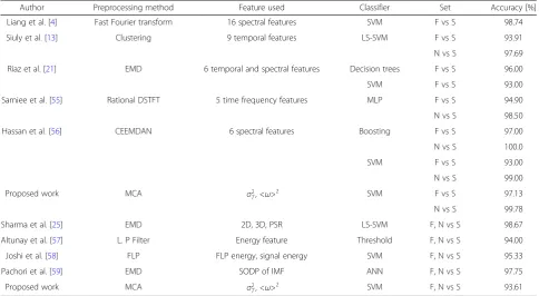
Table 3Comparison of set F, N vs S results with other existing works on Bonn dataset

Author Preprocessing method Feature used Classifier Set Accuracy [%]

Liang et al. [4] Fast Fourier transform 16 spectral features SVM F vs S 98.74

Siuly et al. [13] Clustering 9 temporal features LS-SVM F vs S 93.91

N vs S 97.69

Riaz et al. [21] EMD 6 temporal and spectral features Decision trees F vs S 96.00

SVM F vs S 93.00

Samiee et al. [55] Rational DSTFT 5 time frequency features MLP F vs S 94.90

N vs S 98.50

Hassan et al. [56] CEEMDAN 6 spectral features Boosting F vs S 97.00

N vs S 100.0

SVM F vs S 93.00

N vs S 99.00

Proposed work MCA σ2

T, <ω>

2 _{SVM F vs S 97.13}

N vs S 99.78

Sharma et al. [25] EMD 2D, 3D, PSR LS-SVM F, N vs S 98.67

Altunay et al. [57] L. P Filter Energy feature Threshold F, N vs S 94.00

Joshi et al. [58] FLP FLP energy, signal energy SVM F, N vs S 95.33

Pachori et al. [59] EMD SODP of IMF ANN F, N vs S 97.75

Proposed work MCA _σ2

T, <ω>

2 _{SVM F, N vs S 93.61}

RDSTFTrational discrete STFT,CEEMDANcomplete ensemble empirical mode decomposition with adaptive noise,PSRphase space representation,L. P Filterlinear

prediction filter,FLPfractional linear prediction

Table 4Comparison with other works on Bonn dataset for classification between healthy nonseizure set O, Z and seizure or ictal set S

Author Preprocessing method Feature used Classifier Set Accuracy [%]

Guo et al. [10] Genetic algorithm Curve length, standard deviation KNN Z vs S 99.20

Siuly et al. [13] Clustering 9 temporal features LS-SVM Z vs S 99.90

O vs S 96.30

Samiee et al. [55] Rational DSTFT 5 time frequency features MLP Z vs S 99.80

Hassan et al. [56] CEEMDAN 6 spectral features Boosting Z vs S 100.0

Rincon et al. [60] Wavelet transform Bag of words SVM Z vs S 99.85

Wavelet coefficient SVM Z vs S 100.0

Proposed work MCA fR,EMIFS SVM Z vs S 99.63

O vs S 99.91

Chen et al. [11] DTCWT Logarithm of FFT spectra NN Z, O vs S 100

Proposed work MCA fR,EMIFS SVM Z, O vs S 99.11

set whereas feature fR, (<ω>

2 σ2

T

) has shown better results

for healthy nonseizure classification against seizure set. Therefore,fR, (<ω>

2 σ2

T ) features combination for

classifica-tion are found to better than σ2

T, <ω>

2

. Figure4clearly shows it is hard to have two-dimensional map helping SVM to create hyperplane to separate nonseizure and seizure sets using feature combination of σ2_T, <ω>2as they are quite intermingled. Although classification of seizure set which is the result of intracranial experiment against noninvasive extracranial nonseizure healthy EEG set is inappropriate, classification has been done for comparison purpose of the proposed method with previ-ous works. Detailed comparison of the proposed work with the previously done work on Bonn dataset is pre-sented in Tables3and4.

10 Conclusions

MCA gives definite number of decomposition depend-ing on the number of set of basis used in over-complete dictionary. This dictionary can be formed based on problem requirements. Selection of basis functions in the dictionary plays an important role in creating problem-specific application. We found LDCT component is best suited for spectral feature extraction, whereas Dirac bases are good in showing spike morph-ology of the EEG. Default setting of SVM kernel is suit-able for proposed feature combinations which makes it suitable for practical application. To make the method reliable, 100 random trials were taken on SVM. 99.78% of highest average accuracy was observed for classifica-tion of interictal set N against ictal set S, whereas 99.91% of average accuracy was observed for classifica-tion of nonseizure set O against ictal set S. In future, we will try to form a dictionary to remove different arti-facts from EEG and will try to create seizure prediction system using MCA and proposed features with suitable basis for long-term EEG signals.

Abbreviations

Acc:Accuracy; ApEn: Approximate entropy; BCR: Block coordinate relaxation; BFM: Bandwidth frequency modulation; CEEMDAN: Complete ensemble empirical mode decomposition with adaptive noise; CFS: Center frequency square; DCT: Discrete cosine transform; DST: Discrete sine transform; DTCWT: Dual tree complex wavelet; EEG: Electroencephalogram; EMD: Empirical mode decomposition; FFT: Fast Fourier transform; FLP: Fractional linear prediction; FN: False negative; FP: False positive; ICA: Independent component analysis; IMF: Intrinsic mode function; KNN: K nearest neighbor; L.P Filter: Linear prediction filter; LDCT: Local discrete cosine transform; LS-SVM: Least square support vector machine; MCA: Morphological component analysis; MLP: Multilayer perceptron; NN: Nearest neighbor; PC: Principal component; PCA: Principal component analysis; PSR: Phase space representation; RBF: Radial basis function; RDSTFT: Rational discrete STFT; RMIFS: Root mean instantaneous frequency square; SEN: Sensitivity; SPE: Specificity; STFT: Short-time Fourier transform; SVM: Support vector machine; TN: True negative; TP: True positive; UDWT: Undecimated wavelet transform

Availability of data and materials

The EEG dataset [52] used in this work is available athttp:// www.meb.unibonn.de/epileptologie/science/physik/EEGdata.html

Authors’contributions

The MCA code developed by Dr. BS under the supervision of Dr. HW is used in this work. Selection of basis function to create dictionary for epileptic application, feature proposal and extraction, classification and result analysis is done by AGM under the supervision of Dr. KH. All authors read and approved the final manuscript.

Ethics approval and consent to participate

Not applicable.

Consent for publication

Not applicable.

Competing interests

The authors declare that they have no competing interests.

Publisher’s Note

Springer Nature remains neutral with regard to jurisdictional claims in published maps and institutional affiliations.

Author details

1_{Graduate School of Life Science and Systems Engineering, Kyushu Institute}

of Technology, Kitakyushu, Japan.2_{National Institute for Physiological}

Sciences, Okazaki, Japan.3Artificial Intelligence Research Center, National Institute of Advanced Industrial Science and Technology, Tokyo, Japan.

4_{Riken BSI, Wako, Japan.}

Received: 18 January 2018 Accepted: 18 June 2018

References

1. RS Fisher, WE Boas, W Blume, C Elger, P Genton, P Lee, J Engel, Epileptic seizures and epilepsy: definitions proposed by the international league against epilepsy (ilae) and the international bureau for epilepsy (ibe). Epilepsia46(4), 470–472 (2005)

2. AT Berg, SF Berkovic, MJ Brodie, J Buchhalter, JH Cross, WE Boas, J Engel, J French, TA Glauser, GW Mathern, et al., Revised terminology and concepts for organization of seizures and epilepsies: report of the ILAE commission on classification and terminology, 2005-2009. Epilepsia

51(4), 676–685 (2010)

3. S Ramgopal, S Thome-Souza, M Jackson, NE Kadish, IS Fernandez, J Klehm, W Bosl, C Reinsberger, S Schachter, T Loddenkemper, Seizure detection, seizure prediction, and closed-loop warning systems in epilepsy. Epilepsy Behav.37, 291–307 (2014)

4. SF Liang, HC Wang, WL Chang, Combination of EEG complexity and spectral analysis for epilepsy diagnosis and seizure detection. EURASIP J. Adv. Signal Process.2010(1), 853434 (2010)

5. V Srinivasan, C Eswaran, N Sriraam, Artificial neural network based epileptic detection using time-domain and frequency-domain features. J. Med. Syst.

29(6), 647_–660 (2005)

6. K Polat, S Günes, Classification of epileptiform EEG using a hybrid system based on decision tree classifier and fast Fourier transform. Appl. Math. Comput.187(2), 1017–1026 (2007)

7. AT Tzallas, MG Tsipouras, DI Fotiadis, Epileptic seizure detection in EEGs using time-frequency analysis. IEEE Trans. Inf. Technol. Biomed.13(5), 703– 710 (2009)

8. H Adeli, Z Zhou, N Dadmehr, Analysis of EEG records in an epileptic patient using wavelet transform. J. Neurosci. Methods123(1), 69_–87 (2003) 9. H Ocak, Optimal classification of epileptic seizures in EEG using wavelet

analysis and genetic algorithm. Signal Process.88(7), 1858–1867 (2008) 10. L Guo, D Rivero, J Dorado, AP CR Munteanu, Automatic feature extraction

using genetic programming: an application to epileptic EEG classification. Expert Syst. Appl.38(8), 10425–10436 (2011)

11. G Chen, Automatic EEG seizure detection using dual-tree complex wavelet-Fourier features. Expert Syst. Appl.41(5), 2391–2394 (2014)

13. Y Li, PP Wen, et al., Clustering technique-based least square support vector machine for EEG signal classification. Comput. Methods Prog. Biomed.

104(3), 358–372 (2011)

14. Z Iscan, Z Dokur, T Demiralp, Classification of electroencephalogram signals with combined time and frequency features. Expert Syst. Appl.38(8), 10499–10505 (2011)

15. Y Tang, D Durand, A tunable support vector machine assembly classifier for epileptic seizure detection. Expert Syst. Appl.39(4), 3925_– 3938 (2012)

16. N Nicolaou, J Georgiou, Detection of epileptic electroencephalogram based on permutation entropy and support vector machines. Expert Syst. Appl.

39(1), 202–209 (2012)

17. G Zhu, Y Li, PP Wen, Epileptic seizure detection in EEGs signals using a fast weighted horizontal visibility algorithm. Comput. Methods Prog. Biomed.

115(2), 64–75 (2014)

18. A Temko, E Thomas, W Marnane, G Lightbody, G Boylan, EEG-based neonatal seizure detection with support vector machines. Clin. Neurophysiol.122(3), 464_–473 (2011)

19. NE Huang, Z Shen, SR Long, MC Wu, HH Shih, Q Zheng, NC Yen, CC Tung, HH Liu, inProceedings of the Royal Society of London A: Mathematical, Physical and Engineering Sciences, the Royal Society. The empirical mode decomposition and the Hilbert spectrum for nonlinear and non-stationary time series analysis, vol 454 (1998), pp. 903_–995

20. RJ Oweis, EW Abdulhay, Seizure classification in EEG signals utilizing Hilbert-Huang transform. Biomed. Eng. Online10(1), 38 (2011)

21. F Riaz, A Hassan, S Rehman, IK Niazi, K Dremstrup, EMD-based temporal and spectral features for the classification of EEG signals using supervised learning. IEEE Trans. Neural Syst. Rehabil. Eng.24(1), 28–35 (2016) 22. F K, Q J, Y Chai, Y Dong, Classification of seizure based on the

time-frequency image of EEG signals using HHT and SVM. Biomed. Signal Process. Control13, 15_–22 (2014)

23. V Bajaj, RB Pachori, Classification of seizure and nonseizure EEG signals using empirical mode decomposition. IEEE Trans. Inf. Technol. Biomed.16(6), 1135_–1142 (2012)

24. AG Mahapatra, K Horio, inSystems, Man, and Cybernetics (SMC), 2016 IEEE International Conference on, IEEE. Overcoming drawback of feature instantaneous bandwidth using EMD for epileptic seizure classification by RMS frequency (2016), pp. 001322–001327

25. R Sharma, RB Pachori, Classification of epileptic seizures in EEG signals based on phase space representation of intrinsic mode functions. Expert Syst. Appl.42(3), 1106–1117 (2015)

26. K Samiee, P Kovacs, M Gabbouj, Epileptic seizure detection in long-term EEG records using sparse rational decomposition and local Gabor binary patterns feature extraction. Knowl.-Based Syst.118, 228–240 (2017) 27. J Spilka, J Frecon, R Leonarduzzi, N Pustelnik, P Abry, M Doret, Sparse

support vector machine for intrapartum fetal heart rate classification. IEEE J. Biomed. Health Inform.21(3), 664_–671 (2017)

28. IJ Rampil, A primer for EEG signal processing in anesthesia. Anesthesiology

89(4), 980–1002 (1998)

29. B Crepon, V Navarro, D Hasboun, S Clemenceau, J Martinerie, M Baulac, C Adam, M Le Van Quyen, Mapping interictal oscillations greater than 200 Hz recorded with intracranial macroelectrodes in human epilepsy. Brain133(1), 33_–45 (2009)

30. HS Liu, T Zhang, FS Yang, A multistage, multimethod approach for automatic detection and classification of epileptiform EEG. IEEE Trans. Biomed. Eng.49(12), 1557–1566 (2002)

31. KJ Blinowska, PJ Durka, Unbiased high resolution method of EEG analysis in time-frequency space. Acta Neurobiol. Exp.61(3), 157{174 (2001) 32. E Imani, HR Pourreza, T Banaee, Fully automated diabetic retinopathy

screening using morphological component analysis. Comput. Med. Imaging Graph.43, 78_–88 (2015)

33. E Imani, M Javidi, HR Pourreza, Improvement of retinal blood vessel detection using morphological component analysis. Comput. Methods Prog. Biomed.118(3), 263_–279 (2015)

34. A Hyvärinen, E Oja, Independent component analysis: algorithms and applications. Neural Netw.13(4–5), 411–430 (2000)

35. P Berg, M Scherg, A multiple source approach to the correction of eye artifacts. Electroencephalogr. Clin. Neurophysiol.90(3), 229–241 (1994) 36. GL Wallstrom, RE Kass, A Miller, JF Cohn, NA Fox, Automatic correction of

ocular artifacts in the EEG: a comparison of regression-based and component-based methods. Int. J. Psychophysiol.53(2), 105–119 (2004)

37. A Hyvärinen, J Särelä, R Vigario, inProc. Int. Workshop on Independent Component Analysis and Signal Separation (ICA'99). Spikes and bumps: Artefacts generated by independent component analysis with insu cient sample size (1999), pp. 425–429

38. J Särelä, R Vigario, Overlearning in marginal distribution based ica: analysis and solutions. J. Mach. Learn. Res.4(Dec), 1447_–1469 (2003)

39. B Singh, H Wagatsuma, A removal of eye movement and blink artifacts from EEG data using morphological component analysis. Comput. Math. Methods Med.2017, 1861645 (2017)

40. Y Jiang, M Wang, Image fusion with morphological component analysis. Inf. Fusion18, 107–118 (2014)

41. M Dalla Mura, A Villa, JA Benediktsson, J Chanussot, L Bruzzone, Classification of hyperspectral images by using extended morphological attribute profiles and independent component analysis. IEEE Geosci. Remote Sens. Lett.8(3), 542–546 (2011)

42. RK X Yong, GE Ward, inNeural Engineering, 2009. NER'09. 4th International IEEE/EMBS Conference on, IEEE. Birch, generalized morphological component analysis for EEG source separation and artifact removal (2009), pp. 343_–346 43. S JW Matiko, J Beeby, inEngineering in Medicine and Biology Society (EMBC), 2013 35th Annual International Conference of the IEEE, IEEE. Tudor, real time eye blink noise removal from EEG signals using morphological component analysis (2013), pp. 13_–16

44. SS Chen, DL Donoho, MA Saunders, Atomic decomposition by basis pursuit. SIAM Rev.43(1), 129–159 (2001)

45. M Püschel, JM Moura, The algebraic approach to the discrete cosine and sine transforms and their fast algorithms. SIAM J. Comput.32(5), 1280{1316 (2003)

46. X Shao, SG Johnson, Type-IV DCT, DST, and MDCT algorithms with reduced numbers of arithmetic operations. Signal Process.88(6), 1313–1326 (2008) 47. Y JL Starck, J Moudden, M Bobin, DD Elad, Morphological component

analysis. Proc. SPIE5914, 1–15 (2005)

48. S Sardy, A Bruce, P Tseng, Block coordinate relaxation methods for nonparametric signal denoising with wavelet dictionaries, (1998). 49. PJ Loughlin, B Tacer, Comments on the interpretation of instantaneous

frequency. IEEE Signal Process Lett.4(5), 123–125 (1997)

50. L Cohen,Time-frequency analysis(Prentice Hall PTR, Englewood Cliffs, 1995) 51. L Cohen, C Lee, inAcoustics, Speech, and Signal Processing, 1990. ICASSP-90., 1990 International Conference on, IEEE. Instantaneous bandwidth for signals and spectrogram (1990), pp. 2451–2454

52. RG Andrzejak, K Lehnertz, F Mormann, C Rieke, P David, CE Elger, Indications of nonlinear deterministic and finite-dimensional structures in time series of brain electrical activity: dependence on recording region and brain state. Phys. Rev. E64(6), 061907 (2001)

53. S Tolwinski,The Hilbert Transform and Empirical Mode Decomposition as Tools for Data Analysis(University of Arizona, Tucson, 2007)

54. V Vapnik,The nature of statistical learning theory(Springer science & business media, 2013)

55. K Samiee, P Kovacs, M Gabbouj, Epileptic seizure classification of EEG time-series using rational discrete short-time Fourier transform. IEEE Trans. Biomed. Eng.62(2), 541_–552 (2015)

56. AR Hassan, A Subasi, Automatic identification of epileptic seizures from EEG signals using linear programming boosting. Comput. Methods Prog. Biomed.136, 65–77 (2016)

57. S Altunay, Z Telatar, O Erogul, Epileptic EEG detection using the linear prediction error energy. Expert Syst. Appl.37(8), 5661–5665 (2010) 58. V Joshi, RB Pachori, A Vijesh, Classification of ictal and seizure-free EEG

signals using fractional linear prediction. Biomed. Signal Process. Control9, 1_–5 (2014)

59. RB Pachori, S Patidar, Epileptic seizure classification in EEG signals using second-order difference plot of intrinsic mode functions. Comput. Methods Prog. Biomed.113(2), 494–502 (2014)