R E S E A R C H
Open Access
Stationary time-vertex signal processing
Andreas Loukas
1*†and Nathanaël Perraudin
2†Abstract
This paper considers regression tasks involving high-dimensional multivariate processes whose structure is dependent on some known graph topology. We put forth a new definition of time-vertex wide-sense stationarity, orjoint
stationarityfor short, that goes beyond product graphs. Joint stationarity helps by reducing the estimation variance and recovery complexity. In particular, for any jointly stationary process (a) one reliably learns the covariance structure from as little as a single realization of the process and (b) solves MMSE recovery problems, such as interpolation and denoising, in computational time nearly linear on the number of edges and timesteps. Experiments with three datasets suggest that joint stationarity can yield accuracy improvements in the recovery of high-dimensional processes evolving over a graph, even when the latter is only approximately known, or the process is not strictly stationary.
Keywords: Stationarity, Multivariate time-vertex processes, Harmonic analysis, Graph signal processing, PSD estimation
1 Introduction
One of the main challenges when modeling multivari-ate processes is to decouple the estimation variance from the problem size. Consider anN-variate process unfold-ing overTtimesteps. If only mild assumptions are made, then the number of realizations needed to reliably esti-mate the first two moments is up to a logarithmic factor proportional toO(NT), i.e., the data size [1]. Assuming that the process is time wide-sense stationarity (TWSS) makes the lengthT of the process inconsequential. This is ideal for the univariate setting as it enables us to make relevant predictions even based on a single realization. If one additionally assumes that the signal autocorrelation is compactly supported, such that most data dependencies take place within a short time horizon, then the estima-tion variance can be reduced further by (roughly) splitting the observations into parts and considering each as an independent realization. This approach suffices whenNis relatively small. For high-dimensional processes, however, one needs to incorporate additional assumptions to obtain meaningful predictions [2–5].
In this spirit, this paper focuses on high-dimensional processes that are supported on the vertex set and are
*Correspondence:[email protected]
†Andreas Loukas and Nathanaël Perraudin contributed equally to this work. 1Laboratoire de Traitement des Signaux 2, École Polytechnique Fédérale Lausanne, 1015 Lausanne, Switzerland
Full list of author information is available at the end of the article
statistically dependent on the edge set of some known graph topology. Whether examining epidemic spreading [6], how traffic evolves in the roads of a city [7], or neu-ronal activation patterns present in the brain [8], many of the high-dimensional processes one encounters are inherently constrained by some underlying network. This realization has been the driving force behind recent efforts to re-invent classical models by taking into account the graph structure, with advances in many problems, such as denoising [9] and semi-supervised learning [10, 11], among others.
Yet, standard models for processes (evolving) on graphs often fail to produce useful results when applied to real datasets. One of the main reasons for this shortcoming is that they model only a limited set of spatiotemporal behaviors. The well-used graph Tikhonov and total variation priors, for instance, assume that the signal varies slowly or in a piece-wise constant manner over edges, without specifying any precise relations [12–14]. Similarly, assuming that the graph Laplacian encodes the conditional correlations of variables, as is done with Gaussian Markov random fields [15], becomes a rigid model when the graph is known [16]. To capture the behavior of complex networked systems, such as trans-portation and biological networks, it is crucial to train expressive models, being able to reproduce a wide range of graph and temporal behaviors.
1.1 Contributions
This paper considers the statistical modeling of processes evolving on graphs. In particular, we investigate the rela-tionship between two different hypotheses: TWSS and VWSS [17–19], which are individually helpful in reduc-ing the variance of covariance estimation for time series and graph signals, respectively. We propose a combined multivariate hypothesis that we refer to as time-vertex wide-sense stationarity, orjoint stationarityfor short. The necessary first step of our analysis consists of reformu-lating the standard properties of stationarity (such as the relation of the covariance matrix and power spectral den-sity to an appropriate Fourier transform) from the lens of time-vertex analysis [20,21]. This analysis is purpose-ful, yet not trivial as joint stationarity is more complicated than assuming stationarity on the product of two graphs1. We use the hypothesis of joint stationarity to control variance and computational complexity in estimation and recovery tasks. Similar to [17], also here, one may reli-ably estimate the model parameters from few observations (e.g., see Fig. 4) and solve MMSE recovery problems in time linear on the number of edges and timesteps (e.g., see Fig.3). Complimenting previous work, we also provide an analysis of the power spectral density (PSD) estimation, which brings insight into the inherent trade-off between bias and variance. In addition, we experimen-tally demonstrate that assuming joint stationarity aids in recovery even when only an approximation of the graph is known, or the process is only approximately jointly stationary. These experiments corroborate that the joint stationarity hypothesis is a useful assumption, particularly in situations when the problem features a large number of variables but only a limited number of observations.
To test the utility of joint stationarity, we apply our methods on three diverse datasets: (a) a meteorological dataset containing the hourly temperature of 32 weather stations over 1 month in Molene, France [18], (b) a traffic dataset depicting high-resolution daily vehicle flow of 4 weekdays in the highways of Sacramento, and (c) simu-lated SIRS-type epidemics over Europe. Our experiments confirm that for high-dimensional processes evolving over graphs, assuming joint stationarity yields an improve-ment in recovery performance as compared to time- or vertex-based stationarity methods, even when the graph is only approximately known and the data violate the strict conditions of our definition.
1.2 Related work
There exists an extensive literature on multivariate sta-tionary processes, developing the original work of Wiener
1As it will be discussed in Section3.2, joint stationarity is strictly more general than vertex stationarity on the product of the two graphs (first proposed in [14] in the deterministic setting), as the latter can only model processes with specific PSD.
et al. [22,23]. The reader may find interesting Bloomfield’s book [24] focusing on spectral relations. We focus on two main approaches that relate to our work, graphical models and signal processing on graphs.
1.2.1 Graphical models
In the context of graphical models, multivariate station-arity has been used jointly with a graph in the work of [25,26]. Though relevant, we note that there is a key dif-ference of these models with our approach: we assume that the graph is given, whereas in graphical models, the graph structure (or more precisely the precision matrix) is learned from the data. Knowing the graph allows us to search for more involved relations between the variables. As such, we are not restricted to the case that the condi-tional dependencies are given by the graph (and therefore that they are sparse), but allow non-adjacent variables to be conditionally dependent, modeling a broader set of behaviors. We also note that our approach is even-tually more scalable. We refer to [16] for elements of connections between graphical models and graph signal processing.
1.2.2 Graph signal processing
The idea of studying the stationarity of a random vector w.r.t. a graph was first introduced in [18,27] and then in [17, 19]. While these contributions have different start-ing points, they both roughly propose the same definition. Another more recent contribution relating to stationarity on graphs in the context of PSD estimation is [28]. Despite the relevance of these works, it is important to stress that the current paper is the first to consider a stationary hypothesis over graph signals varying in time. Moreover, the new results are non-trivial as they cannot be obtained by applying previous definitions on a product graph. In addition, some of the analysis presented here (particularly that of Section4) is novel and can also be employed for the previously studied case of stationary graph signals. To make the connection with previous works transpar-ent, in the following, every technical result (e.g., Lemma, Theorem, Proposition) that emerges as a generalization of [18,19,27] contains a reference in its heading pointing to the former claim.
and provide a theoretical analysis of the bias and variance of the old and new PSD estimators. Additionally, we study the complexity of the proposed solution and evaluate its merit w.r.t. two new datasets.
2 Preliminaries
2.1 General notation
We use boldface symbols for matrices and vectors (e.g.,A andarespectively) and calligraphic symbols for sets (e.g.,
V andE). Symboljdenotes the imaginary unit,IN is the
N ×N identity matrix, and1N is the all-ones vector of
sizeN. We use brackets to index matrix elements and sub-scripts for matrix blocks: if A is of size n1× n2 , then A[n1,n2] is the element at then1th row andn2th column andAn1,n2 is a (block) matrix. Vectora = vec(A)
(with-out subscript) is the vectorized representation ofAandan
is itsnth column. Moreover, A is its transpose andA∗ is its transposed complex conjugate (meaning thatA∗T is the complex conjugate). IfAisN ×N Hermitian, its eigendecomposition is generically written asA=UU∗, whereU=[u1,. . .,uN] is a matrix having eigenvectors as
columns and=diag(λ1,. . .,λN)is the diagonal matrix
of eigenvalues. Symbolsh(·),f(·), andg(·)are reserved for scalar/matrix functions. A matrix function with a single argument takes as an input a symmetric matrix A and outputsh(A) = Udiag(h(λ1),. . .,h(λN))U. The
opera-tor⊗denotes the Kronecker product. The Kronecker sum
⊕can be defined in terms of the Kronecker product as A⊕B=A⊗IM+IN⊗B, where matrixBhas sizeM×M.
2.2 Harmonic time-vertex analysis
We consider signals supported on the vertices V =
{v1,v2,. . .,vN} of a weighted undirected graph G=
(V,E,WG), with E the set of edges of cardinality
E = |E| and WG the weighted adjacency matrix.
Suppose that signal xt is sampled at T successive
regu-lar intervals of unit length. A real time-vertex signalX= [x1,x2,. . .,xT]∈RN×T is then the matrix having graph
signalxtas itstth column.
The frequency representation of a time-vertex signalX is given by the joint Fourier transform [14,21] (or JFT for short)
ˆ
X=JFT{X}GFT{DFT{X}} =U∗GXU∗T, (1) with UG and UT being, respectively, the unitary graph
Fourier transform (GFT) and discrete Fourier transform (DFT) matrices, whereasU∗Tis the complex conjugate ofUT. In vector form, we have thatxˆ = JFT{x} U∗J x,
whereUJ =UT⊗UG. As is often the case, we chooseUG
to be the eigenvector matrix of the combinatorial2graph
2Though we use the combinatorial Laplacian in our presentation, our results can be adapted to alternative positive semi-definite matrix definitions of a graph Laplacian, such as the normalized Laplacian.
Laplacian matrixLG = diag(WG1N)−WG, where1N is
the all-ones vector of sizeN, and diag(WG1N)is the
diag-onal degree matrix. MatrixUT is the eigenvector matrix
of the LaplacianLTof a cyclic graphT: coefficient associated with the joint frequency [λn,ωτ],
whereλndenotes thenth graph eigenvalue andωτtheτth
angular frequency.
The JFT maintains a close connection with the prod-uct graph J [14, 21]. The latter is the graph whose adjacency matrix is WJ = WT ⊕ WG (this amounts
to a Cartesian product between G and the ring graph
T). The connection is revealed if one realizes that the LaplacianLJ = LT ⊕LG of J carries the
eigendecom-positionLJ = UJ(T ⊕G)UJ. It follows that
comput-ing the JFT (in vector form) is the same as computcomput-ing the GFT ofxw.r.t. graph J. The main issue with any3 product graph interpretation is that it imposes a strict dependence between the eigenvalues ofLGandLT (since
the eigenvalues of LJ are given by T ⊕ G). As we
will see in the next paragraph, to attain full generality, one needs to abandon the product graph. For an in-depth discussion of JFT and its properties, we refer the reader to [34].
2.3 Joint time-vertex filtering
Filtering a time-vertex signal x with a joint filter h(LG,LT)corresponds to element-wise multiplication in
the joint frequency domain [λ,ω] by a function h :
a diagonalNT×NTmatrix defined as
h(G,)=diag
and diag(vec(A))creates a matrix with diagonal elements the vectorized form ofA. The bi-variate notationh(·,·)is meant to illustrate that joint filters operateindependently
on the two domains, something impossible4 in the product graph framework [14,21]. For convenience, we will often overload notation and writeh(θn,τ) to refer to the bivariate functionh(λn,ωτ). Furthermore, we say that
a joint filter isseparable, if its joint frequency responseh can be written as the product of a frequency responseh1 defined solely in the vertex domain and oneh2in the time domain, i.e.,h(θ)=h1(λ)·h2(ω).
3 Joint time-vertex stationarity
Let X ∈ RN×T be a real discrete periodic multivariate stochastic process with a finite number of timesteps T that is indexed by the vertexviof graphGand timet. We
refer to such processes as time-vertex processes, orjoint processesfor short.
Our objective is to provide a definition of stationar-ity that captures statistical invariance of the first two moments of a joint processx = vec(X) ∼ D(x,¯ ), i.e., the meanx¯=E[x] and the covariance =E[xx]− ¯xx¯. Crucially, the definition should do so in a manner that is faithful to the graph and temporal structure.
3.1 Definition
Typically, wide-sense stationarity is thought of as an invariance of the two first moments of a process w.r.t. translation. For the first moment, things are straightfor-ward: stationarity implies a constant mean E[x] = c1, independently of the domain of interest. The second moment, however, is more complicated as it depends on the exact form translation takes in the particular domain. Unfortunately, for graphs, translation is a non-trivial oper-ation and three alternative transloper-ation operators exist: the generalized translation [37], the graph shift [13], and the isometric graph translation [27]. Due to this chal-lenge, there are currently three alternative (though akin) definitions of stationarity appropriate for graphs [17–19]. The ambiguity associated with translation on graphs urges us to seek an alternative starting point for our def-inition. Fortunately, there exists an interpretation which holds promise:up to its constant mean, a wide-sense sta-tionary process corresponds to a white process filtered linearly on the underlying space. This “filtering interpre-tation” of stationarity is well known classically5 as well as in the graph setting [19] and is equivalent to asserting that the second moment can be expressed as =h(LT),
whereh(LT)is a linear filter. Thankfully, not only
filter-ing is elegantly and uniquely defined for graphs [37], but
4Defining joint filters in terms of a product graph would imply that there is a fixed relation between angular and graph frequencies (determined by the product graph construction). As a result, in the product graph, framework filters are univariate functions.
5As the correlation between two instantst
1andt2depends only on the difference between these two instants
E[x[t1]x[t2]]−E[x[t1] ]E[x[t2] ]=γ[t1−t2], the covariance matrix has to be circulant, a property that is shared by linear filters.
also stating that a process is graph wide-sense stationary ifE[x]=c1Nand =h(LG), is a graph filter, is generally
consistent6with current definitions [17–19].
This motivates us to also express the definition of sta-tionarity for joint processes in terms of joint filtering:
Definition 1(JWSS)A joint processx=vec(X)is called jointly wide-sense stationary (JWSS), if and only if
(a) The first moment of the process is constant
E[x]=c1NT.
(b) The covariance matrix of the process is a joint filter
=h(LG,LT), whereh(·,·)is a non-negative real function referred to as joint power spectral density (JPSD).
Let us examine Definition1in detail.
First moment condition. As in the classical case, the first moment of a JWSS process has to be constant over the time and the vertex sets, i.e., X[i,¯ t]= c for every i=1, 2,. . .,Nandt=1, 2,. . .,T. For alternative choices of the graph Laplacian with a null-space not spanned by the constant vector, the first moment condition should be modified to requiring that the expected value of a JWSS process is in the null space of the matrixLT ⊕LG
(see Remark 2 [19] for a similar observation on stochastic graph signals).
Second moment condition.According to the definition, the covariance matrix of a JWSS process takes the form of a joint filterh(LG,LT), and is therefore diagonalizable by
the JFT matrixUJ. It may also be interesting to notice that
the matrixh(LG,LT)can be expressed as follows
must necessarily be positive-semidefinite; thus, h(·,·) is real (the eigenvalues of every Hermitian matrix are real) and non-negative. Also, equivalently, every zero mean JWSS processx = vec(X)can be generated by joint fil-tering x = h(LG,LT)1/2 a white process with zero
mean and identity covariance. The following proposition
6The only exception: for graphs with repeated eigenvalues, the conditions E[x]=c1and =h(LG)are sufficient but not necessary for the graph
exploits these facts to provide an interpretation of JWSS processes in the joint frequency domain.
Proposition 1(GeneralizesTheorem1 [17] andProposition 1 [18, 19])A joint process Xover a connected graph G is jointly wide-sense stationary (JWSS) if and only if:
(a) The joint spectral modes are in expectation zero
E
ˆ
X[n,τ]
=0 ifλn=0and ωτ =0.
(b) The product graph spectral modes are uncorrelated
E
ˆ
X[n1,τ1]X[nˆ 2,τ2]
=0,whenever
n1=n2orτ1=τ2.
(c) There exists a non-negative functionh(·,·), referred to as joint power spectral density (JPSD), such that
E
X[n,ˆ τ]2
−E
ˆ
X[n,τ]2=h(λn,ωτ),
for everyn=1, 2,. . .,Nandτ =1, 2,. . .,T.
(For clarity, this and other proofs of the paper have been moved to the “Appendix”.)
We briefly present a few additional properties of JWSS processes that will be useful in the rest of the paper.
Property 1 (Generalizes Example 1 [17–19])White centered i.i.d. noisew∈RNT∼D(0NT,INT)is JWSS with
constant JPSD for any graph.
The proof follows easily by noting that the covariance of wis diagonalized by the joint Fourier basis of any graph
w=I=UJIU∗J. This last equation tells us that the JPSD
is constant, which implies that similar to the classical case, the energy of white noise is evenly spread across all joint frequencies.
A second interesting property of JWSS processes is that stationarity is preserved through a filtering operation.
Property 2 (Generalizes Theorem 2 [17], Property 1 [19])When a joint filter f(LG,LT) is applied to a JWSS
process Xwith JPSD h, the resultY remains JWSS with mean cf(0, 0)1NT, where c is the mean of X, and JPSD
f2(λ,ω)h(λ,ω).
Finally, we notice that for real processesX, which are the focus of this paper, the functionhforming the joint fil-ter should be symmetric w.r.t.ω, meaning thath(λ,ω) = h(λ,−ω). This property can be easily derived from the definition of the Fourier transform.
3.2 Relations to classical definitions
We next provide an in-depth examination of the relations between joint wide-sense stationarity, time and vertex sta-tionarity, as well as their multivariate equivalents. For clar-ity, we order the rows/columns of the covariance matrix
such that each t1,t2 block of sizeN×Nmeasures the
covariance betweenxt1andxt2(see (4)).
3.2.1 Standard definitions
As we discuss below, known definitions of stationar-ity in time/vertex domains are particular cases of joint stationarity.
TWSS ∩VWSS ⊂ JWSS.The known versions of sta-tionarity (TWSS, VWSS) are oblivious to any structure along one of the two dimensions of X. In this man-ner, assuming that Xis TWSS amounts to interpreting each of theN time series as a separate realization of the sameprocess with TPSDhT(ω). Similarly, ifXis VWSS,
then each graph signal xt is taken as a separate
realiza-tion of asinglestochastic graph signal with VPSDhG(λ)
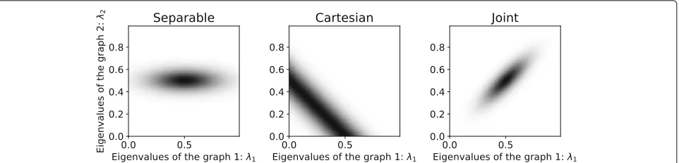
[17, 19]. It is a simple consequence that, different from the JWSS hypothesis, assuming thatXis both TWSS and VWSS is equivalent to limiting our scope to separable JPSD defined as the product of two univariate functions h(λ,ω)=hG(λ)hT(ω)—see also Fig.1.
3.2.2 Definitions based on the product graph
As explained in Section2, the JFT can be interpreted as a graph Fourier transform taken over a product graph whose Laplacian isLJ = LG⊕LT. This construction can
give rise to two additional definitions for joint stationarity:
VWSS on a product graph. The first is obtained by applying the VWSS definition of [17, 19] on the graph associated withLJ. The resulting model is not sufficiently
general in order to generate the full spectrum of JWSS processes. The reason is that, whereas the JPSDh(λ,ω) can be any two-dimensional non-negative function, the JPSD of any VWSS process on LJ is necessarily
one-dimensional (the eigenvalues of LJ are the sums of all
combinations of the eigenvalues ofLGandLT)—see Fig.1
for a pictorial demonstration and “Appendix:Univariate vs multivariate JPSD” for examples from real data. The same reasoning also holds for alternative products between graphs, such as the strong and Kronecker products [14].
Covariance diagonalized by the product graph Fourier transform. The second definition, which we refer to as JWSS-alternate, entails asserting that the covariance matrix can be diagonalized by the JFT, i.e., the eigen-basis of LJ. This can be seen to differ from the JWSS
l l l l
l
Fig. 1The joint stationarity hypothesis is more general than assuming either (standard) VWSS and TWSS or VWSS on a (Cartesian) product graph. The figure presents three examples of PSDs plotted as 2-dimensional function ofλ1,λ2that, for simplicity, corresponds to the eigenvalues of two graphs. The second graph (time) is a ring. In the separable case (left), the PSD has to satisfyh(λ1,λ2)=h1(λ1)h2(λ2), making it unable to capture any dependencies betweenλ1andλ2. Using VWSS (middle) limits the PSD toh(λ1,λ1)=h(λ1+λ2)leading to constant values along the diagonal lineλ1+λ2=c. Joint stationarity (right) can encode any PSDh(λ1,λ2), as exemplified here
greater than one, there exists an infinite number of pos-sible eigenvectors corresponding to the different rota-tions in the space, and the JPSD is in general ill-defined. The condition h(λ1,ω) = h(λ2,ω) when λ1 = λ2 deals with this ambiguity, as it ensures that the JPSD is the same independently of the choice of eigenvec-tors. On the contrary, with JWSS-alternate, one should construct an arbitrary basis of each eigenspace with mul-tiplicity and set7 h(λ1,ω) = h(λ2,ω). This approach, which was followed in [38], features more degrees of freedom at the expense of the loss of filtering interpreta-tion and higher computainterpreta-tional complexity: one may not anymore use filters to estimate the JPSD (without revert-ing to Definition1), whereas using the JFT to diagonal-ize the covariance scales likeON3+N2T+NTlog(T). On the contrary, in our setting, the PSD estima-tion complexity can be reduced to be close to linear in the number of edgesEand timestepsT(see “Appendix:
Implementation details of the JPSD estimator”).
Nevertheless, we should mention that the differences mentioned above are mostly academic. Eigenvalue multi-plicities occur mainly when graph automorphisms exist. In the absence of such symmetries (e.g., in the graphs used in our experiments), the two definitions yield the same outcome.
3.2.3 Multivariate definitions
On the other hand, joint stationarity can itself be derived as the combination of two multivariate versions of time/vertex stationarity, which we refer to respectively as MTWSS (see [25]) and MVWSS. Before formally defin-ing them in Definitions 2 and3, let us state our result formally:
7More generally, in an analogy to [18], the JPSD could be block diagonal with each block being of size equal to the multiplicity.
Theorem 1 A joint processXis JWSS if and only if it is MTWSS and MVWSS.
To put this in context, we examine the two multivariate definitions independently.
(a)JWSS⊂MTWSS. The covariance matrix of a JWSS process has a block circulant structure, as t1,t2 = δ,1 =
δ, whereδ=t1−t2+1. Hence, can be written as
x= ⎛ ⎜ ⎜ ⎜ ⎝
1 2 · · · T
T 1 T−1 ..
. . .. ... 2 3 · · · 1
⎞ ⎟ ⎟ ⎟ ⎠,
implying that correlations only depend onδ and not on any time localization. This property is shared by multi-variate time wide-sense stationary processes:
Definition 2 (MTWSS [25])A joint process X = [x1,x2,. . .,xT] ∈ RN×T is multivariate time wide-sense
stationary (MTWSS), if and only if the following two prop-erties hold:
(a) The expected value is constant asE[xt]=c1for all t. (b) For allt1,t2, the second moment satisfies
t1,t2 = δ,1=δ,whereδ=t1−t2+1.
Similarly to the univariate case, the time power spectral density (TPSD) is defined to encode the statistics of the process in the spectral domain
ˆ
τ = T
δ=1
δe−jωτδ. (6)
(b)JWSS⊂MVWSS.For a JWSS process, each block of
This is perhaps better understood when compared to the multivariate version of vertex stationarity defined below:
Definition 3(MVWSS)A joint process X = [x1,x2, . . .,xT] ∈ RN×T is called multivariate vertex
wide-sense stationary (MVWSS), if and only if the following two properties hold independently:
(a) The expected value is of each signalxtis constant
E[xt]=ct1for all t.
(b) For allt1andt2, there exist a kernelγt1,t2such that
t1,t2 =γt1,t2(LG).
It can be seen that every JWSS process must also be MVWSS, or equivalently JWSS⊂MVWSS.
4 Joint power spectral density estimation
The joint stationarity assumption can be useful in over-coming the challenges associated with dimensionality. The main reason is that for JWSS processes, the estima-tion variance is decoupled from the problem size. Con-cretely, suppose that we want to estimate the covariance matrix of a joint process x = vec(X) from K sam-plesx(1),x(2),. . .,x(K). As we show in the following, if the
process is JWSS such that = h(LG,LT), the JPSD
esti-mation variance isO(1). This is a sharp decrease from the classical and MTWSS settings, for whichK ≈ NT and K≈Nrealizations are necessary8, respectively.
This section presents two JPSD estimators. The first provides unbiased estimates at a complexity that is ON3Tlog(T). The second estimator decreases further the estimation variance at the cost of a bounded bias and is approximated with (close to) linear complexity.
4.1 Sample JPSD estimator
We define the sample JPSD estimator for every graph frequencyλnand angular frequencyωτas the estimate
˙
In case the process does not have zero mean, it should be centered by subtracting the constant signalc1N1∗T, where
8The number of realizations needed for obtaining a good sample covariance matrix of ann-dimensional process isO(nlogn)[1,39].
c=k,i,tX(k)[i,t]/(KNT). In that case, the unbiased
esti-mator should involve division byK−1, instead ofKas we have in (7).
4.1.1 Analysis
For simplicity, in the following, we suppose that the pro-cess is correctly centered. As the Theorem 2 claims, the sample JPSD estimator is unbiased, and its variance decreases linearly with the number of samplesK.
Theorem 2For every distribution with bounded second and fourth order moments, the sample JPSD estimatorh˙(θ)
(a) is unbiased, i.e.,E
where constantγ depends only on the distribution ofx.
ProofFor anyθ =[λ,ω], the sample estimate is
complex random variable with unit variance. To see this, write x = h(LG,LT)1/2, where the random vector
has zero mean and identity covariance. Then, the complex random variableεˆis the JFT coefficient of correspond-ing to frequencies λand ω. The bias follows by noting that E puted similarly by exploiting the fact that different terms in the sum are independent as they correspond to distinct realizations and settingγ =E|ˆε|4.
For the standard case of a Gaussian joint process, we provide an exact characterization of the distribution.
Corollary 1For every Gaussian JWSS process, the sam-ple JPSD estimate follows a Gamma distribution with shape K/2and scale2h(θ)/K . The estimation error vari-ance is equal toVar
˙
h(θ)
=2h2(θ)/K .
ProofWe continue in the context of the proof of Theorem2. For a Gaussian distribution, εˆ is centered and scaled Gaussian and thus εˆ2 is a chi-squared random variable with 1 degree of freedom. Our estimate is, therefore, a scaled sum of i.i.d. chi-squared variables and corresponds to a Gamma distribution. The corollary then follows directly.
is independent ofN andT. This implies that|| − ˙2|| can be made arbitrarily small usingK=O(1)samples. In the following, we discuss how to achieve an even smaller variance by exploiting the properties ofh(θ).
4.2 Convolutional JPSD estimator
When the number of available realizations K is small (even 1), one may make use of additional assumptions on to obtain reasonable estimates. To this end, we next present a parametric JPSD estimator that allows us to trade off bias for variance.
Before delving into JWSS processes, it is helpful to con-sider the purely temporal case. For a TWSS process, it is customary to assume that the autocorrelation function has supportL that is a few times smaller thanT. Then, cutting the signal into TL smaller parts and computing the average estimate reduces the variance (by a factor of
T
L), without sacrificing frequency resolution. This basic
idea stems from two established methods used to esti-mate the PSD of a temporal signal, namely Bartlett’s and Welch’s method [40,41]. Averaging across different win-dows is equivalent to smoothing the TPSD by convolving it with a window in the frequency domain: this results in attenuation of the correlation for long delays, enforcing localization in the time domain.
4.2.1 Estimator
Armed with this interpretation, we proceed by smooth-ing the JPSD with a user-specified bi-variate window g, such as a Gaussian or a disc window. The convolutional JPSD estimator computes the JPSD at joint frequencyθ = (λ,ω)as: For implementation specifics, including a discussion on the choice of the bivariate kernelg, we refer the reader to “Appendix:Implementation details of the JPSD estimator”. The convolutional JPSD estimator is related to known PSD estimators for TWSS and VWSS processes. The Dirac function is denoted by φ. We have that (a) for g(θ) = φ(λ) · gT(ω), we recover the classical TPSD
estimator, applied independently for each λ. (b) For g(θ) = gG(λ) · φ(ω), we recover the VPSD
estima-tor from [17] applied independently for each ω. Similar to the latter, the estimator can be closely approxi-mated at a complexity that is linear w.r.t. the number of graph edges/nodes, and up to a logarithmic fac-tor linear to the number of timesteps (see “Appendix:
Implementation details of the JPSD estimator”).
4.2.2 Analysis
To provide a meaningful bias analysis, we introduce a Lip-schitz continuity assumption on the JPSD, matching the intuition that localized phenomena tend to have a smooth representation in the frequency domain.
Theorem 3Atθ,the convolutional JPSD estimatorh¨(θ)
(a) has bias
whereis the Lipschitz constant ofh(θ), and (b) when the entries ofXˆ are independent random
variables, its variance is
is the variance of the sample JPSD estimator atθn,τ.
The derivations of the bias and variance are given in Lemmas1and2, respectively.
We note two corner cases of interest. In the most con-venient case, the JPSD is constant, and our estimator is unbiased (the Lipschitz constantis zero). On the other hand, if the JPSD fluctuates rapidly, the bias of the esti-mate will be significant unlessg is close to a Dirac. Here, the sample estimator should be preferred.
We further consider as a theoretical example the case of a Gaussian JWSS process and a (spectral) disc window with bandwidth B, i.e., gB(θ) = 1 if ||θ||2 ≤ B2 and 0 otherwise. Though perhaps not the most practical choice from a computational perspective, we consider here a disc window because it leads to simple and intuitive estimates.
Corollary 2For every-Lipschitz Gaussian JWSS pro-cess and disc window gB(θ), the convolutional estimate has
ProofThe results follow from Theorem3and Corollary1
by noting that when a disc window is used, (a)cg(θ)= |Sθ|
The above result suggests that by selecting our win-dow (bandwidth), we can trade off bias for variance. The trade-off is particularly beneficial as long as (a) the JPSD is smooth relatively to the disc size (B 1) and (b) the graph eigenvalues are clustered (|Sθ| 1 whenh(θ)0).
5 Recovery of JWSS Processes
This section considers the MMSE problem of recovering a JWSS processx= vec(X)from linear measurementsy corrupted by a zero-mean JWSS processw:
min
f:RN→RN E
f(y)−x22
subject to y=Ax+w,
(P0)
where the function f is linear on y, i.e., there exists a matrixWand a vector bsuch thatf(y) = Wy+b. We remark that (a) forAbinary diagonal andw= 0, (P0) is aninterpolationproblem, (b) forA=Iandwwhite noise (P0) is a denoisingproblem, and (c) for Adiagonal with Aii =1 ifi≤Ntand zero otherwise andw= 0it
corre-sponds toforecasting. We mainly consider the former two problems since, for forecasting, it is more computationally efficient to utilize autoregressive models [29].
Theminimum mean-squared linear estimateis known to be
˙
x= xy y−1(y− ¯y)+ ¯x, (11)
with the definitions y = A A∗+ wand xy = A∗.
Obtaining x˙ therefore entails solving a linear system in matrix ythat—naively approached—hasO
N2T2 com-plexity. In addition, the condition number of y can be
large, rendering direct inversion unstable. For instance, this may happen when one attempts to reverse any smoothing operationAthat severely attenuates part of the signal’s spectrum.
We next discuss how to deal with these issues:
5.1 Decreasing the complexity
Thankfully, even if yis not always sparse, we can
approx-imate its multiplication by a vector without actually com-puting it as (a) A is, for many applications (denoising, prediction, forecasting), sparse, and (b) per our assump-tion, and w are joint filters, and therefore, they can
be implemented at complexity that is (up to logarithmic factors) linear to the number of edgesEand timestepsT [20,34,36]. Therefore, if we employ an iterative method such as the (preconditioned) conjugate gradient to com-pute the solution, the complexity of each iteration will be linear on the problem size.
5.2 Singular or badly conditionedy
We choose the solution with the minimal residual by sub-stituting the inverse y−1in (11) with the pseudo-inverse
+
y. However, instead of solving the normal equationsx˙=
xy
icantly increasing the condition number of our matrix, we suggest to employ the minimal residual conjugate gradient method for symmetric matrices [42]. For badly condi-tioned covariance matrices, an alternative solution is to rewrite the problem as a regularized least squares problem
min
and solve it using the generalization of the fast iter-ative shrinkage-thresholding algorithm (FISTA) scheme [43–45]. This problem was shown to converge to the cor-rect solution whenwis white noise. More details about the optimization procedures can be found in [17]. Similarly, in the noiseless case one removes term Az − y22 in (12) and introduces instead the constraintAz = y. The resulting optimization problem can be solved using a Douglas-Rachford scheme [46].
6 Experiments
6.1 Joint power spectral density estimation
The first step in our evaluation is to analyze the efficiency of JPSD estimation. Our objective is dual. First, we aim to study the role of the different method parameters into the estimation accuracy and computational complexity, essentially providing practical guidelines for their usage. In addition, we wish to illustrate the usefulness of the joint stationarity assumption, even when the graph is only approximately known.
6.1.1 Variance-bias-complexity tradeoffs
To validate the analysis of Section 4 for the compu-tational and accuracy trade-offs inherent to our JPSD estimation method, we performed numerical experiments with random geometric graphs ofN = 256 vertices (we build a 10-nearest neighbor graph, weighted by a radial basis function kernel tuned so th at the average weighted degree is slightly above 7) and JWSS processes (T = 128 timesteps). Though our approach works with any JPSD, including high frequency ones, in this experiment, we consider a stochastic process generated by the dis-crete damped wave equation with a non-separable JPSD h(λ,ω)=exp(−|ω|/2)cos(ωacos(1−λ))
6.1.2 Variance-bias
First, we examine the relation between the real JPSD h and the convolutional estimateh¨obtained using the “fast” method described in “Appendix:Implementation details of the JPSD estimator”. We use the following metrics:
(a)
(b)
(c)
(d)
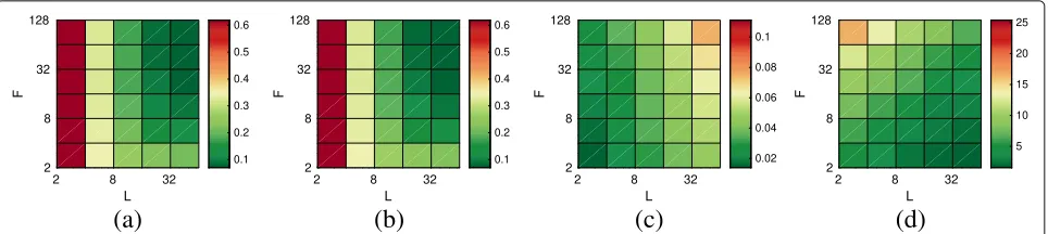
Fig. 2Influence of the parameters (window sizeLand number of graph filtersF) on theaestimation error,bbias,cnormalized standard deviation, anddexecution time. For improved visibility, the scale ofchas been changed
where H = h(G,), H¨ = ¨h(G,), and E[˜ ·] is the
empirical expectation computed over 20 independent experiments. We remind the reader that there are two parameters influencing the performance of the convolutional JPSD estimator (see “Appendix:
Implementation details of the JPSD estimator”: the window size L corresponding to our assumption for the support length of the autocorrelation in time, and the number of graph filters F used to capture power density in the graph spectral dimension. As discussed in Theorem3, the bias will be small as long as the JPSD is a smooth function (it has a small Lipschitz constant), in which case one may opt for smallL andF. Figure2a–d report four key metrics for an exhaustive search ofL,F combinations. We observe that large values of F and L generally reduce the estimation error (Fig. 2a) because they result in reduced bias (Fig.2b). Nevertheless, setting the parameters to their maximum values is not suggested as the variance is increased (Fig.2c).
6.1.3 Complexity
In Fig. 2d, we see that utilizing a large number of fil-ters (i.e., large F) increases the average execution time. Figure3delves further into the issue of scalability. In par-ticular, we vary the number of vertices from 1000 to 9000 and focus on a process with JPSDh(θ)= e−λ/λmaxe−5ω2.
We then examine the min/median/max execution time of the convolutional JPSD estimator for a for increas-ing problem sizes when ran in a desktop computer and repeated 10 times. We compare two implementations. The first, which naively performs the convolution in the spectral domain, uses the eigenvalue decomposition and therefore scales quadratically with the number of vertices. Due to its optimized code and simplicity, this should be the method of choice when N is small. For larger problems, we suggest using the fast implementa-tion. As shown in the figure, this scales linearly with N (here E = O(N)) when the number of filters F and timesteps T are held constant. In this experiment, we setLto 64.
6.1.4 How to choose L and F?
Having no computational constrains, one should choose the parameter combination that minimized the Akaike information criterion (AIC) score AIC = 2FL−2 ln¨, where ¨ is the distribution dependent estimated likeli-hood ¨ = Px| ¨ and ¨ is the estimated covariance based on the convolutional JPSD estimator with param-eters LandF [47]. This procedure is often unfeasible as it is based on computing each model’s log-likelihood and thus entails estimating one JPSD for each parameteriza-tion in consideraparameteriza-tion (as well as knowing the distribuparameteriza-tion
type). We have found experimentally that setting F = min(N, 50) provides a good trade-off between compu-tational complexity and error. On the other hand, we suggest settingLto an upper bound of the autocorrelation support.
6.1.5 Learning from few realizations and a noisy graph
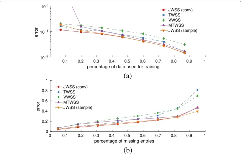
Figure4illustrates the benefit of a joint stationarity prior as compared to (a) an empirical covariance estimator which makes no assumptions about the data and (b) the MTWSS process estimator with optimal bandwidth [22]. As expected, accurate estimation is challenging when the number of realizations is much smaller than the num-ber of problem variables (NT), returning errors above one for the empirical estimator. Introducing stationarity pri-ors regularizes the estimation resulting in more stable estimates.
What is perhaps surprising is that even when the graph (and UG) is known only approximately,
estimat-ing the second order moment of the distribution usestimat-ing the joint stationarity assumption is beneficial. To por-tray this phenomenon, we also plot the estimation error when using a noisy graph (we corrupted the weighted adjacency matrix by Gaussian noise, resulting in an SNR of 10 dB). Undoubtedly, introducing noise to the graph
edges negatively affects estimation by introducing bias. Still, even with noise, the proposed method significantly outperforms purely time-based methods when less than NTrealizations are available.
6.2 Recovery performance on three datasets
We apply our methods on three diverse datasets fea-turing multivariate processes evolving over graphs: (a) a weather dataset depicting the temperature of 32 weather stations over 1 month, (b) a traffic dataset depicting high-resolution daily vehicle flow of 4 weekdays, and (c) SIRS-type epidemics in Europe. Our experiments aim to show that joint stationarity is a useful model, even in datasets which may violate the strict conditions of our definition, and that it can yield a significant improvement in recovery performance, as compared to time- or vertex-based sta-tionarity methods.
6.2.1 Experimental setup
We split theKrealizations of each dataset into atraining setof sizeptKand atest setof size(1−pt)K, respectively.
The training set is used to estimate the JPSD. Then, in the first two experiments, we attempt to recover the values ofpdNT variables randomly discarded from the test set. This corresponds toAbeing a binary diagonal matrix and
(a)
(b)
Fig. 4Estimation errorE˜H¨−HF/HFas a function of the number of realizations and number of vertices. Even an approximate knowledge of the graph enables us to make good estimates of the covariance (and PSD) from few realizations. The joint stationarity prior becomes especially meaningful when the number of variables (N,T) increases. The benefit also holds for a noisy graph (SNR = 10dB).aN=10,T=10
(a)
(b)
Fig. 5Experiments with weather data. The joint approach becomes especially meaningful when the available data are few.aInfluence of the training set size(pd=30%).bInfluence of the percentage of missing values(pt=20%)
w= 0 in ProblemP0, for which the solution is not given by a Wiener filter. In the third experiment, we instead con-sider a denoising problem withA=Iandwbeing a ran-dom Gaussian vector. In each case, we report the RMSE for the recovered signal normalized by the2-norm of the original signal. We compare our joint method with the sample and convolutional JPSD estimators to univariate time/vertex stationarity [17]. These methods solve the statistical recovery problem under the assumption that signals are stationary in the time/vertex domains, but considering different vertices/timesteps as independent. These methods are known to outperform non-model based methods, such as Tikhonov regularization (ridge regression) and total-variation regularization (lasso) over the time or graph dimensions [12,13]. We also compare to the more involvedMTWSS model[25] where the values at different vertices are correlated and the covariance is block circulant of sizeNT×NT(see Definition2). The lat-ter is only shown for the weather dataset as the large num-ber of variables present in the other datasets (e.g.,≈ 108 parameters for the traffic dataset) prohibited computa-tion. We remark that the graph Laplacians we considered did not possess eigenvalue multiplicities, meaning that the results obtained using the JWSS-alternate definition
are identical to that with JWSS using a sample JPSD estimator—thus, we do not include JWSS-alternate in our comparison.
6.2.2 Molene dataset
The French national meteorological service has pub-lished in open access a dataset9 with hourly weather observations collected during the month of January 2014 in the region of Brest (France) [18]. The graph was built from the coordinates of the weather stations by connecting all the neighbors in a given radius with a weight function WG[i1,i2]= exp
−k d(i1,i2)2
, where d(i1,i2) is the Euclidean distance between the stations i1 and i2. Parameter k was adjusted to obtain an aver-age degree around 5 (k however is not a sensitive parameter). We split the data in K = 15 consecutive periods of T = 48 h each. As sole pre-processing, we removed the mean (over time and stations) of the temperature10.
9Access to the raw data is possible directly fromhttps://donneespubliques. meteofrance.fr/donnees_libres/Hackathon/RADOMEH.tar.gz
(a)
(b)
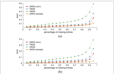
Fig. 6Experiments on Sacramento highway flow. By exploiting both graph and temporal dimensions, the joint approach closely captures the subtle variations in traffic throughout each weekday.a1 out of 4 days used for training(pt=25%).b3 out of 4 days used for training(pt=75%)
We first test the influence of training set sizept, while
discarding pd = 30% of the test variables. As seen in
Fig.5a, due to its large sample complexity, the MTWSS approach provides good recovery estimates when the number of realizations is large, approaching that of joint stationarity, but suffers for small training sets (though not shown in the figure, the relative mean error was 9.8 when onlypt = 10% of the data was used for training).
Due to their stricter modeling assumptions, univariate stationarity methods returned relevant estimates when trained from few realizations but exhibited larger bias. The convolutional JPSD estimator can be seen to improve upon the sample estimator when the amount of data used for JPSD estimation is small (less than 20%). For bigger training sets, the two estimators yield similar accuracy. Figure5b reports the achieved errors for recovery prob-lems with progressively larger percentage 5%≤pd ≤95%
of discarded entries for a training percentage ofpt=20%.
We can observe that the error trends are consistent across all cases.
6.2.3 Traffic dataset
The California department of transportation publishes high-resolution traffic flow measurements (number of
vehicles per unit interval) from stations deployed in the highways of Sacramento11. We focused on 727 stations over four weekdays in the period 01–06 April 2016. Starting from the road connectivity network obtained by the OpenStreetMap.org, we constructed one time series for each highway segment by setting the flow over it to be a weighted average of all nearby stations, while abiding to traffic direction. This resulted in a graph ofN = 710 vertices and a total ofT =24×12 measurements per day forK = 4 days. We used the convolutional JPSD estima-tor with parametersL = T/2 andF = 75, which were experimentally found to give good performance in the training set.
Figure6a and b depict the mean recovery errors when the training sets were 1 (pt =25%) and 3 days (pt=75%)
respectively. The strong temporal correlations present in highway traffic were useful in recovering missing values. Considering both the temporal and spatial dimensions of the problem resulted in accurate estimates, with less than 0.04 error whenpd =50% of the data were removed
and the PSD was estimated from 1 day. As expected, the
(a)
(b)
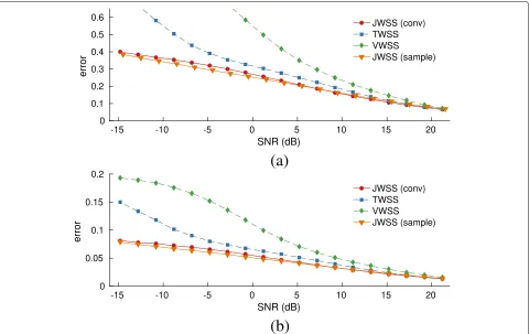
Fig. 7Experiments with the SIRS epidemic model.aInfluence of noise level(pt=50%).bInfluence of noise level(pt=90%)
convolutional estimator is efficient in the case when the training set is small (1 out of 4 days used for training): assuming that the JPSD is smooth helps to reduce estima-tion variance and computaestima-tional complexity but can lead to a slight decrease in accuracy when a large amount of training data is available.
6.2.4 SIRS epidemic
Our third experiment simulates the spread of an infectious disease overN=200 major cities of Europe, as predicted by the susceptible-infected-recovered-susceptible (SIRS) model, one of the standard models used to study epi-demics. We intend to examine the predictive power of the considered methods when dealing with different realiza-tions of a non-linear and probabilistic process over a graph (the data are fictitious). We parameterized SIRS as follows: length of infection period, 2 days; length of immunity period, 10 days; probability of contagion across neighbor-ing cities per day, 0.005; and total period,T = 180 days. We generated a total ofK =10 infections, all having the same starting point.
In contrast to the previous experiments, here, we attempt to recover the data after they have been corrupted with additive Gaussian noise. Figure7a and b depict the mean recovery error as a function of the input
signal-to-noise ratio (SNR), respectively, whenpt =50% andpt =
90% of the data were used for training. As in previous experiments, the joint stationarity attains better recovery. The difference becomes clearer for low SNR, in which case the error is decreased (roughly) by a factor of two w.r.t. the best alternative.
6.2.5 Code
We remark that our simulations were done using the GSP-BOX [48], the UNLocBoX [49], and the LTFAT [50]. The code reproducing our experiments is available athttps:// lts2.epfl.ch/stationary-time-vertex-signal-processing/.
7 Conclusion
This paper proposed a new definition of wide-sense sta-tionarity appropriate for multivariate processes supported on the vertices of a graph.
can be solved in the same asymptotic complexity.Second, joint stationarity is a volatile model, which is able to capture non-trivial statistical relations in the temporal and vertex domains. Our experiments suggested that we can model real spatiotemporal processes as jointly stationary without significant loss. Specifically, the JWSS prior was found more expressive than (univariate) TWSS and VWSS priors and improved upon the multivariate time stationarity prior when the dimensionality was large, but the model estimation was based on few observations of the process.
Appendix
Implementation details of the JPSD estimator
A straightforward implementation requiresON3 oper-ations for computing the eigenbasis of our graph, ON2×KT for performing KT independent GFT, O(Tlog(T) × KN) for KN independent FFT, and ON2T2for the convolution.
This section describes how to approximate a convolu-tional estimate using a number of operations that is linear toET. Before describing the exact algorithm, we note two helpful properties of the estimator. First, we can compute
¨
h(θ)by obtaining estimates for eachX(k) independently
and then averaging overk:
˙
As we will see in the following, the terms inside the outer sum can be approximated efficiently, avoiding the need for an expensive JFT. In addition, when the convolution win-dow is separable, i.e.,g(θ)=gG(λ)·gT(ω), as is assumed in
this contribution, the joint convolution can be performed successively (and at any order) in the time and vertex domains we treat the implementation of the two convolutions sep-arately and the presented algorithms can be combined in any order.
Fast time convolution. This is the textbook case of TPSD estimation that is solved by the Welch’s method [41]. The method entails splitting each time series into equally sized overlapping segments and averaging over segments the squared amplitude of the Fourier coefficients. The pro-cedure is equivalent to an averaging (over time) of the squared coefficients of a short-time Fourier transform (STFT), with half-overlapping windowswT defined such
that DFTwT(t) = gT(ω) [51, 52]. Let L be the
sup-port of the autocorrelation or equivalently the number
of frequency bands. We suggest using the iterated sine window
wT(t)
sin0.5πcos(πt/L)2 ift∈[−L/2,L/2]
0 otherwise,
as it turns the STFT into a tight operator. In order to get an estimate ofh¨ at unknown frequencies, we interpolate between theLknown points using splines [53].
Fast graph convolution. Inspired by the technique of [17], we perform the graph convolution using an approxi-mated graph filtering operation [54] that scales linearly to the number of graph edgesE. In particular,
N
We suggest using the Gaussian window
gG(λ−λn)e−(λ−λn)
2/σ2
, (14)
withσ2 = 2(F+1)λmax/F2. As we did before, we only compute the above forF=O(1)different values ofλand approximate the rest using splines. As the eigenvalues are not known, we need a stable way to estimatecgG(λ). We obtain an unbiased estimate by filteringQ=O(1)random Gaussian signals on the graph ∈ RN ∼ N(0,IN), such
analysis, as it is similar to that in Theorem 2. Accord-ing to our numerical evaluation, the approximation error introduced by the latter estimator and spectral filtering is almost negligible for smooth JPSD.
Univariate vs multivariate JPSD
As discussed in Section 3.2, one could potentially pose a VWSS hypothesis on a product graph to define joint stationarity, but the direct effect of such a choice is that the spectral domain becomes 1-dimensional instead of 2-dimensional. To see why this is problematic, in Fig. 8, we plot the two different representations of the JPSD for the three datasets featured in our experiments. It can be seen that the 2D representation (corresponding to the JWSS hypothesis) is more structured than its 1D coun-terpart. More importantly, a JWSS hypothesis leads to a smoother JPSD: this is what our convolutional JPSD estimator employs to decrease the estimation variance.
Deferred proofs
Proof of Proposition 1In order to simplify the nota-tion in the next proof, we define the unravel funcnota-tion ur : Z2 → Zthat transforms the double indexesn,τ of
the matrix indexing ofXinto its vector index ofu(n,τ)= (τ−1)N+n, i.e.,X[n,τ]=vec(X)[u(n,τ)].
By construction of the JFT basis, X[ 0, 0] captures theˆ DC-offset of a signal, and condition (a) is equivalent to stating that E[x]= c1NT. Moreover, if the graph is
con-nected and (a) holds, at least one of E
Therefore, condition (b) is equivalent to stating that
= UJDU∗J for some diagonal matrixD. In addition,
(c) asserts that D[u(n,τ),u(n,τ)]= h(λn,ωτ) for every
n,τ. Thus, taken together, (b) and (c) state that = UJDU∗J = UJh(G,T)U∗J = h(LG,LT), which is the
second moment condition of a JWSS process.
Proof of Theorem1 For the first moment, it is straight-forward to see that E[X[n,t]] = c if and only if both E[X[n,t]]=ctandE[X[n,t]]=cn∀n,t.
For the second moment, the covariance matrix of a JWSS process is by definition the linear operator associated to a joint filter = h(LG,LT). Using (5), t1,t2 can be
Hence, the process satisfies the (b) statement of Definition2(TWSS) and3(VWSS). Conversely, if a pro-cess is TWSS and VWSS, we have t1,t2 = γt1,t2(LG) =
and hence also satisfies the property of the second moment of JWSS processes.
Proof of Property 2The output of a filter f(LJ) can be
written in vector form asy = f(LJ). If the input signalx
is JWSS, we can confirm that the first moment of the fil-ter output isEf(LJ)x
= f(LJ)E[x]= f(0, 0)E[x], which
remains constant asE[x] is constant by hypothesis. The computation of the second moment gives
y=E
which satisfies the second moment condition of JWSS processes. Above,f2()is a diagonalNT ×NT matrix, whose diagonal is obtained by applying the bivariate func-tionf2(·,·)on [λn,ωτ] for alln,τ(f can be interpreted as
the frequency response of a joint filter). MatrixhX()is
similarly defined.
Lemma 2 IfXis a JWSS process such that the entries ofXˆ are independent random variables, the convolutional JPSD estimate atθ has variance
Var
is the variance of the sample JPSD estimator atθn,τ.
ProofSet
αn,τ =g(θ−θn,τ)2h(θn,τ)/cg(θ)
andEˆ(k)= matˆ(k)=mat(h(G,)+1/2xˆ(k)), where+
denotes the pseudo-inverse,ˆ(k)is white, and mat(·)is the
matricization operator. The centered random variable
¨
is a weighted sum of centered, identically distributed ran-dom variableszn,τ. Moreover, when the elements ofEˆ
¯(k) are independent, so are the variableszn,τ. It follows that
Var
AIC: Akaike information criterion; DFT: Discrete Fourier transform; GFT: Graph Fourier transform; JFT: Joint Fourier transform; JPSD: Joint power spectral density; JWSS: Jointly wide-sense stationary; MTWSS: Multivariate time wide-sense stationary; MVWSS: Multivariate vertex wide-sense stationary; PSD: Power spectral density; TPSD: Time power spectral density; TWSS: Time wide-sense stationarity; VPSD: Vertex power spectral density; VWSS: Vertex wide-sense stationarity; WSS: Wide-sense stationarity
Acknowledgements
We thank Francesco Grassi for his help with the code.
Authors’ contributions
The two authors contributed equally both for the experiments and for the writing of the paper. Both authors read and approved the final manuscript.
Funding
This work has been supported by the Swiss National Science Foundation research projectTowards Signal Processing on Graphs(grant number: 2000_21/154350/1) and research projectDeep Learning for Graph-Structured Data(grant number: PZ00P2 179981).
Availability of data and materials
The code to reproduce the results is available at https://lts2.epfl.ch/stationary-time-vertex-signal-processing/.
• Access to the raw Molene dataset is possible directly fromhttps:// donneespubliques.meteofrance.fr/donnees_libres/Hackathon/ RADOMEH.tar.gz
• The traffic data corresponding to the 3rd district of California and can be downloaded fromhttp://pems.dot.ca.gov/.
• The epidemic dataset is synthetically generated from a SIR model. The network used for the model can be downloaded fromhttps://www. visualizing.org/global-flights-network/.
Competing interests
The authors declare that they have no competing interests.
Author details
1Laboratoire de Traitement des Signaux 2, École Polytechnique Fédérale
Lausanne, 1015 Lausanne, Switzerland.2Swiss Data Science Center, Eidgenössische Technische Hochschule Zürich, Universitätstrasse 25, 8006 Zürich, Switzerland.
Received: 29 November 2018 Accepted: 2 July 2019
References
1. M. Rudelson, Random vectors in the isotropic position. J. Funct. Anal. 164(1), 60–72 (1999)
2. H. Lütkepohl, New introduction to multiple time series analysis. Springer Sci. Bus. Media (2005)
3. O. Ledoit, M. Wolf, A well-conditioned estimator for large-dimensional covariance matrices. J. Multivar. Anal.88(2), 365–411 (2004)
4. C. Lam, Q. Yao, et al., Factor modeling for high-dimensional time series: inference for the number of factors. Ann. Stat.40(2), 694–726 (2012) 5. G. Connor, The three types of factor models: a comparison of their
explanatory power. Financ. Anal. J.51(3), 42–46 (1995)
6. M. J. Keeling, K. T. Eames, Networks and epidemic models. J. R. Soc. Interface.2(4), 295–307 (2005)
7. P. Mohan, V. N. Padmanabhan, R. Ramjee, inProceedings of the 6th ACM Conference on Embedded Network Sensor Systems. Nericell: rich monitoring of road and traffic conditions using mobile smartphones (ACM, 2008), pp. 323–336
8. W. Huang, L. Goldsberry, N. F. Wymbs, S. T. Grafton, D. S. Bassett, A. Ribeiro, Graph frequency analysis of brain signals. IEEE J. Sel. Top. Signal Proc. 10(7), 1189–1203 (2016)
9. F. Zhang, E. R. Hancock, Graph spectral image smoothing using the heat kernel. Pattern Recog.41(11), 3328–3342 (2008)
10. A. J. Smola, R. Kondor, Kernels and regularization on graphs. Learning theory and kernel machines, 144–158 (2003)
11. M. Belkin, P. Niyogi, Semi-supervised learning on riemannian manifolds. Mach. Learn.56(1–3), 209–239 (2004)
12. D. I. Shuman, S. K. Narang, P. Frossard, A. Ortega, P. Vandergheynst, The emerging field of signal processing on graphs: Extending
high-dimensional data analysis to networks and other irregular domains. Signal Process. Mag. IEEE.30(3), 83–98 (2013)
13. A. Sandryhaila, J. M. Moura, Discrete signal processing on graphs. IEEE Trans. Signal Process.61, 1644–1656 (2013)
14. A. Sandryhaila, J. M. Moura, Big data analysis with signal processing on graphs: Representation and processing of massive data sets with irregular structure. IEEE Signal Process. Mag.31(5), 80–90 (2014)
15. A. Gadde, A. Ortega, inInternational Conference on Acoustics, Speech and Signal Processing (ICASSP). A probabilistic interpretation of sampling theory of graph signals (IEEE, 2015), pp. 3257–3261
16. C. Zhang, D. Florêncio, P. A. Chou, Graph signal processing–a probabilistic framework. Microsoft Res. (2015). Redmond, WA, USA, Tech. Rep. MSR-TR-2015-31
17. N. Perraudin, P. Vandergheynst, Stationary signal processing on graphs. IEEE Trans. Signal Process.65(13), 3462–3477 (2017).https://doi.org/10. 1109/TSP.2017.2690388
18. B. Girault, inSignal Processing Conference (EUSIPCO), 2015 23rd European. Stationary graph signals using an isometric graph translation (IEEE, 2015), pp. 1516–1520