Gaussian Channel Model for Mobile Multipath Environment

(1)

Gaussian Channel Model for Mobile

Multipath Environment

D. D. N. Bevan

Harlow Laboratories, Nortel Networks, Harlow, Essex CM17 9NA, UK Email:[email protected]

V. T. Ermolayev

Communication Systems Research Department, MERA Networks, Nizhny Novgorod 603126, Russia Email:[email protected]

A. G. Flaksman

I. M. Averin

Received 28 May 2003; Revised 5 February 2004

A model of an angle-spread source is described, termed the “Gaussian channel model” (GCM). This model is used to represent signals transmitted between a user equipment and a cellular base station. It assumes a Gaussian law of the scatterer occurrence probability, depending upon the scatterer distance from the user. The probability density function of the angle of arrival (AoA) of the multipath components is derived for an arbitrary angle spread. The “wandering” of the “centre of gravity” of the scattering source realisation is investigated, which is in turn due to the nonergodicity of the angle-scatter process. Numerical results obtained with the help of the sum-diﬀerence bearing method show the dependence of the AoA estimation accuracy on the spread-source model.

Keywords and phrases:scattering, angle spread, channel model, angle-of-arrival estimation, multibeam.

1. INTRODUCTION

The implementation of smart antennas at macrocellular base stations (BSs) is expected significantly to enhance the capac-ity of wireless networks [1,2]. Various algorithms for adap-tive array signal processing have been proposed and investi-gated [2,3,4]. The eﬀectiveness of these algorithms depends on the behaviour of the fading channel and in particular on the degree of azimuthal dispersion in the channel. Therefore, accurate statistical channel models are required for the test-ing of these adaptive algorithms. These models must be re-alistic and close to real-life channels in order to replicate the angle of arrival (AoA) distribution of the multipath compo-nents.

The propagation channel between the BS and the user equipment (UE) is generally held to be reciprocal in most respects. However, the azimuthal angle dispersions seen at

(2)

radius and upon the distance between BS and user. However, in a real-life channel, the scatterer distribution around the UE can diﬀer significantly from uniform. Therefore, other researchers [9, 10,11] have proposed other more realistic models based on a Gaussian distribution of scatterer loca-tion.

The goal of this paper is to analyse further the Gaussian proposal for the scatterer distribution. We assume that the scatterers can be situated inanypoint in the horizontal plane. In this model, the probability of occurrence of the scatterer location decreases in accordance with a Gaussian law when its distance from the UE antenna increases. Therefore, we call this model the “Gaussian channel model (GCM).” We believe that such an assumption about the scatterer location is closer to the real-life environment than some of the other models mentioned above. Therefore, as we will demonstrate later, the comparison of the obtained pdf of AoA of the multipath for the GCM with the measured results presented in [8] gives very good agreement. Note also that, like Clarke’s model, the proposed GCM also provides the classical Doppler sig-nal spectrum.

It is a likely supplementary requirement for future cellu-lar communication systems that they will be capable of de-termining the user position within a cell site. One way of do-ing this is via “triangulation,” whereby the angular beardo-ing of the user is estimated at multiple cellsites (this process is also known as “direction finding”). UE position is estimated as the point where these bearing lines intersect. Thus, in or-der to carry out triangulation, an estimate of the AoA of the UE signal is required. We consider the “sum-diﬀerence bear-ing method” (SDBM) algorithm for AoA estimation. It was selected from a number of techniques that had been investi-gated (see, e.g., [12,13,14]). The SDBM algorithm is similar to the principle used in monopulse tracking radars, wherein a hybrid junction is used to extract the sum and diﬀerence of a received pulse [12]. Note that the tracking radar is able to serve just one user. However, the multibeam antenna ar-rays at the BS can serve all the users located in the given cell. More details of this SDBM algorithm will be provided later.

One of the major aims of the BS is to achieve a high capacity. To maximise the downlink capacity, it has been proposed elsewhere to use multibeam or beamformed an-tenna arrays to cover each sector of the cell handled by the BS [15]. Such an antenna array could also be ap-plied to estimate the AoA. Therefore, in this paper, the de-pendence of the AoA estimation accuracy on the spread source model is also considered for the BS using a multi-beam antenna. In this configuration, the multi-beamformer cre-ates three fixed beams per 120◦-azimuth sector, generated from a facet containing 6-oﬀλ/2-spaced columns of dual-polar antenna elements. These beams improve the cover-age and capacity of the macrocell, and are expected to have greatest application within the urban macrocellular en-vironment, where the need for maximum capacity is the greatest. Simulation results are presented for the case of a Rayleigh fading channel and for this antenna configura-tion.

y(y) UE reﬀ

x

θeﬀ

D

R θ

BS x

Figure1: Illustration of the Gaussian channel model.

2. GAUSSIAN CHANNEL MODEL AND THE PDF OF

THE AOAS OF MULTIPATH COMPONENTS SEEN AT THE BASE STATION

The signal received by the BS is a sum of many signals re-flected from diﬀerent scatterers randomly situated around the UE antenna. The AoAs of the multipath signal compo-nents are thus various and random. Therefore, the set of the scatterers can be considered collectively as a spread source, and the angle spread is a measure used to determine the an-gular dispersion of the channel.

Here we present the details of the GCM and derive an analytical expression for the pdf of the AoAs of multipath components as observed at the BS.

First of all, we list the initial assumptions used for creat-ing the channel model. We assume that

(i) the scattered signals arrive at BS in the horizontal plane, that is, the proposed GCM is two dimensional and the elevation angle is not taken into account; (ii) each scatterer is an omnidirectional reradiating

ele-ment and the plane wave is reflected directly to the BS without influence from other scatterers (i.e., we have only “single-bounce” scattering paths);

(iii) the direct path from the UE to BS antenna is infinitely attenuated;

(iv) the reflection coeﬃcient from each scatterer has unity amplitude and random phase;

(v) the probability of the (random) scatterer location is in-dependent of azimuth angle (from the UE), and de-creases if its distance from the UE antenna inde-creases. This dependence has a Gaussian form.

The last of these assumptions distinguishes our channel model from many of the other known models [5,6,7].

Thus we can write that

p(r,ϕ)= 1

πre2ﬀ exp

− r2

re2ﬀ

, (1)

where (r,ϕ) is the polar coordinate system centred at the UE,

ris the distance to a given scatterer from the UE antenna, and

(3)

whereDis the distance between the BS and UE antennas, and (x,y) are the rectangular coordinates.

In [7], a uniform scatterer distribution within the cir-cle of radius r0 around the UE was assumed. So for the model of [7], this means that the AoAs of multipath com-ponents seen at the BS are limited to the angular region [−θmax· · ·θmax], whereθmax = sin−1(r0/D). However, for our GCM model, the AoAs of scattered signals as received at the BS are not restricted to any constrained angular re-gion.

In order to derive the ensemble pdf of the AoA for the GCM (i.e., averaged over many model realisations), we choose the origin of the system coordinates (x,y) to be the location of the BS. This means thatx=xandy = y+D. We then transform to the polar coordinates (R,θ), where

x=Rsinθ,y=Rcosθ, and the angleθis measured rela-tive to the line joining the BS and UE antennas. It is straight-forward to show that the Jacobian of this transformation is equal toR. Furthermore, we have

r2₌_x2₊_y2₌_x2₊_y₋_D2

In order to derive the one-dimensional pdf of the AoA (i.e., the power angle density) of the multipath components as seen at the BS, an integration over the radiusRmust be carried out. Therefore, the pdf is expressed as the following integral:

This integral can be calculated analytically and a closed-form solution is obtained. To do this, take into account that (see [16, equation 3.462.1])

_∞

is the function of the parabolic cylinder. In our case, we have

v =2,β = r−2

eﬀ, andγ = −2Dre−ﬀ2cosθ. Ifv =2, then the functionC−2(z) can be expressed in terms of the probability

integralΦ(z) (see [16, equation 9.254.2]1_{), that is,} straightforward transformations, we can obtain from (5) and (6) that the desired one-dimensional pdfp(θ) of AoA of the multipath components is given by

p(θ)= 1

The expression (8) is true in the general case. However, this formula takes a very simple form for the case of small angle spreadθeﬀ πwhen sinθ≈θ. In this case, the pdf is

and described by a (one-dimensional) Gaussian pdf with zero mean and varianceσ2₌₀_.₅_θ2

eﬀ.

Figure 2 shows the pdf p(θ) of the AoA of the

multi-path components for the different valuesθeff =10◦, 30◦, and 50◦. The solid and dashed curves correspond to the exact formula (8) and to its Gaussian approximation (9), respec-tively. We can see that the exact and Gaussian PDFs are very close to each other for a large interval ofθeff up toθeff ≤0.5 (orθeff ≤ 30◦). Actually, it is quite simple and intuitive to see how the complex pdf of the exact formula (8) should

1_{N.B. There is a minor typographical error (a missing factor of}₋_{1) in}

(4)

75

Figure2: The pdf of the AoA of the multipaths at the BS. The angle spread is equal to 20, 60, and 100 degrees (curves 1, 2, 3, respec-tively). The solid and dashed curves correspond to the exact formula (8) and its Gaussian approximation (9), respectively.

equal a one-dimensional pdf for small angle spreads. At these small angles, the lines bounding diﬀerent small “slices” of the two-dimensional pdf are nearly parallel, and so it is as if we are calculating the marginal pdf of the two-dimensional spatial pdf along the x-axis. Since the marginal pdf of a two-dimensional Gaussian distribution is a one-dimensional Gaussian distribution, our approximate result (9) is intu-itively of the correct form.

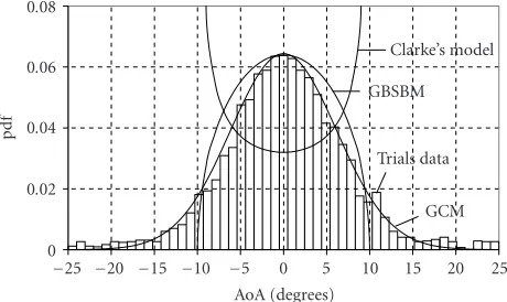
The comparison of the theoretical pdf against real mea-surement data is of course of interest in order both to val-idate and to parameterise the GCM. Histograms of the es-timated azimuthal power angle density and scatterer occur-rence probabilities are presented by the authors of [8]. This measurement data was obtained in Aarhus with a BS antenna located 12 m above the rooftop level. We wish to take this measured data and compare it to the three proposed theoreti-cal channel models: (1) our GCM of (8), (2) the geometrical-based single-bounce model (GBSBM) developed in [7] (in which the scatterers are assumed to be uniformly randomly distributed within the area of a circle), and (3) Clarke’s model [5,17] (in which the scatterers are assumed to lie on the cir-cumference of a circle).

It was derived in [7] that the pdf of the AOA of the mul-tipath components for GBSBM is given by

p(θ)= within which all the scatterers are uniformly distributed.

Whilst we omit the derivation here, for reasons of brevity, it can be shown that the pdf of the AOA of the multipath components for Clarke’s model is equal to

p(θ)= 1

where in this case, when calculatingθmax,r0has the meaning

25

Figure3: The PDFs for the AoA of the multipath components at the BS for GCM, GBSBM, Clarke’s models, and for the measured histograms.

of the radius of the circle periphery on which the scatterers are uniformly distributed.

Figure 3shows the PDFs for the AoA of the multipath

components at the BS for GCM, GBSBM, Clarke’s mod-els, and the measured scatterer occurrence probability his-tograms taken from [8]. We have chosen the model param-eters (θmax,θeﬀ) so that the best agreement was obtained for

each model. For both the GBSBM and Clarke’s models, the value chosen wasθmax = 10◦, and for GCM,θeﬀ =8.8◦. It can be seen that the GCM ensures the best agreement with real-life results for the whole angular region and especially for the tails of histogram. Clarke’s model produces the worst match to the real-life data.

The measured data and experimental models described above discuss the “ensemble” statistics of the spread source. By ensemble statistics, we mean that these statistics are aver-aged over a large number of individual measurements or in-dividual model realisations. However, in practice, we would deal with single cases (i.e., in “real-life”) or single-model re-alisations (i.e., during simulation). It seems reasonable to postulate that the angle-spread behaviour of the source will be nonergodic. That is to say, the statistics of any given re-alisation (averaged over time) will, in general, be diﬀerent from the ensemble statistics (averaged over all realisations andalltime). So in practice, in any single realisation of the angle-spread model, we will see a limited number ofdiscrete

(5)

apparent change of the UE bearing for diﬀerent realisations of the scattering model, which we term the “wandering” of the “CofG” is a direct consequence of the nonergodicity of the angle-scattering model. This wandering is more marked when the mean number of scattering sources is low, because if we have a large number of scattering sources, then it would beextremelyunlikely forallof them to be lying on the same side of the UE (assuming that all scatterer locations are in-dependent). In fact, we will show later that this “wandering of the CofG” phenomenon is a significant contributor to the overall estimation error of the UE bearing.

For reasons described above, the variance of the wander-ing of the CofG depends on the number of scatterers situated around the UE antenna. LetN be the number of scatterers andθ1,θ2,. . .,θNsome random values of AoAs of the signal

from these scatterers. Assume, for simplicity, that all of the sources have equal power. Then the CofG of the received sig-nal for this particular realisation is equal to

The expectation of the random valueθis equal to zero (i.e.,θ =0) and its variance can be obtained from the

in-pendent random values, the joint pdf can be presented as the product of individual PDFs, that is, p(θ1,θ2,. . .,θN) =

p(θ1)p(θ2)· · ·p(θN), where the function p(θi) (i =

1, 2,. . .,N) is given by formula (8).

Theexpectedazimuth angle of each angle-spread source is equal to zero due to the symmetry of the pdf (8) of the multipath component AoAs, that is,θi =0. Thus theN

-dimensional integral (13) can be rewritten as the sum ofN

identical one-dimensional integrals, that is,

σ2

1θis the variance of the AoA of a single scatterer, equal

to wandering of the CofG of the spread source when we assume

Nscatterers of the same amplitude.

For smallθeﬀ 1, the pdf p(θ) has Gaussian form (9). Substituting (9) into (15) and carrying out the integration

120

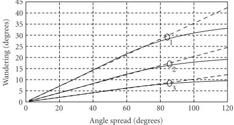
Figure4: The source C of G wandering versus angle spread∆for the diﬀerent numbers of scatterersN =1, 3, 12 (curves 1, 2, 3, re-spectively). The solid and dashed curves correspond to the exact formula (8) and its Gaussian approximation (9), respectively.

in (15), we obtain thatσ1θ=θeﬀ/√2. Hence it can be found

from (14) that the wandering of the CofG is equal to

σNθ =√θeﬀ

2N. (16)

Figure 4 shows the wanderingσNθ of the CofG of the

source versus angle spread∆for diﬀerent numbers of scatter-ersN=1, 3, 12 (curves 1, 2, 3). The solid and dashed curves correspond to the exact formula (8) and its Gaussian approx-imation (9), respectively. We can see that the exact and Gaus-sian PDFs are very close to each other for a large interval of

θeﬀup to≈40◦.

The CofG of the scattering sources gives the best unbi-ased estimate of the true UE bearing, albeit that it is an esti-mate with high variance (i.e., high mean squared error) when the number of scattering centres is small. So the aim of our AoA estimation processing is to estimate this CofG from a limited-time snapshot of noisy received signal. The receiver noise will add an additional error term to the final bearing estimation error. However, it can be seen from the forego-ing analysis that even usforego-ing “perfect” CofG estimation algo-rithms on long samples of high signal-to-noise-ratio (SNR) received signal, there will still be a residual irreducible error if the number of scattering centres is small. This is because of the wandering of the CofG, which in turn is due to the nonergodicity of the spread source.

3. AOA ESTIMATION INCORPORATING THE GCM

(6)

the less-than-perfect algorithm (compared to an optimal al-gorithm) are small compared to the irreducible CofG wan-dering error which we must allow for in any case. So in this section, we consider just such a simplified AoA estimation process, which we term SDBM. This method was selected from a number of similar techniques which had been inves-tigated because it was found to give the overall most accurate and most robust performance. The mathematical details of the SDBM technique will be presented later. However, the essence of the technique is to measure, average, and com-pare received signal powers (or amplitudes) received at the BS, as measured in adjacent beams. We assume, for the use of SDBM, that the BS already employs a multibeam antenna (typically with three deep-cusp beams) in each 120◦-azimuth sector. The scattered signal from the user is received by each of the beams of the antenna, and the two adjacent beams receiving the highest signal powers are selected. For these beams, a set of functions, which we term “bearing curves,” must be precalculated and stored. The exact form of these bearing curves depends upon the multibeam antenna pat-terns and upon the expected ensemble angle-spread distri-bution (which we argued earlier tends to Gaussian form at small angle spreads).

First of all, we determine the dependence of the average received powerGat an arbitrary beam output on the angle location of the source with an angle spread∆. LetF(θ) be the reception gain pattern of this beam andθ0be the centre of the spread source (i.e., the “true” UE bearing). Then the function

G(θ0) can be presented in form of a mathematical convolu-tion of (i) a funcconvolu-tion representing the power beam pattern |F(θ0)|2_{of this beam as a function of the azimuth angle (}_θ₎ and (ii) a function p(θ) representing the (ensemble) pdf of the AoAs of signals received by the BS due to reflections from scatterers as a function of azimuth angle (θ), that is,

Gθ0

= _π

0

_F(θ)2pθ−θ0

dθ. (17)

We can refer to the function (17) as a “beam pattern for a spread source,” that is, what we call a “spread” beam pat-tern. If the spread of signals is a negligibly small quantity (θeﬀ →0), then we have a point source, and the pdfp(θ) in

(8) tends to a delta function (i.e., p(θ)→δ(θ−θ0)). In this case, the functionG(θ0) is given byG(θ0)= |F(θ0)|2_{, that is,} it is simply equal to the power gain pattern of the beam, or to what we will term the “point source” beam pattern.

Now we provide the mathematical definition of what we have termed earlier the “bearing curves.” IfLis the number of the beams generated by the multibeam antenna, then we have a set of beam patternsGi(θ) (i=1, 2,. . .,L) and each beam

pattern is oriented in a given direction. The bearing curves

bi+1,i(i = 1, 2,. . .,L−1) for each adjacent beam pair (i+

1,i) may be represented by a functionbi+1,i(θ) of the azimuth

angleθof the antenna according to the following equation:

bi+1,i(θ)=

Gi(θ)−

Gi+1(θ)

Gi(θ) +

Gi+1(θ).

(18)

Measure mean power over some observation

interval p3

p2

p1

3 2 1

Deep-cusp

beamfor

m

er

3 2

1

Sour ce bear_ing

Figure5: Applying the SDBM algorithm.

These bearing curves are precalculated and stored by the network. The precalculation takes place based on equation (17), and hence takes into account both the known multi-beam patterns and theexpectedangle-spread distribution of the scattering channel (which we model as Gaussian with a givenθeﬀ). There is more discussion later about how we de-termine the expected angle spread.

To estimate the bearing of any given source, the received power from each beam of the antenna is measured over a predetermined observation interval by averaging over a large number of samples. The observation interval should be cho-sen to be long enough so that the eﬀects of Doppler signal fading do not significantly impact the measured power.

The application of SDBM algorithm is shown inFigure 5. Let pi = |si(t) +ni(t)|2be the mean power measured at the

output of theith (i=1, 2,. . .,L) antenna beam, wheresi(t)

andni(t) are the useful signal and additive white Gaussian

noise (AWGN), respectively. The AWGN varianceσ2 0 is as-sumed to be the same for all of the diﬀerent antenna beams. The bearing curves, per (18), are produced without regard to AWGN. That is to say, they only take into account ratios of sums and diﬀerences of expectedsignalamplitudes (with-out including noise or interference contributions). There-fore, for a more accurate estimation of AoA based on mea-sured noisy samples, we need to take into account anexpected

noise power contribution for the measured signal, the value of which we subtract from themeasuredpower signal of each beam after the averaging. In practice, this means that we use an estimated output signal power equal to pi = |pi−σ02|. The estimates pi for all i = 1, 2,. . .,Lare compared with

each other and the two adjacent beams receiving the high-est signal powers are selected. If the jth and (j+ 1)th beams have the highest output powers, then the sum-diﬀerence ra-tio ˆbj+1,j=(

pj−

pj+1)/(

pj+

pj+1) is calculated and the

AoA is estimated by looking up the bearingθcorresponding to this ratio from the corresponding bearing curvebj+1,j(θ)

of (18).

(7)

60

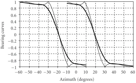
sources (thin and thick curves, respectively).

dual-polar antenna elements (although only a single polari-sation is considered here). The angular spread of the source will be assumed to be equal to 17◦, which corresponds to ex-perimental results obtained in [8]. Two representative cases, for which the number of scatterers is specified asN=3 and

N = 12, will be simulated. There are two bearing curves

b21(θ) andb32(θ) for the antenna configuration with three beams.

The bearing curvesb21(θ) andb32(θ) for the point (∆= 0◦) and spread (∆=17◦) sources are presented inFigure 6

(thin and thick curves, respectively). The left-hand curves are b21(θ) and the right-hand curves are b32(θ). It can be seen that these bearing curves have the steepest slope at the points where the beams cross. Estimation of the bearing of the point source is possible only in the angle intervals [−30◦_, −10◦_{] and [10}◦_{, 30}◦_{]. For the spread source, estimation of} the bearing is possible over wider angle intervals [−35◦_{, 35}◦_]. It is assumed, of course, that to estimate the bearing of UEs for angles outside this range, we would construct additional bearing curves relating to the beam at the edge of this sector and its neighbour at the edge of the adjacent sector.

When estimating the AoA, the estimatesp1,p2, andp3of the mean signal power at the output of theith (i = 1, 2, 3) antenna beam are compared with each other. Ifp1>p3, then the ratio ˆb21is calculated and the AoA is estimated using the bearing curveb21(θ). If p1 < p3, then the value ˆb32is calcu-lated and the AoA is estimated according to the bearing curve

b32(θ).

Within the simulations, the samples of the complex sig-nals were generated with a sampling period equal to 1 mil-lisecond for three antenna beams. The maximum Doppler frequency fd was set equal to 50 Hz. The observation

inter-val was chosen to be 400 milliseconds, that is, approximately 50 times longer than the fading correlation interval. Various SNRs equal to 30, 20, 10 and 0 dB were simulated, where the SNR is defined by what the received SNR is for a point source located at the peak of the central beam. In order to average the results over all source directions, the true source angle θtrue was varied from −40◦ to +40◦ with a step size equal to 0.5◦. A thousand experiments were carried out for

30

Figure7: The rms of bearing estimation error for various SNRs and for the number of scatterersN=3.

each source direction, and diﬀerent realisations of the (non-ergodic) source model were applied for each of these experi-ments. For each source position, the root-mean-square (rms) ∆θ of the bearing estimation error and the cumulative

den-sity function (CDF) of absolute value of AoA estimation er-ror|_θˆ_j₋_θ_true|_{were calculated.}

The rms of the bearing estimation error is shown in

Figure 7for the number of scatterersN=3 and for the given

SNRs. We can see that, as expected, the rms of the bearing estimation error decreases when the SNR increases. For large SNRs (20 and 30 dB), the bearing estimation error lies within the range 2◦ to 6◦ (depending on the true source bearing) and is solely due to the random wandering of the CofG of the angle-spread source. For the lower SNRs, the bearing estima-tion error is larger, and depends also on AWGN power. The corresponding CDFs are presented inFigure 8. The CDFs in

Figure 8can be approximated by the CDF of a Gaussian

func-tion. Using this Gaussian approximation, we obtain that the standard deviation of the bearing estimation error is≈4◦for high SNRs andN=3. As can be seen fromFigure 4(curves 2), this standard deviation is approximately equal to the stan-dard deviation of the wandering of the CofG of the source with an angle spread∆ = 2θeﬀ = 17◦ (θeﬀ = 8.5◦). Thus we can see that the bearing estimation error for high SNRs is conditioned by the nonergodicity of the source model. The highest bearing estimation errors are observed in the cross-ing area of the antenna beam patterns. This is because the beam gains are lower in this angular region, and so the ef-fective received SNR is also lower in this region compared to what it would be for a source located close to the peak of the central beam. The CDF of the bearing estimation error for a larger number of scatterersN=12 is also shown inFigure 8. Compared to the results forN = 3, the standard deviation of the bearing estimation error has decreased by a factor of approximately two for high SNRs, from≈4◦ to≈2◦. Like the results forN =3, this also corresponds toFigure 4and (14).

(8)

15 10

5 0

Bearing error (degrees) 0

0.25 0.5 0.75 1

CDF

0 dB 10 dB 20, 30 dB

Figure 8: The CDFs of the bearing estimation error for various SNRs. The number of scatterers isN=12 (solid curves) andN=3 (dashed curves).

of the bearing curves involves a convolution of the actual

beam pattern with theassumedangle-spread ensemble pdf. What if we didn’t apply the preconvolution in the genera-tion of the bearing curves, but simply used the bearing curve corresponding to “point source” beam patterns, even when the channel itself doesexhibit angle spread? To answer this, it is interesting to examine the bearing errors when bearing curves generated for the point source are actually used for es-timating AoA in a channelwithangle spreading. Such com-parative simulation results for the CDF of the bearing error are presented inFigure 9for SNR = 30 dB and number of scatterersN =12. The angle spread in the channel is equal to 17◦. We can see that the bearing error has increased sig-nificantly due to the use of “nonmatched” bearing curves. In order to generate “matched” bearing curves, we need at least to have a reasonable estimate of the (ensemble) angle spread of the channel. In practice, this would be obtained through examination of published measured angle-spread data such as [8], and by matching the environment in which the multi-beam BS is deployed (e.g., urban, suburban, rural) to the ex-pected angle spread of the channel.

4. CONCLUSIONS

In this paper, we have developed a model for an angle-spread source which we term the Gaussian channel model (GCM). This model is suitable for representing the signal seen at the base station (BS) antenna, and assumes that the probabil-ity of the scatterer occurrence decreases in accordance with a Gaussian law when its distance from the user equipment (UE) antenna increases. Such an assumption about the scat-terer location is closer to the real-life environment than some of the other known models. An analytical expression for the probability density function (pdf) of the multipath angle of arrival (AoA) at the BS has been derived for the general case of an arbitrary angle spread. It is shown that this pdf can be approximated by a Gaussian curve for sources with a small spread. The comparison of the obtained pdf of AoA of the multipath for the GCM with the published experimental re-sults gives a better agreement than for some other known

8 6

4 2

0

Bearing error (degrees) 0

0.25 0.5 0.75 1

CDF

Figure 9: The CDF of the bearing estimation error using the “spread” bearing curve (thick curve) and “point source” bearing curve (thin curve) for SNR = 30 dB, angle spread∆ =17◦_{, and}

number of scatterersN=12.

angle scattering models. However, in a real-life situation, we deal with a single realisation of the angle-spread source, that is, with a fixed finite number ofdiscretescattering centres. If this number is particularly small, then their center of grav-ity (CofG), defined as a power-weighted average AoA, may “wander” about the true bearing of the UE. The variance of this wandering of the CofG has been obtained. The depen-dence of the AoA estimation accuracy on the parameters of the spread source model has also been considered for a BS us-ing a multibeam antenna, by carryus-ing out simulations of the so-called sum-diﬀerence bearing method (SDBM) AoA esti-mation algorithm. It has been shown that for high SNRs, the bearing estimation errors are dominated by the wandering of the CofG of the spread source. This wandering is a con-sequence of the nonergodicity of the angle scattering process and is greater when the number of scattering sources is small.

REFERENCES

[1] J. C. Liberti and T. S. Rappaport, Smart Antennas for Wireless Communications: IS-95 and Third Generation CDMA Applica-tions, Prentice Hall, Upper Saddle River, NJ, USA, 1999. [2] J. B. Andersen, “Antenna arrays in mobile communications:

gain, diversity, and channel capacity,” IEEE Antennas and Propagation Magazine, vol. 42, no. 2, pp. 12–16, 2000. [3] U. Vornefeld, C. Walke, and B. Walke, “SDMA techniques for

wireless ATM,” IEEE Communications Magazine, vol. 37, no. 11, pp. 52–57, 1999.

[4] R. A. Soni, R. M. Buehrer, and R. D. Benning, “Intelligent an-tenna system for cdma2000,”IEEE Signal Processing Magazine, vol. 19, no. 4, pp. 54–67, 2002.

[5] R. H. Clarke, “A statistical theory of mobile-radio reception,” Bell System Technical Journal, vol. 47, no. 6, pp. 957–1000, 1968.

[6] J. C. Liberti and T. S. Rappaport, “A geometrically based model for line-of-sight multipath radio channels,” inProc. IEEE 46th Vehicular Technology Conference, vol. 2, pp. 844– 848, Atlanta, Ga, USA, April 1996.

[7] P. Petrus, J. H. Reed, and T. S. Rappaport, “Geometrical-based statistical macrocell channel model for mobile environ-ments,”IEEE Trans. Communications, vol. 50, no. 3, pp. 495– 502, 2002.

(9)

the base station in outdoor propagation environments,”IEEE Trans. Vehicular Technology, vol. 49, no. 2, pp. 437–447, 2000. [9] J. Fuhl, A. F. Molisch, and E. Bonek, “Unified channel model for mobile radio systems with smart antennas,” IEE Proceed-ings Radar, Sonar and Navigation, vol. 145, no. 1, pp. 32–41, 1998.

[10] R. M. Buehrer, S. Arunachalam, K. H. Wu, and A. Tonello, “Spatial channel model and measurements for IMT-2000 sys-tems,” inProc. IEEE Vehicular Technology Conference, vol. 1, pp. 342–346, Rhodes, Greece, May 2001.

[11] Lucent Technologies, “Proposal for a spatial channel model in 3GPP RAN1/RAN4,” Contribution WG1#20(01)579 of Lu-cent Technologies to 3GPP-WG1, Busan, May 2001.

[12] M. I. Skolnik, Ed.,Radar Handbook, McGraw-Hill, New York, NY, USA, 1970.

[13] O. Besson, F. Vincent, P. Stoica, and A. B. Gershman, “Ap-proximate maximum likelihood estimators for array process-ing in multiplicative noise environments,”IEEE Trans. Signal Processing, vol. 48, no. 9, pp. 2506–2518, 2000.

[14] S. Valaee, B. Champagne, and P. Kabal, “Parametric localiza-tion of distributed sources,”IEEE Trans. Signal Processing, vol. 43, no. 9, pp. 2144–2153, 1995.

[15] M. S. Smith, M. Newton, and J. E. Dalley, “Multiple beam antenna,” US Patent number 6,480,524, November 2002. [16] I. S. Gradshteyn and I. M. Ryzhik,Table of Integrals Series and

Products, Academic Press, New York, NY, USA, 1965. [17] W. C. Jakes, Ed., Microwave Mobile Communications, John

Wiley & Sons, New York, NY, USA, 1974.

D. D. N. Bevan received his M.Eng. in electronic and electrical engineering from Loughborough University of Technology in 1991. Since then, he has worked in the field of radio technology within the Wire-less Technology Laboratories of Nortel Net-works in Harlow, UK. His research inter-ests include system modelling, array sig-nal processing, and technologies for current and future wide-area and local-area wireless networking.

V. T. Ermolayevreceived his Ph.D. and the Doctor of Science degrees in radiophysics from Nizhny Novgorod State University in 1980 and 1996, respectively. He has worked with the Radiotechnical Institute, State Uni-versity, and the scientific and technical com-pany “Mera,” Nizhny Novgorod, Russia. His research interests include array signal pro-cessing, space-time spectral analysis, signal parameter estimation and detection, and wireless communications.

A. G. Flaksmanreceived his Ph.D. degree in radiophysics from Nizhny Novgorod State University in 1983. He has worked with the radiotechnical Institute, State Univer-sity, and the scientific and technical com-pany “Mera,” Nizhny Novgorod, Russia. His research interests include array signal pro-cessing, space-time spectral analysis, signal parameter estimation and detection, and wireless communications.