A Real-Time Model-Based Human Motion Tracking
and Analysis for Human Computer
Interface Systems
Chung-Lin Huang
Department of Electrical Engineering, National Tsing-Hua University, Hsin-Chu 30055, Taiwan Email:[email protected]
Chia-Ying Chung
Department of Electrical Engineering, National Tsing-Hua University, Hsin-Chu 30055, Taiwan Email:[email protected]
Received 3 June 2002; Revised 10 October 2003
This paper introduces a real-time model-based human motion tracking and analysis method for human computer interface (HCI). This method tracks and analyzes the human motion from two orthogonal views without using any markers. The motion parame-ters are estimated by pattern matching between the extracted human silhouette and the human model. First, the human silhouette is extracted and then the body definition parameters (BDPs) can be obtained. Second, the body animation parameters (BAPs) are estimated by a hierarchical tritree overlapping searching algorithm. To verify the performance of our method, we demonstrate different human posture sequences and use hidden Markov model (HMM) for posture recognition testing.
Keywords and phrases:human computer interface system, real-time vision system, model-based human motion analysis, body definition parameters, body animation parameters.
1. INTRODUCTION
Human motion tracking and analysis has a lot of applica-tions, such as surveillance systems and human computer in-terface (HCI) systems. A vision-based HCI system need to locate and understand the user’s intention or action in real time by using the CCD camera input. Human motion is a highly complex articulated motion. The inherent nonrigid-ity of human motion coupled with the shape variation and self-occlusions make the detection and tracking of human motion a challenging research topic. This paper presents a framework for tracking and analyzing human motion with the following aspects: (a) real-time operation, (b) no mark-ers on the human object, (c) near-unconstrained human mo-tion, and (d) data coordination from two views.
There are two typical approaches to human motion analysis: model based and nonmodel based, depending on whether predefined shape models are used. In both ap-proaches, the representation of the human body has been de-veloped from stick figures [1,2], 2D contour [3,4], and 3D volumes [5,6] with increasing complexity of the model. The stick figure representation is based on the observation that human motions of body parts result from the movement of the relative bones. The 2D contour is allied with the
projec-tion of 3D human body on 2D images. The 3D volumes, such as generalized cones, elliptical cylinders [7], spheres [5], and blobs [6] describe human model more precisely.
With no predefined shape models, heuristic assumptions, which impose constraints on feature correspondence and de-creasing search space, are usually used to establish the cor-respondence of joints between successive frames. Moeslund and Granum [8] give an extensive survey of computer vision-based human motion capture. Most of the approaches are known as analysis by synthesis, and are used in a predict-match-update fashion. They begin with a predefined model, and predict a pose of the model corresponding to the next image. The predicted model is then synthesized to a certain abstraction level for the comparison with the image data. The abstract levels for comparing image data and synthesis data can be edges, silhouettes, contours, sticks, joints, blobs, tex-ture, motion, and so forth. Another HCI system called “video avatar” [9] has been developed, which allows a real human actor to be transferred to another site and integrated with a virtual world.
It can only track the restricted movement of walking human parallel to the image plane. Another real time system, Pfinder [11], starts with an initial model, and then refines the model as more information becomes available. The multiple human tracking algorithm W4[12,13] has also been demonstrated
to detect and analyze individuals as well as people moving in groups.
Tracking human motion from a single view suffers from occlusions and ambiguities. Tracking from more viewpoints can help solving these problems [14]. A 3D model-based multiview method [15] uses four orthogonal views to track unconstrained human movement. The approach measures the similarity between model view and actual scene based on arbitrary edge contour. Since the search space is 22 dimen-sions and the synthesis part uses the standard graph render-ing to generate 3D model, their system can only operate in batch mode.
For an HCI system, we need a real-time operation not only to track the moving human object, but also to analyze the articulated movement as well. Spatiotemporal informa-tion has been exploited in some methods [16,17] for detect-ing periodic motion in video sequences. They compute an autocorrelation measure of image sequences for tracking hu-man motion. However, the periodic assumption does not fit the so-called unconstrained human motion. To speed up the human tracking process, a distributed computer vision sys-tems [18] uses a model-based template matching to track the moving people at 15 frames/second.
Real-time body animation parameters (BAP) and body definition parameters (BDP) estimation is more difficult than the tracking-only process due to the large degrees of freedom of the articulated motion. Feature point corre-sponding has been used to estimate the motion parameters of the posture. In [19], an interesting approach for detecting and tracking human motion has been proposed, which cal-culates a best global labeling of point features using a learned triangular decomposition of the human body. Another real-time human posture estimation system [20] uses trinocu-lar images and a simple 2D operation to find the signifi-cant points of human silhouette and reconstruct the 3D po-sitions of human object from the corresponding significant points.
Hidden Markov model (HMM) has also been widely used to model the spatiotemporal property of human mo-tion. For instance, it can be applied for recognizing model human dynamics [21], analyzing the human running and walking motions [22], discovering and segmenting the ac-tivities in video sequences [23], or encoding the temporal dynamics of the time-varying visual pattern [24]. The HMM approaches can be used to analyze some constrained human movements, such as human posture recognition or classifi-cation.
This paper presents a model-based real time system ana-lyzing the near-unconstrained human motion video in real-time without using any markers. For a real-real-time system, we have to consider the tradeoffbetween computation complex-ity and system robustness. For a model-based system, there is also a tradeoffbetween the accuracy of representation and
the number of parameters for the model that needs to be es-timated. To compromise the complexity of model with the robustness of system, we use a simple 3D human model to analyze human motion rather than the conventional ones [2,3,4,5,6,7].
Our system analyzes the object motion by extracting its silhouette and then estimating the BAPs. The BAPs estima-tion is formulated as a search problem that finds the mo-tion parameters of the 2D human model of which its syn-thetic appearance is the most similar to the actual appear-ance, or silhouette, of the human object. The HCI system re-quires that a single human object interacts with the computer in a constrained environment (e.g., stationary background), which allows us to apply the background subtraction algo-rithm [12,13] to extract the foreground object easily. The object extraction consists of (1) background model genera-tion, (2) background subtraction and thresholding, and (3) morphology filtering.
Figure 1illustrates the system flow diagram, which con-sists of four components including two viewers, one inte-grator, and one animator. Each viewer estimates the partial BDPs from the extracted foreground image and sends the results to the BDP integrator. The BDP integrator creates a universal 3D model by combining the information from these two viewers. In the beginning, the system needs to gen-erate 3D BDP for different human objects. With the com-plete BDPs, each viewer may locate the exact position of the human object from its own view and then forward the data to the BAP integrator. The BAP integrator combines the two positions and calculates the complete 2D locations, which can be used to determine the BDP perspective scal-ing factors for two viewers. Finally, each viewer estimates the BAPs individually, which are combined as the final universal BAPs.
2. HUMAN MODEL GENERATION
The human model consists of 10 cylindrical primitives, rep-resenting torso, head, arms, and legs, which are connected by joints. There are ten connecting joints with different degrees of freedom. The dimensions of the cylinders (i.e., the BDPs of the human model) have to be determined for the BAP es-timation process to find the motion parameters.
2.1. 3D Human model
Start
Viewer 1 Viewer 2
Create background model Create background
model
Extract the first foreground image Extract the first
foreground image
Initialization for partial BDP (as side view) Initialization
for partial BDP (as front view)
Update partial BDP Update
Partial BDP
1D position identification
1D position identification
BDP perspective scaling
BDP perspective scaling
BAP estimation
BAP estimation
Extract next foreground image Extract next
foreground image
Facade/flank arbitrator
BAP combination Human body
2D position estimation BAP integrator
Universal 3D model BDP integration BDP integrator
Integrator
Animator
OpenGL
Figure1: The flow diagram of our real-time system.
These 10 connecting joints are located at navel, neck, right shoulder, left shoulder, right elbow, left elbow, right hip, left hip, right knee, and left knee. The human joints are clas-sified as either flexion or spherical. A flexion joint has only one degree of freedom (DOF) while a spherical one has three DOFs. The shoulder, hip, and navel joints are classified as spherical type, and the elbow and knee joints are classified as the flexion type. Totally, there are 22 DOFs for human model: six spherical joints and four flexion ones.
2.2. Homogeneous coordinate transformation
From the definition of the human model, we use a homoge-neous coordinate system as shown inFigure 2. We define the basic rotation and translation operators such asRx(θ),Ry(θ),
andRz(θ) which denote the rotation aroundx-axis, y-axis,
andz-axis withθdegrees, respectively, andT(lx,ly,lz) which
denotes the transition alongx-,y-, andz-axis withlx,ly, and lz. Using these operators, we can derive the transformation
YS0
XS0
ZS0 XS2Z
S2 YS2
XF2
ZF2 YF2
YN XN
ZN XS4
ZS4 YS4
XF4
ZF4 YF4
XF3
ZF3 YF3
XS3
ZS3
YS3
XF1
ZF1
YF1
XS1
ZS1
YS1
Yw
Xw
Zw World coordinate
Figure2: The homogeneous coordinate systems for the 3D human model.
(1) MWN = Ry(θy)·Rx(θx) depicts the transformation
between the world coordinate (XW,YW,ZW) and the
navel coordinate (XN,YN,ZN), whereθxandθy
repre-sent the joint angles of the torso cylinder.
(2) MNS = T(x,y,z)· Rz(θz) · Rx(θx)· Ry(θy)
de-scribes the transformation between the navel coordi-nate (XN,YN,ZN) and the spherical joints (such as
neck, shoulder, and hip) coordinate (XS,YS,ZS), where θx,θy, andθz represent the joint angles of the limbs
connected to torso and (lx,ly,lz) represents the
posi-tion of joints.
(3) MSF=T(x,y,z)·Rx(θx) denotes the transformation
between the spherical joint coordinate (XS,YS,ZS) and
the flexion joints (such as elbow and knee) coordinate (XF,YF,ZF), whereθxrepresents the joint angle of the
limbs connected to the spherical joint, and (lx,ly,lz)
represents the position of joints.
2.3. Similarity measurement
The matching between the silhouette of human object and the synthesis image of the 3D model is to calculate the shape similarity measure. Similar to [3], we present an operator S(I1,I2), which measures the shape similarity between two
bi-nary imagesI1andI2of the same dimension in interval [0, 1].
Our operator only considers the area difference between two shapes, that is, the ratio of positive error p (represents the ratio of the pixels in the image but not in the model to the total pixels of the image and model) and the negative errorn (represents the ratio of the pixels in the model but not in the image to the total pixels of the image and model), which are
calculated as
p=
I1∩I2C
I1∪I2
,
n=
I2∩I1C
I1∪I2
,
(1)
where IC denotes the complement of I. The similarity
be-tween two shapesI1 andI2 is the matching score defined as
S(I1,I2)=e−p−n(1−p).
2.4. BDPs determination
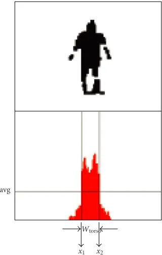
We assume that initially the human object stands straight up with his arms stretched as shown inFigure 3. The BDPs of the human model are illustrated in Table 1. The side viewer estimates the short radius of torso, whereas the front viewer determines the remaining parameters. The boundary of body, includingxleftmost,xrightmost,yhighest, andylowest, is
eas-ily found, as shown inFigure 4.
The front viewer estimates all BDPs except the short ra-dius of torso. There are three processes in the front viewer BDP determination: (a) torso-head-leg BDP determination, (b) arm BDP determination, and (c) fine tuning. Before the BDP estimation of the torso, head, and leg, we con-struct the vertical projection of the foreground image, that is, P(x)= f(x,y)d y, as shown inFigure 5. Then, we may find avg =xrightmost
xleftmost P(x)dx/(xrightmost−xleftmost), whereP(x)=0 forxleftmost < x < xrightmost.. To find the width of the torso,
we scanP(x) from left to right to findx1, the smallestxvalue
that makes P(x1) > avg, and then scanP(x) from right to
Table1: The BDPs to be estimated,Vindicates the existing BDP parameter.
Parameter Limb
Torso Head Upper arm Lower arm Upper leg Lower leg
Height V V V V V V
Radius — — V V — —
Long radius V V — — V V
Short radius V V — — V V
(a) (b)
Figure3: Initial posture of person: (a) the front viewer; (b) the side viewer.
xrightmost
xleftmost
ylowest
yhighest
xrightmost
xleftmost
ylowest
yhighest
Figure4: the BDPs estimation.
(seeFigure 5). Therefore, we may define the center of body asxc=(x1+x2)/2, and the width of torso,Wtorso=x2−x1.
To find the other BDP parameters, we remove the head by applying morphological filtering operations, which con-sists of the morphological closing operation using a structure element (size 0.8Wtorso ×1), and the morphological
open-ing operation by the same element (as shown in Figure 6). Then we may extract the location of shoulder iny-axis (yh)
by scanning the image (i.e.,Figure 6b) horizontally from top to bottom in the image without head, and define the length of head: lenhead= yhighest−yh. Here, we assume the ratio of
length of the torso and the leg is 4 : 6, and define the length of torso as lentorso=0.4(yh−ylowest); the length of upper leg
as lenup-leg=0.5×0.6(yh−ylowest), and the length of lower leg
as lenlow-leg=lenup-leg. Finally, we may estimate the center of
body iny-axis asyc=yh−lentorso; the long radius of torso as
LRtorso =Wtorso/2; the long radius of head as 0.2Wtorso; the
short radius of head as 0.16Wtorso; the long radius of leg as
0.2Wtorso; and the short radius of leg as 0.36Wtorso.
Before identifying the radius and length of arm, the system extracts the extreme position of arms, (xleftmost,yl)
and (xrightmost,yr) (as shown inFigure 7), and then defines
the position of shoulder joints, (xright-shoulder,yright-shoulder)=
(xa,ya)=(xc−LRtorso,yc−lentorso+0.45 LRtorso). From the
extreme position of arms and position of shoulder joints, we calculate the length of upper arm (lenupper-arm) and lower arm
(lenlower-arm), and the rotating angles around z-axis of the
shoulder joints (θarm
z ). These three parameters are defined
as follows: (a) lenarm =
(xb−xa)2+ (yb−ya)2; (b)θarmz =
arctan(|xb−xa|/|yb−ya|); (c) lenupper-arm =lenlower-arm =
lenarm/2. Finally, we fine-tune the long radius of torso, the
radius of arms, the rotating angles around thez-axis of the shoulder joints, and the length of arms.
To find the short radius of torso, the side viewer con-structs the vertical projection of the foreground image, that is,P(x)= f(x,y)d y, and avg=xrightmost
xleftmost P(x)dx/(xrightmost− xleftmost), whereP(x)=0 forxleftmost < x < xrightmost.
avg
x1 x2
Wtorso
Figure5: Foreground image silhouette and its vertical projection.
value, withP(x1)>avg, and then scanningP(x) from right to
left, we may also findx2, the largestxvalue, withP(x2)>avg.
Finally, the short radius of torso is defined as (x2−x1)/2.
3. MOTION PARAMETERS ESTIMATION
There are 25 motion parameters (22 angular parameters and 3 position parameters) for describing human body motion. Here, we assume that three rotation angles of head and two rotation angles of torso (rotation angle around X-axis and Z-axis) are fixed. The real-time tracking and motion estima-tion consists of four stages: (1) facade/flank determinaestima-tion, (2) Human position estimation, (3) arm joint angle estima-tion, and (4) leg joint angle estimation. In each stage, only the specific parameters are determined based on the match-ing between the model and the extracted object silhouette.
3.1. Facade/flank determination
First, we find the rotation angle of torso around the y-axis of the world coordinate (θT
YW). A y-projection of the fore-ground object image is constructed without the lower por-tion of the body, that is,P(x)=ymax
yhip f(x,y)d y, as shown in Figure 8. Each viewer finds the corresponding parameters in-dependently. Here, we define the hips’ position alongy-axis as yhip = (yc+ 0.2·heighttorso)·rt,n, where yc is the
cen-ter of body in y-axis, heighttorso is the height of torso, and rt,nis the perspective scaling factor of viewern(n=1 or 2),
which will be introduced in Section 4.2. Then, each viewer scansP(x) from left to right to find x1, the leastx, where
P(x1)>heighttorso, and then scansP(x) from right to left to
findx2, the largestx, whereP(x2)>heighttorso. The width of
the upper body isWu-body,n= |x2−x1|, wheren=1 or 2 is
the number of the viewer. Here, we define two thresholds for
each viewer to determine whether the foreground object is a facade view or a flank view:thlow,nandthhigh,n, wheren=1
or 2 is the number of the viewer. In viewern(n=1 or 2), if Wu-body,nis smaller thanthlow,n, it is a flank view; ifWu-body,n
is greater than thhigh,n, it is a facade view; otherwise, it
re-mains unchanged.
3.2. Object tracking
The object tracking determines the position, (XWT,YWT,ZWT),
of human object. We may simplify the perspective projection as a combination of the perspective scaling factor and the or-thographic projection. The perspective scaling factor values are calculated (inSection 4.2) by new positionXWT andZWT.
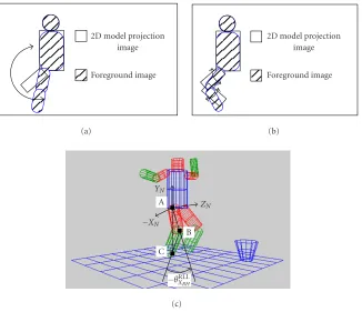
Given a scaling factor and BDPs, we generate a 2D model image. With the extracted object silhouette, we shift the 2D model image along X-axis in image coordinate and search for the realXT
W (orZTW in viewer 2) that generates the best
matching score, as shown inFigure 9a.
The estimatedXWT andZTW are then used to update the
perspective scaling factor for the other viewer. Similarly, we shift the silhouette alongY-axis in image coordinate to find YT
Wthat generates the best matching score (seeFigure 9b). In
each matching process, the possible position difference be-tween the silhouette and the model are−5,−2,−1, +1, +2, and +5. Finally, the positionsXWT andZWT are combined as
the 2D position values and a new perspective scaling factor can be calculated for the tracking process in the next time instance.
3.3. Arm joint angle estimation
The arm joint has 2 DOFs, and it can bend on certain 2D planes. In a facade view, we assume that the rotation an-gles of shoulder joint aroundX-axis of the navel coordinate (θXRUAN andθ
LUA
XN ) are fixed and then we may estimate the oth-ers includingθZRUAN ,θ RUA depicts the right upper arm, LUA depicts the left upper arm, RLA depicts the right lower arm, LLA depicts the left lower arm,Ndepicts the navel coordinate system,RSdepicts the right shoulder coordinate system, andLSdepicts the left shoulder coordinate system. to prevent the occlusion between the lower arms and the torso. In a flank view, the range ofθRUA
XN andθ
LUA
XN is limited in [−180◦, 180◦]. Here, we develop an overlapped tritree search method, see Section 3.5, to reduce the search time and ex-pand the search range. In a facade view, there are 3 DOFs for each arm joint, whereas in a flank view, there are 1 DOF for each arm joint. In a facade view, the right arm joint angle estimation is illustrated in the following steps.
(1) Determine the rotation angle of the right shoulder around theZ-axis of the navel coordinate (θRUA
(a)
ylowest
yh yhighest
(b)
Figure6: The head-removed image. (a) Result of closing. (b) Result of opening.
(xleftmost, yl) (xrightmost, yr)
(a)
Navel Torso
θarm
z
(xleftmost, yl) =(xb, yb)
Length of arm (lenarm)
(xright-shoulder, yright-shoulder)
=(xa, ya)
(b)
Figure7: (a) The extreme position of arms. (b) The radius and length of arm.
x2
x1 Heighttorso
yhip
(a)
x2
x1 Heighttorso
yhip
(b)
Figure8: Facade/flank determination. (a) Facade. (b) Flank.
(2) Define the range of the rotation angle of the right el-bow joint aroundx-axis in the right shoulder coordi-nate system (θXRLARS). It relies on the value of θ
RUA
ZN to
prevent the occlusion between the lower arm and the torso. First, we define a thresholdtha: ifθRUAZN >110
◦,
2D model projection
Figure9: Shift the 2D model image along (a)X-axis and (b)Y-axis.
2D model projection
Figure10: (a) Rotate upper arm alongZN-axis. (b) The definition oftha. (c) Rotate lower arm alongXRS-axis.
2D model projection image Foreground image
Figure11: Rotate the arm alongXN-axis.
So,θRLAXRS ∈[−tha, 140
(3) Determine the rotation angle of the right elbow joint around x-axis in the right shoulder coordinate sys-tem (θRLAXRS ) by applying the overlapped tritree search method and choose the value where the correspond-ing matchcorrespond-ing score is the highest (seeFigure 10c).
Similarly, in the flank view, the arm joint angle estima-tion determines the rotaestima-tion angle of shoulder around the X-axis of the navel coordinate (θXRUAN ) (seeFigure 11).
3.4. Leg joint angle estimation
The estimation processes for the joint angle of the legs in a facade view and a flank view are different. In a facade view, there are two cases depending on whether knees are bent or not. To decide which case, we check the location of navel in
y-axis to see whether it is less than that of the initial posture or not. If yes, then the human is squatting down, else he is standing. For the standing case, we only estimate the rota-tion angles of hip joints aroundZN-axis in navel coordinate
system (i.e.,θZRULN andθ
LUL
ZN ). As shown inFigure 12a, we esti-mateθRULZN by applying the overlapped tritree search method. In squatting down case, we also estimate the rotation an-gles of hip joints aroundZN-axis in navel coordinate system
(θRUL
ZN andθ
LUL
ZN ). After that, the rotation angles of the hip joints aroundXN-axis in the navel coordinate system (θXRULN andθLUL
XN ) and the rotation angles of the knee joints around xH-axis in the hip coordinate system (θXRLLRH andθ
LLL XLH) are es-timated. Because the foot is right beneath the torso,θRLL
XRH (or
XRHare estimated by applying a search method only forθRUL view, we estimate the rotation angles of the hip joints around xN-axis of the navel coordinate (θXRULN andθ
LUL
XN ) and the ro-tation angles of the knee joints around XH-axis of the hip
coordinates (θRLL
XRHandθ
LLL
XLH).
3.5. Overlapped tritree hierarchical search algorithm
2D model projection image
Foreground image
(a)
2D model projection image
Foreground image
(b)
−θRLL
XRH C
B A
−XN
ZN YN
(c)
Figure12: Leg joints angular values estimation in facade view. (a) Rotate upper leg alongZN-axis. (b) DetermineθXRULN andθ RLL
XRH. (c) The
definition ofθRLL
XRH.
Rr Rm
Rl
Search region
Figure13: The search region is divided into three overlapped sub-regions.
will be. Instead of using the sequential search in the specific search space, we apply the hierarchical search. As shown in Figure 13, we divide the search space into three overlapped regions (left region (Rl), middle region (Rm), and right
re-gion (Rr)) and select one search angle for each region. From
the three search angles, we do three different matches, and find the best match of which the corresponding region is the winner region. Then we update the next search region by the current winner region recursively until the width of the cur-rent search region is smaller than the step-to-stop criterion value. During the hierarchical search, we will update the win-ner angle if the current matching score is the highest. After reaching to the leaf of the tree, we assign the winner angle as the specific BAP.
We divide the initial search region R into three over-lapped regions asR =Rl+Rm+Rr, select the step-to-stop
criterion valueΘ, and do the overlapped tritree searching as follows.
(1) Letnindicate the current iteration index and initialize the absolute winning score asSWIN=0.
(2) Set θl,n as the left extreme of the current search
re-gionRl,n,θm,nas the center of the current search
re-gionRm,n, andθr,nas the right extreme of the current
search regionRr,n, and calculate the matching score
corresponding to the right region asS(Rl,n,θl,n), the
middle region asS(Rm,n,θm,n), and the left region as S(Rr,n,θr,n).
(3) If Max{S(Rl,n,θl,n),S(Rm,n,θm,n),S(Rr,n,θr,n)} < SWIN,
go to step (5), else Swin = Max{S(Rl,n,θl,n),S(Rm,n, θm,n),S(Rr,n,θr,n)}, θwin = θx,n|Swin=S(Rx,n,θx,n),x∈{r,m,l}, Rwin=Rx,n|Swin=S(Rx,n,θx,n),x∈{r,m,l}.
(4) Ifn = 1, thenθWIN = θwinandSWIN = Swin, else if
the current winner matching score is larger than the absolute winner matching score, Swin > SWIN, then
θWIN=θwinandSWIN=Swin.
(5) Check the width ofRwin, if|Rwin|>Θ, then continue,
else stop.
(6) DivideRwininto another three overlapped subregions:
Rwin = Rl,n+1+Rm,n+1+Rr,n+1 for the next iteration
n+ 1, and go to step (2).
On each stage, we may move the center of search region according to the range of joint angular value and the previous θwin, for example, when the range of arm joints is defined
as [0, 180] and the current search region’s width is defined as|Rarm-j| =64. If theθwinin the previous stage is 172, the
center ofRarm-jwill be moved to 148 (180−64/2=148) and
Rarm-j = [116, 180], so that the right boundary ofRarm-jis
the center ofRarm-jis unchanged,Rarm-j=[68, 132], because
the search region is inside the range of angular variation of the arm joint.
In each stage, the tritree search process compares the three matches and finds the best one. However, in real imple-mentation, it requires less matching because some matching operations in current stage had been calculated in the previ-ous stage. When the winner region in previprevi-ous stage is the right or left region, we only have to calculate the matches us-ing the middle point of current search region, and when the winner region in previous stage is the middle region, we have to calculate the matches using the left extreme and the right extreme of the current search region.
Here we assume that the winning probabilities of the left, middle, or right region are equiprobable. The number of matching of the first stage is 3 and the average number of matching in other stagesT2,avg=2×(1/3) + 1×(2/3)=4/3.
The average number of matching is
Tavg=3 +T2,avg·
whereWinitis the width of the initial search region andWsts
is the final width for the step to stop. The average number of matching for the arm joint is 3 + 4/3∗(6−2−1) =7 because Winit = 64 andWsts = 4. The average number of
matching operations for estimating the leg joint is 5.67(3 + 4/3∗(5−2−1)) becauseWinit=32 andWsts=4. The worst
case for the arm joint estimation is 3 + 2∗(6−2−1)=9 matching (or 3+2∗(5−2−1)=7 matching for the leg joint), which is better than the full search method which requires 17 matching for the arm joint estimation and 9 matching for the leg joint estimation.
4. THE INTEGRATION AND ARBITRATION OF TWO VIEWERS
The information integration consists of camera calibra-tion, 2D position and perspective scaling determinacalibra-tion, fa-cade/flank arbitration, and BAP integration.
4.1. Camera calibration
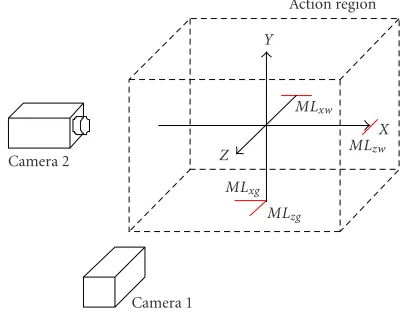
The viewing directions of two cameras are orthogonal. We define the center of action region as the origin in the world coordinate and we assume that the position of these two cameras are fixed at (Xc1,Yc1,Zc1) and (Xc2,Yc2,Zc2). The
viewing directions of these two cameras are parallel toz-axis andx-axis. Here we let (Xc1,Yc1)≈(0, 0) and (Yc2,Zc2)≈
(0, 0). The viewing direction of camera 1 points to the nega-tiveZdirection, while that of camera 2 points to the positive Xdirection. The camera is initially calibrated by the follow-ing steps.
(1) Fix the positions of camera 1 and camera 2 on thez -axis andx-axis.
(2) Put two sets of line markers on the scene (MLzg
andMLzw as well as MLxg andMLxw, as shown in Figure 14). The first two line markers are projection ofZ-axis onto the ground and the left-hand side wall. The second two line markers are the projection ofX -axis onto the ground and the background wall.
Camera 1
Figure14: The line marker for camera calibration.
(3) Adjust the viewing direction of camera 1 until the line markerMLzgoverlaps the linex=80 and the linex=
81; the line markerMLxwoverlaps the liney=60 and
the liney=61.
(4) Adjust the viewing direction of camera 2 until the line markMLxgoverlaps the linex =80 and the linex =
81; the line markerMLzwoverlaps the liney=60 and
the liney=61.
The camera parameters include the focal lengths and the positions of the two cameras. First we assume that there are three rigid objects located at the positions A = (0, 0, 0),
B = (0, 0,DZ), andC=(DX, 0, 0) in the world coordinate,
where DX andDZ are known. Therefore, the pinnacles of
three rigid objects are located at positions A,B, and C, where theA =(0,T, 0),B =(0,T,DZ), andC =(DX,T, 0)
in the world coordinate. The pinnacles of the three rigid ob-jects are projected at (x1A,t1A), (x1B,t1B), and (x1C,t1C) in
the image frame of camera 1, and (z2A,t2A), (z2B,t2B), and
(z2C,t2C) in the image frame of camera 2, respectively.
We assume λ1 is the focal length of camera 1, and
(0, 0,Zc1) is its location. By applying the triangular
geom-etry calculation on perspective projection images, we have λ1 = Zc1(x1c −x1A)/Dz. Similarly, let λ2 the focal length
and (Xc2, 0, 0) the location of camera 2, and we haveλ2 = −Xc2(z2B−z2A)/Dz.
4.2. Perspective scaling factor determination
The location of the object is (XT
W,YWT,ZWT) in the world
co-ordinate, of which theXT
WandZWT can be obtained from two
viewers. Here, we need to find the depth information and calculate the perspective scaling factors of these two viewers. Here, we assume that the location of the object changes from
A = (0, 0, 0) to D = (DX , 0,DZ ),Xc1 ≈ 0, andZc2 ≈ 0.
The pinnacle of the object moves from A = (0,T, 0) to
D =(DX ,T ,DZ ). The ratioT /Tis not a usable parameter
because it is depth dependent and there is a great possibility that human object may be squatting down. The pinnacles of the previous and current objects are projected as (x1A,t1A)
and (x1D ,t1D ) in camera 1, and as (z2A,t2A ) and (z2D ,t2D )
they are depth dependent, however, the locations,x1D and z2D are approximated asx1D ≈XWT andz2D ≈ZWT. The
perspective scaling factors of human model in two viewers (i.e.,rt1 andrt2) are different, wherert1 = |t1D /t1A |and
and then find the perspective scaling factorrt1 andrt2 as
rt1=
The highest pixel of the silhouette is treated as the top of the object and each position of the silhouette object is approxi-mated to be that of the human object. Using perspective scal-ing factor, we may scale our human model for the followscal-ing BAP estimation process.
The side viewer estimates the short radius of torso, while the front viewer finds the remaining parameters. During ini-tialization, the height of human object ist1in viewer 1 andt2
in viewer 2, so the scaling factor between the viewers isrt = t2/t1. Therefore, the BDPs of human models for viewer 1 and
viewer 2 can be easily scaled. Because the universal BDPs are defined in the scaling factor of viewer 1, we define the short radius of torso in universal BDPs asSRtorso,u = SRtorso,2/rt,
whereSRtorso,2is the short radius of torso in viewer 2 and the
remaining parameters in universal BDPs are defined directly as those in viewer 1.
4.3. Facade/flank arbitrator
The facade/flank arbitrator combines the results of fa-cade/flank transition processes of the two viewers. Initially, viewer 1 is the front viewer and captures the facade view of the object, whereas viewer 2 is the side viewer and cap-tures the flank view of the object. Then, when either viewer 1 or viewer 2 changes their own facade/flank transitions, then they will ask the facade/flank arbitrator for coordination. If any one of the following transitions occurs, the facade/flank arbitrator will perform the corresponding coordination as follows.
(1) When the object in viewer 1 changes from flank to fa-cade (i.e.,wu-body,1 > thhigh,1) and the same object in
viewer 2 stays as facade (i.e.,wu-body,2 ≥ thlow,2), the
arbitrator checks as follows: if|wu-body,1−thhigh,1| > |wu-body,2−thlow, 2|, then sets the object in viewer 2 to flank, else changes the object in viewer 1 back to flank.
(2) When the object in viewer 1 changes from facade to flank (i.e.,wu-body,1 < thlow,1) and the same object in
viewer 2 stays as flank (i.e.,wu-body,2 ≤ thhigh,2), the
arbitrator checks as follows: if|wu-body,1−thlow,1| > |wu-body,2−thhigh,2|, then sets the object in viewer 2 to
facade, else changes the object in viewer 1 back to facade. (3) When the object in viewer 1 remains as facade (i.e., wu-body,1 ≥ thlow,1) and the same object in viewer 2
changes from flank to facade (i.e.,wu-body,2> thhigh,2),
the arbitrator checks as follows: if|wu-body,1−thlow,1| ≥ |wu-body,2−thhigh,2|, then sets the object in viewer 2 back
to flank, else changes the object in viewer 1 to flank. (4) When the object in viewer 1 stays as flank (i.e.,
wu-body,1 ≤ thhigh,1) and the same object in viewer 2
changes from facade to flank (i.e.,wu-body,2 < thlow,2),
the arbitrator checks as follows:if|wu-body,1−thhigh,1| ≥ |wu-body,2−thlow,2|, then sets the object in viewer 2 back
to facade, else changes the object in viewer 1 to facade.
4.4. Body animation parameter integration
Two different sets of BAPs have been estimated by the two viewers. There are three major estimation processes for BAPs: human position estimation, arm joint angle estimation, and leg joint angle estimation. The BAP integration combines the BAPs from two different views into universal BAPs. First, in human position estimation, viewer 1 estimatesXWT andYWT,
while viewer 2 estimatesZWT andYWT. However,YWT estimated
by two viewers may be different. With more shape informa-tion of the object,YT
Westimated by the facade viewer is more
robust. Second, the BAPs of the joints of arms are analyzed in two views. The flank viewer only estimates the rotation angles of shoulder joints aroundXN-axis of the navel
coor-dinate (i.e.,θRUA
XN andθ
LUA
XN ); whereas the facade viewer esti-mates the other BAPs of arms including the rotation angles of shoulder joints around YN-axis andZN-axis of the navel
coordinate (i.e.,θRUAYN ,θ angles of elbow joints around XN-axis of shoulder
coordi-nates (i.e.,θRLA
XN andθ
LLA
XN ). BAPs estimation processes of the two viewers are integrated as the universal BAPs.
Different from the integration of the arm BAPs, the es-timated joint angles of leg of different viewers are related. Both viewers jointly estimateθRULXN ,θ
RLL example, inFigure 15, the facade viewer analyzes these an-gles by assuming that the human is squatting down (see Fig-ures15aand15b); whereas the flank viewer estimates these angles by assuming that the human is lifting his legs (see Figures15cand15d). Therefore, we determine whether the human is squatting down or lifting his leg from θZRULN and θRLLXRH.
IfθZRULN (from the facade viewer) is greater than 175 ◦but less than 180◦, the human is lifting his right leg, else he is not. Then, we may integrateθRUL
ZN (from the facade viewer),θ
RUL
XN (from the flank viewer), and θRLL
2D model projection image
Foreground image
θRLL
XRH
θRUL
XN
(a) (b)
2D model projection image
Foreground image
θRULXN
2D model projection image
Foreground image
θRLLXRH
(c)
(d)
Figure15: The facade viewer and the flank viewer estimateθRUL
XN ,θ RLL
XRH,θ LUL
XN , andθ LLL
XRH. (a) Squatting down (the facade view).
(b) Virtual actor is squatting down. (c) Leg lifting (the facade view). (d) Virtual actor is lifting his leg.
5. EXPERIMENTAL RESULTS
The color image frame is 160×120×24 bits and the frame rate is 15 frames per second. Each test video sequence lasts more than 2 seconds, so that it may consist of about 40 frames. We use two computers equipped with video capturing equip-ment. Our system analyzes and estimates the BAPs of human motion in real time, based on the matching between the ar-ticulated human model and the 2D binary human object. In the experiments, we illustrate 15 human postures composed of the following five basic movements: (1) walking; (2) arm raising; (3) arm swing; (4) squatting; (5) kicking. To evalu-ate the performance of our tracking process, we test the
sys-tem by using 15 different human motion postures. Each one is performed by 12 different individuals. People with casual wear and no markers are instructed to perform 15 different actions as shown inFigure 16.
Table2: The number of correct recognitions for each posture.
Posture 1 2 3 4 5 6 7 8 9 10 11 12 13 14 15
Correct Recognition 22 21 23 21 24 20 23 24 22 22 23 24 21 22 20
Model 1
P(O|Model 1)
Model 2
P(O|Model 2)
. . .
ModelN P(O|ModelN) Test
image
BAP estimation
Maximum selection
Figure17: The evaluation system.
5.1. Training phase
A set of the joint angles (i.e., BAPs) have been extracted from each video frame which are combined as a so-called feature vector. A feature vector will be assigned to an observation or to a symbol. To train the HMMs, we need to determine some parameters: the observation number, the state number, and the dimension of the feature vector. There is a tradeoff between selecting a large observation number and a faster HMM computation. A larger one means more accurate ob-servations and more computation. From the experiments, we choose 64 symbols. The issue of the number of states also needs to be determined. The states are not necessarily corre-sponding to the physical observations of the correcorre-sponding process. The number of states and the number of the differ-ent postures in human motion sequences are related. Here, we develop the 5-state HMM, which is most suitable for our experiments.
The tracking process has estimated the joint angles of the human actor, and there are 17 joint angles for the human model. Actually, not all of the joint angles are required for describing different postures. Hence, we only choose some influential joint angles representing the postures, such as the joint anglesθxandθzof the shoulders,θxof the elbows, and θxandθz of the hips. Totally, 10 joint angles are selected as
one feature vector. Here, we need to train 15 HMMs corre-sponding to 15 different postures. The training process will generate the model parameterλifor theith HMM.
5.2. Recognition phase
In our experiments, there are 360 testing sequences for per-formance evaluation. There are 15 different human postures, and each one is performed twice by 12 different individuals.
As shown inFigure 17, every testing sequence,O, is evaluated by 15 HMMs. The likelihood of the observation sequences can be computed for each HMM asPi=log(P(O|λi)), where λiis the model parameter of theith HMM. The HMM with
maximum likelihood is selected to represent the recognized posture which is currently performed by the human actor in the test video sequence.
The experimental results are shown inTable 2. Each pos-ture is tested 24 times by 12 different individuals. The recog-nition errors are caused mainly by the incorrect BAPs. The BAP estimation algorithm may fail if the extracted fore-ground object is noisy or ambiguous, which is caused by the occlusion between the limbs and the torso. The limitation of our algorithm can be summarized as follows.
(1) Since the BAP estimation is based on the preceding BAP in the previous time instance, the error propaga-tion cannot be avoided. Once the error of the previous BAP is above certain level, the search range for the fol-lowing BAP no longer covers the correct BAP, and the system may crash.
(2) The occlusion of human body is the major challenge for our algorithm. By using two views, some occlusion in one view should be clear in the other view. However, if the arm is swing beside the torso, it makes occlu-sion in both the facade and flank views. The occluocclu-sion among the limbs and the torso will make BAP estima-tion fail, since the matching process cannot differenti-ate the limb from the torso in the silhouette image. (3) Arm swing is another difficult issue. The side viewer
cannot differentiate whether one arm or two arms is being raised. The silhouette of the arm swing viewed from the front view is not very reliable for accurate an-gle estimation.
(4) It cannot tell if a facade is a front view or just a back view. We may add the face-finding algorithm to iden-tify whether the human actor is facing toward the cam-era or not.
6. CONCLUSION AND FUTURE WORKS
REFERENCES
[1] G. Johansson, “Visual motion perception,” Scientific Ameri-can, vol. 232, no. 6, pp. 76–89, 1975.
[2] A. G. Bharatkumar, K. E. Daigle, M. G. Pandy, Q. Cai, and J. K. Aggarwal, “Lower limb kinematics of human walking with the medial axis transformation,” inProc. IEEE Workshop on Mo-tion of Non-Rigid and Articulated Objects, pp. 70–76, Austin, Tex, USA, November 1994.
[3] Y. Li, S. Ma, and H. Lu, “A multiscale morphological method for human posture recognition,” inProc. IEEE International Conference on Automatic Face and Gesture Recognition, pp. 56– 61, Nara, Japan, April 1998.
[4] M. K. Leung and Y.-H. Yang, “First sight: a human body out-line labeling system,”IEEE Trans. on Pattern Analysis and Ma-chine Intelligence, vol. 17, no. 4, pp. 359–377, 1995.
[5] J. O’Rourke and N. I. Badler, “Model-based image analysis of human motion using constraint propagation,”IEEE Trans. on Pattern Analysis and Machine Intelligence, vol. 2, no. 6, pp. 522–536, 1980.
[6] K. Sato, T. Maeda, H. Kato, and S. Inokuchi, “CAD-based ob-ject tracking with distributed monocular camera for security monitoring,” inProc. 2nd CAD-Based Vision Workshop, pp. 291–297, Champion, Pa, USA, February 1994.
[7] D. Marr and H. K. Nishihara, “Representation and recogni-tion of the spatial organizarecogni-tion of three-dimensional shapes,” Proc. Roy. Soc. London. Ser. B., vol. 200, no. 1140, pp. 269–294, 1978.
[8] T. B. Moeslund and E. Granum, “A survey of computer vision-based human motion capture,” Computer Vision and Image Understanding, vol. 81, no. 3, pp. 231–268, 2001.
[9] K. Tamagawa, T. Yamada, T. Ogi, and M. Hirose, “Developing a 2.5-D video avatar,” IEEE Signal Processing Magazine, vol. 18, no. 3, pp. 35–42, 2001.
[10] K. Rohr, “Human movement analysis based on explicit mo-tion models,” in Motion-Based Recognition, M. Shah and R. Jain, Eds., vol. 9 ofComputational Imaging and Vision, chapter 8, pp. 171–198, Kluwer Academic Publishers, Boston, Mass, USA, 1997.
[11] C. R. Wren, A. Azarbayejani, T. Darrell, and A. Pentland, “Pfinder: real-time tracking of the human body,”IEEE Trans. on Pattern Analysis and Machine Intelligence, vol. 19, no. 7, pp. 780–785, 1997.
[12] I. Haritaoglu, D. Harwood, and L. S. Davis, “W4: Real-time
surveillance of people and their activities,”IEEE Trans. on Pat-tern Analysis and Machine Intelligence, vol. 22, no. 8, pp. 809– 830, 2000.
[13] I. Haritaoglu, D. Harwood, and L. S. Davis, “A fast back-ground scene modeling and maintenance for outdoor surveil-lance,” inProc. IEEE 5th International Conference on Pattern Recognition (ICPR ’00), vol. 4, pp. 179–183, Barcelona, Spain, September 2000.
[14] Q. Cai and J. K. Aggarwal, “Automatic tracking of human motion in indoor scenes across multiple synchronized video streams,” inProc. IEEE Sixth International Conf. on Computer Vision (ICCV ’98), pp. 356–362, Bombay, India, January 1998. [15] D. M. Gavrila and L. S. Davis, “3-D model-based tracking of humans in action: a multi-view approach,” inProc. IEEE Computer Society Conference on Computer Vision and Pattern Recognition (CVPR ’96), pp. 73–80, San Francisco, Calif, USA, June 1996.
[16] R. Cutler and L. Davis, “Robust real-time periodic motion detection, analysis, and applications,” IEEE Trans. on Pattern Analysis and Machine Intelligence, vol. 22, no. 8, pp. 781–796, 2000.
[17] Y. Ricquebourg and P. Bouthemy, “Real-time tracking of mov-ing persons by exploitmov-ing spatio-temporal image slices,”IEEE Trans. on Pattern Analysis and Machine Intelligence, vol. 22, no. 8, pp. 797–808, 2000.
[18] A. Nkazawa, H. Kato, and S. Inokuchi, “Human tracking us-ing distributed vision system,” inProc. IEEE 14th International Conference on Pattern Recognition (ICPR ’98), vol. 1, pp. 593– 596, Brisbane, Australia, August 1998.
[19] A. Utsumi, H. Yang, and J. Ohya, “Adaptive human motion tracking using non-synchronous multiple viewpoint observa-tions,” inProc. IEEE 15th International Conference on Pattern Recognition (ICPR ’00), vol. 4, pp. 607–610, Barcelona, Spain, September 2000.
[20] S. Iwasawa, J. Takahashi, K. Ohya, K. Sakaguchi, T. Ebihara, and S. Morishima, “Human body postures from trinocular camera images,” inProc. 4th IEEE International Conference on Automatic Face and Gesture Recognition, pp. 326–331, Greno-ble, France, March 2000.
[21] C. Bregler, “Learning and recognition human dynamics in video sequrence,” inProc. IEEE Computer Society Conference on Computer Vision and Pattern Recognition (CVPR ’97), pp. 568–574, Puerto Rico, June 1997.
[22] I.-C. Chang and C.-L. Huang, “The model-based human body motion analysis system,” Image and Vision Computing, vol. 18, no. 14, pp. 1067–1083, 2000.
[23] M. Brand and V. Kettnaker, “Discovery and segmentation of activities in video,” IEEE Trans. on Pattern Analysis and Ma-chine Intelligence, vol. 22, no. 8, pp. 844–851, 2000.
[24] N. Krahnstover, M. Yeasin, and R. Sharma, “Towards a unified framework for tracking and analysis of human motion,” in Proc. IEEE Workshop on Detection and Recognition Events in Video, pp. 47–54, Vancouver, Canada, July 2001.
Chung-Lin Huangwas born in Tai-Chung, Taiwan, in 1955. He received his B.S. de-gree in nuclear engineering from the Na-tional Tsing-Hua University, Hsin-Chu, Tai-wan, in 1977, and his M.S. degree in electri-cal engineering from National Taiwan Uni-versity, Taipei, Taiwan, in 1979, respectively. He obtained his Ph.D. degree in electrical engineering from the University of Florida, Gainesville, Fla, USA, in 1987. From 1981
to 1983, he was an Associate Engineer in ERSO, ITRI, Hsin-Chu, Taiwan. From 1987 to 1988, he worked for the Unisys Co., Orange County, Calif, USA as a project engineer. Since Au-gust 1988, he has been with the Department of Electrical Engi-neering, National Tsing-Hua University, Hsin-Chu, Taiwan. Cur-rently, he is a Professor in the same department. His research interests are in the area of image processing, computer vision, and visual communication. Dr. Huang is a Member of IEEE and SPIE.