Stability and evolution of the climate system of Mars
Takasumi Nakamura and Eiichi Tajika
Department of Earth and Planetary Science, The University of Tokyo, 7-3-1 Hongo, Bunkyo-ku, Tokyo 113-0033, Japan
(Received December 4, 2000; Revised April 14, 2001; Accepted April 17, 2001)
We construct a one-dimensional energy balance climate model for Mars which incorporates greenhouse effect of CO2and latitudinal heat transport so that we can express a latitudinal temperature gradient and change of an
areal extent of a polar ice cap. By considering energy balance and CO2 budget among atmosphere, ice caps, and
regolith, we investigate stability and evolution of the climate system of Mars. Under the present condition there are two stable steady state solutions of the system. One corresponds to a partial ice-covered solution (the present state), and the other is a warmer ice-free solution. Although this is also predicted by previous studies, these solutions are qualitatively different from them. When we assume CO2as a dominant greenhouse gas for a warm and wet climate
on the early Mars, we found that the total amount of CO2within the whole system should have been larger than that
at present and have decreased by some removal processes. We also found that a climate jump must have occurred during the evolution from the early warm climate to the present state, and ice caps on the early Mars might have extended to the mid-latitude. The atmospheric pressure may have decreased further after the climate jump.
1.
Introduction
Ever since Mariner 9 and Vikings found many valleys and basins on the surface of Mars, Martian paleoenvironment under which these topographies were created has been dis-cussed. Valley networks and traces of possible paleoshore-lines on the Martian surface are regarded as possible evi-dence of existence of liquid water during the early history of Mars (e.g., Goldspiel and Squyres, 1991; Baker et al., 1992; Headet al., 1999). The low elevation of the northern hemisphere and its flatness might also imply that the north-ern hemisphere was once covered with a vast ocean (Smith et al., 1998). These features suggest that the ancient Mars might have warm and wet environment. Because solar lu-minosity was lower in the past than at present (Sagan and Mullen, 1972), it is likely that strong greenhouse effect due to some greenhouse gas species should have worked at that time to make warm environment on the ancient Mars. It was generally believed that the Martian atmosphere was reducing early in its history. However, it has been shown that reduc-ing gases (such as CH4and NH3) are photochemically
un-stable (Kuhn and Atreya, 1979). It is now believed that CO2
was the dominant greenhouse gas in the early atmosphere of Mars, although other possibilities such as greenhouse effect of CH4 and/or NH3 cannot be excluded entirely (Kasting,
1997; Sagan and Chyba, 1997).
There are several controlling mechanisms for the atmo-spheric CO2pressure on Mars. For instance, if there was
liq-uid water (oceans or ponds) under warm and wet conditions, CO2must have removed from the atmosphere by chemical
weathering of silicate rocks followed by precipitation of car-bonate (Pollacket al., 1987; Bakeret al., 1991). Even if the
Copy right cThe Society of Geomagnetism and Earth, Planetary and Space Sciences (SGEPSS); The Seismological Society of Japan; The Volcanological Society of Japan; The Geodetic Society of Japan; The Japanese Society for Planetary Sciences.
surface temperature was below the freezing point of water, large impacts could have removed a part of the atmosphere during the heavy bombardment period (Melosh and Vickery, 1989). Escape of atmospheric CO2by ion sputtering is also
suggested to have occurred throughout the history of Mars (Luhmann et al., 1992). On the other hand, volcanic de-gassing might have supplied CO2to the atmosphere (Baker
et al., 1991). It is also important to consider the polar ice caps (e.g., Leighton and Murray, 1966) and the surface re-golith (Fanale and Cannon, 1974) which might have been large CO2reservoirs to exchange CO2with the atmosphere.
Gierasch and Toon (1973) assumed the atmosphere and the polar ice caps as dominant CO2reservoirs. They studied
multiple solutions for a model of the atmosphere-ice cap (AI) system and analyzed stability of the solutions. They used a zero-dimensional energy balance climate model, although they assumed the winter polar region and the low-latitude region and considered heat transport between them due to baroclinic instability. They found that the AI system has two stable solutions: one is the present state and the other is the warmer state with higher CO2pressure.
On the other hand, McKayet al.(1991) assumed the at-mosphere and the regolith as dominant CO2reservoirs, and
studied multiple solutions for the atmosphere-regolith (AR) system and stability of solutions. They combined a one-dimensional radiative-convective model proposed by Pollack et al.(1987) with a model for CO2exchange between the
re-golith and the atmosphere proposed by Toonet al.(1980). They argued that the AR system may have two stable states, depending on sensitivity of CO2 adsorption by the regolith
to the surface temperature. One of them is the present state, and the other is the warmer state with higher CO2pressure.
These two studies, however, may have some problems. Gierasch and Toon (1973) did not consider the greenhouse
effect of CO2 and adsorption of CO2 by the regolith, and
assumed the polar cap to be an infinite CO2 reservoir with
no areal extent. On the other hand, McKayet al.(1991) did not consider roles of CO2-ice caps as a CO2reservoir which
may regulate the atmospheric CO2pressure and as a reflector
of incident solarflux, especially in the distant past.
Haberleet al.(1994) modified the energy balance model of Gierasch and Toon (1973) to study the evolution of CO2on
Mars from the end of the heavy bombardment period to the present by considering chemical weathering, regolith uptake, polar cap formation, and atmospheric escape by sputtering. They argued that the polar caps could have profound effect on behavior of the system: once ice caps were formed, the volume of ice caps increases drastically owing to a feedback effect between surface pressure, greenhouse effect, and heat transport, resulting in a collapse (catastrophic reduction) of the atmosphere. However, they did not discuss multiplicity of the steady state solutions and stability of them, and, because their model is also zero-dimensional, they could not consider areal extent of polar caps which should affect both the energy balance and the condition for ice cap formation.
In this paper, we investigate stability and property of steady state solutions of the Martian climate system. We consider an atmosphere-ice cap-regolith (AIR) system as a climate sys-tem of Mars. According to Hoffertet al.(1981) and Postawko and Kuhn (1986), atmospheric heat transport controls sur-face temperature profile, hence areal extent of the CO2caps.
Therefore, we construct a one-dimensional energy balance climate model combined with greenhouse effect of CO2and
latitudinal heat transport so that we can express a latitudinal temperature gradient and a change of the areal extent of polar ice caps explicitly. By considering both the energy balance and the CO2budget, we examine the steady state and
stabil-ity of the AIR system. Possible scenarios for the evolution of Martian climate system will be also discussed.
2.
Model
We introduce a one-dimensional energy balance climate model (1-D EBM) based on Northet al.(1981). It is, how-ever, noted that the model must be modified in order to de-scribe the climate system of Mars which is quite different from that of the Earth. In this study, we assume annual mean conditions and symmetrical hemispheres in order to compare the previous zero-dimensional annual mean model. The CO2
ice sheet expands from the pole to a certain latitude (this ice cap edge is called“iceline”), and there is no ice from the iceline to Equator.
The 1-D EBM is an energy balance model that can ex-press latitudinal heat transport. In a steady state, the en-ergy balance at the surface of thei-th latitude is represented as [Net horizontal heat transport out]i+[Outgoing infrared
radiation]i =[Incident solar radiation absorbed]i. This may
be represented mathematically by the relation
− ∂ whereD is a thermal diffusion coefficient,x is the sine of latitude (that is,x =sinφwhereφis the latitude),xs
cor-responds to the iceline,T(x)is the surface temperature in a given latitude band,I(x)is the outgoing infrared radiation,
Qis the solar constant at the orbit of the planet,S(x)is the annual mean solar income distribution, andais the planetary albedo. In this study, we assume the present solar income distribution as follows (Hoffertet al., 1981).
S(x)=1.235−0.693x2. (2)
The boundary conditions for symmetric solutions are given by
−D1−x2∂T(x)
∂x =0 forx=0,1. (3)
The planetary albedoa(x,xs)is expressed as follows.
a(x,xs)=
af for 0<x<xs
ai forxs≤x<1. (4)
We assumedaf =0.21 as the surface albedo of land (Pollack et al., 1987), andai =0.65 as CO2ice (Leighton and Murray,
1966).
One of the most important problem to study the stability of CO2atmosphere is condensation of CO2to form CO2clouds
(Kasting, 1991). Kasting (1991) argued that condensation of CO2should release latent heat and so decreases the lapse
rate, resulting in a decrease in the surface temperature in or-der to maintain energy balance. The CO2 cloud is a good
scatterer for solar radiation, thus it should increase the plan-etary albedo. Condensation of CO2 may limit the amount
of atmospheric CO2 when the entire atmosphere is covered
with CO2cloud.
Recently, Forget and Pierrehumbert (1997) argued that CO2 ice particle larger than 10μm can scatter infrared
ra-diation back to the surface. They included this effect in the 1-D radiative-convective model designed for early Mars by Kasting (1991), and showed that greenhouse effect of CO2
cloud could be quite powerful. Although magnitude of the greenhouse effect of CO2 cloud should depend on fraction
of cloud cover and optical thickness, these properties have not been known. Therefore, the effect of CO2clouds on the
energy balance may have been still unclear.
In this study, we adopt a traditional expression of outgoing infrared radiation I(x) which is approximated to a linear function ofT(x)as follows:
I(x)=A+BT(x). (5)
The coefficients Aand B depend on the atmospheric CO2
pressure. We determined these coefficients on the basis of the radiative-convective calculations by Pollacket al.(1987) which include greenhouse effects of CO2and H2O. Although
the model of Pollacket al.(1987) neglects H2O clouds,
ef-fects of H2O clouds should be small when the surface
tem-perature is below 273 K (the condition considered mainly in this study). Their model also neglects effects of the CO2
clouds. However, we will also discuss the case for CO2cloud
formation (Kasting, 1991; Forget and Pierrehumbert, 1997) in the later section. We parameterize A and B as a func-tion ofρ(=logPair: Pairis the surface pressure of CO2(in
as follows:
I =
A1+B1T forT >T0
A2+B2T forT ≤T0
(6)
A=a1ρ4+a2ρ3+a3ρ2+a4ρ+a5(W/m2)
B=b1ρ4+b2ρ3+b3ρ2+b4ρ+b5(W/m2K).
(7)
Fitting parameters (a1 ∼a5,b1 ∼b5, andT0) are shown in
Table 1.
According to Gierasch and Toon (1973), we assume that heat is transported meridionally by baroclinic instability. We adopt the parameterization of Stone (1972) for vertically in-tegrated heatflux which is expressed as a linear function of surface pressure. We also assume thatDis independent of latitude. Then we obtain
D=αPair (8)
whereαis a constant which is determined by the present-day condition.
The atmospheric pressure of CO2 should change owing
to changes in the areal extent of ice caps and the amount of CO2adsorbed in the regolith. The amount of CO2adsorbed
in the regolith (Prego) is represented by the equation used in
McKayet al.(1991). However, we modify their expression to consider latitudinal dimension as follows:
Prego =C
xs
0
e−T(x)/TdPγ
aird x (9)
whereC is a constant normalized by depth of the regolith, andTdandγ are parameters that determine the response of adsorption to surface temperature and pressure, respectively. The values of these parameters are adopted from McKayet al.(1991).
The amount of CO2as polar ice caps (Pice) is estimated
from the areal extent of ice caps and assumed CO2content in
ice caps per unit area. The latitude of iceline is determined from the temperature distribution obtained from the energy balance. The condition for the surface temperature at the iceline is defined here as
T(xs)=Tsub(Pair) (10)
whereTsub represents freezing point of CO2 as a function
of the atmospheric pressure. Although CO2 ice disappears
in summer on the north pole while it remains throughout the year on the south pole on Mars at present (Jameset al.,
Table 1. Fitting parameters for greenhouse model of Pollacket al.(1987). T0=230.1 K
i ai(A1) ai(A2) bi(B1) bi(B2)
1 0.6449 0.1068 −0.003256 −0.00094
2 13.28 2.198 −0.06758 −0.0195
3 99.54 16.48 −0.5069 −0.1464
4 329.9 54.64 −1.68 −0.485
5 −372.7 −61.72 1.898 0.5479
1992; Tanaka and Abe, 1991), we assume symmetry of hemi-sphere for simplicity. It is noted that the correct amount of this reservoir may have been still unclear. According to the previous studies, the amount of CO2in the ice-cap reservoir
is estimated to be from several mbars (Fanaleet al., 1982) to<254 mbars (more realistically, <a few tens of mbars) (Mellon, 1996). Therefore, the amount of CO2in the ice-cap
reservoir may be less than a few tens of mbars, or, at least, several mbars. In this study, we assume annually averaged expansion of the CO2caps to be as far as 70◦ for both caps
with a thickness of 25 m, then we obtain Pice = 85 mbar
for a nominal current condition. The value we used can be regarded as an upper estimate for the CO2ice-cap reservoir.
When we give the total amount of CO2 contained in the
AIR system (Ptotal), that is,
Ptotal=Pair+Pice+Prego (11)
we can obtain steady state solutions for the system by solv-ing the energy balance and the CO2 exchange among the
reservoirs.
3.
Results
3.1 Steady state solutions of the 1-D EBM
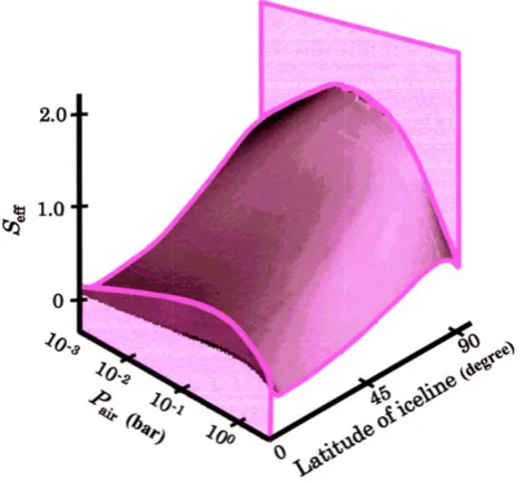
In this section, we show steady state solutions of the 1-D EBM and discuss some specific features. Figure 1 shows steady state solutions of the 1-D EBM (Eqs. (1)∼(8), and (10)) expressed as a curved surface of
Seff≡
Q Q0
= f(Pair, φs) (12)
whereSeff is an effective solar constant andQ0is the solar
constant at the Martian orbit today. Steady state solutions of the AIR system (Eqs. (1)∼(11)) exist on this curved surface. Figure 2(a) is a plane ofφs =90◦(Pair–Seffplane) of Fig. 1.
The region above the curve is the ice-free solutions, and there is no solution below the curve. Figure 2(b) is a projection
Fig. 2. Cross sections of Fig. 1. (a) A plane ofφs =90◦. The region above the curve is the ice-free solutions. The sign of∂Seff/∂Pairchanges becausePairaffects both the greenhouse effect and the freezing point of CO2. (b) The projection of the solutions ontoPair–φsplane. (c) A plane ofφs=0◦. The region below the curve is the ice-covered solutions.
of Fig. 1 onto Pair–φsplane. Figure 2(c) is a plane ofφs =
0◦(Pair–Seff plane). The region below the curve is the
ice-covered solutions, and there is no solution above the curve. In the climate system of the Earth, there exists ice albedo feedback which is a positive feedback mechanisms derived from albedo difference between land and ice caps (Budyko, 1969). In the Martian climate system, however, additional three feedbacks with respect to CO2ice caps will exist; (1)
increase in the atmospheric CO2pressure due to decrease in
the ice caps and decrease in the amount of CO2adsorbed in
the regolith should result in increase in the greenhouse effect and further decrease in the ice caps (this represents a posi-tive feedback), (2) increase in the atmospheric CO2pressure
due to decrease in the ice caps and in the amount of CO2
adsorbed in the regolith should result in increase in freez-ing point of CO2, which prevents the ice caps from
reduc-ing (this represents a negative feedback). We name (1) and (2) “greenhouse feedback”and“freezing point feedback”, respectively. Another feedback mechanism is (3) a “heat transport feedback”. Change in the atmospheric CO2
pres-sure should change efficiency of the latitudinal heat trans-port. When Pair increases, the efficiency of the latitudinal
heat transport increases. Then, if the net budget of latitu-dinal heat transport is positive at the iceline (that is, higher latitude region), the polar caps should shrink. This is a pos-itive feedback mechanism. On the other hand, if the net budget of latitudinal heat transport is negative at the iceline (that is, lower latitude region), the polar caps should expand. In this case, it represents a negative feedback mechanism. This negative feedback was not taken into account in the previous models of Gierasch and Toon (1973) and Haberle
et al.(1994), because the ice cap could not extend to lower latitude region in their models.
It is noted that signs of ∂Seff/∂φs, ∂Seff/∂Pair, and
∂φs/∂Pair change along the solution surface (Fig. 1). The
sign of∂Seff/∂φschanges because of the ice albedo feedback
(Northet al., 1981). On the other hand, signs of∂Seff/∂Pair
and∂φs/∂Pairare determined by relative strength of two
feed-back effects: freezing point feedfeed-back is stronger than green-house feedback where∂Seff/∂Pair >0 and∂φs/∂Pair <0.
This is because, in that region, the ice cap becomes large owing to the higher freezing point when the atmospheric pressure becomes high. On the other hand, greenhouse feed-back is stronger where∂Seff/∂Pair <0 and∂φs/∂Pair >0.
This is because, in that region, the ice cap becomes small ow-ing to the stronger greenhouse effect when the atmospheric pressure becomes high (see Fig. 2).
3.2 Solutions under the current condition
Next, we show the steady state solutions of the 1-D EBM coupled with the AIR system (Eqs. (1)∼(11)). Martian sur-face condition at present is given as boundary condition. Standard values of the parameters are shown in Table 2.
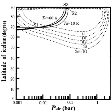
Figures 3 and 4 show the numerical results. In Fig. 3, the solutions are projected on to theSeff–φs plane. There exists
three steady state solutions under the present solar constant (Seff = 1.0), and we named them from bottom to top, S1,
Table 2. Standard values of model parameters.
Parameter Value Reference
Q∗ 590 W/m2 Hoffertet al.(1981)
φ∗
s 70◦ Jameset al.(1992)
Pair∗ 6 mbar Pollacket al.(1987)
Pice∗ 85 mbar This study
Prego∗ 40 mbar Zent and Quinn (1995)
Td 35 K McKayet al.(1991)
γ 0.275 McKayet al.(1991)
α 5.3×10⁻³m/K·s This study
∗Present-day values.
some latitude) which corresponds to the present state. Fig. 4 shows the steady state solutions on the Pair–φs plane. The
contours represent the solution forSeffto be constant on the
curved surface of solutions (Fig. 1). The solid line represents a relation betweenPairandφsunder conditions ofSeff=1.0
and Ptotal =131 mbar, but it does not satisfy the
tempera-ture condition for the iceline (Eq. (10)), that is, the solid line satisfies Eqs. (1)∼(9) and (11). Thus, intersections of these two curves represent solutions of the EBM coupled with the AIR system. There are three steady state solutions for EBM under the conditions at present (see Fig. 3). Among these, we suggest that the solution S1 is stable and the solution S2 is un-stable. This is because the steady state solutions obtained in this study (Fig. 3) is very similar to those obtained in the study for the Earth. According to the discussion on the stability of the climate system of the Earth, when steady state solutions for EBMs are plotted on the solar constant (Q)—the ice line (φs) diagram (like Fig. 3), condition for the positive slope
(d Q/dφs >0) of the solution curve is regarded as stable and
condition for the negative slope (d Q/dφs <0) is regarded as
unstable (e.g., Northet al., 1981). This is usually explained intuitively by the relation between change in the solar con-stant (solar energy input) and direction of areal change of the polar ice cap. When the solution is on the positive slope, the ice cap decreases (increases) as the solar constant increases (decreases). This is physically reasonable. However, when the solution is on the negative slope, the ice cap increases (de-creases) while the solar constant increases (de(de-creases). This is physically unreasonable, and, in such a case, the solution is regarded as unstable (Northet al., 1981). By analogy with the case for the Earth, we will be able to discuss the stabil-ity for the steady state solutions for the climate system of Mars in the same way. Here,“stability”means that, when a small perturbation is given to the solution, the perturbation diminishes for the case of“stable”solution, but it increases for the case of“unstable”solution. In this respect, the above discussion has been proved mathematically for the climate system of the Earth (Northet al., 1981). In fact, we can also prove the stability of the steady state solutions for Mars mathematically.
On the other hand, the solution S3 is a stable ice-free (no ice cap) solution which is warmer condition than at present. This is because, when we give a perturbation of the atmo-spheric pressure to the solution S3, a state of the system will
Fig. 3. Steady state solutions of the EBM and the AIR system under the current condition projected onto theSeff–φsplane.
Fig. 4. The projection of the results onto thePair–φs plane. Heavy line represents the result forSeff=1.0 andPtotal=131 mbar (Td =35 K). For comparison, cases forTd =10 K and 60 K are represented as thin lines. Intersections of these curves represent the steady state solutions of the 1-D EBM and the AIR system.
go back to the solution S3 because of a negative feedback mechanism owing to gas exchange between the atmosphere and the regolith which depends on the atmospheric pressure. Therefore, there are two stable solutions for the EBM cou-pled with the AIR system at the present condition.
Stability of the solutions S1, S2, and S3 can also be shown by numerical simulations. Because characteristic time for a response of the regolith should be much longer than that for a response of CO2cap stabilization of the atmospheric pressure
time for the case of the solution S1 and S3, but it increases with time for the cases of the solution S2. These results are consistent with the above discussion.
4.
Discussion
4.1 Multiple solutions
The AIR system has two stable steady state solutions (the present state and warmer state) under the present solar con-stant. This multiplicity seems to be consistent with the results of the previous studies (Gierasch and Toon, 1973; McKayet al., 1991). However, the multiple solutions of this study is derived from the one-dimensional model which consid-ers greenhouse effect of CO2, adsorption of CO2 by the
re-golith, and the change of the ice cap area. Because Gierasch and Toon (1973) did not consider greenhouse effect of CO2
and the regolith effect, and assumed polar cap as a infinite CO2 reservoir with no areal extent, their solutions are
dif-ferent qualitatively from those obtained in this study. In fact, McKayet al.(1991) showed that the warmer solution of Gierasch and Toon (1973) should disappear when green-house effect of CO2is considered in the model.
On the other hand, McKayet al.(1991) considered green-house effect of CO2 and adsorption of CO2by the regolith,
but they did not consider effects of CO2 ice caps. McKay
et al.(1991) also obtained multiple solutions by using their model although existence of the warmer solution depends strongly on value of the parameterTd. They assumed that
the amount of CO2 reserved in the atmosphere and the
re-golith is constant. However, at the solutions S1 and S3 ob-tained in this study, the total amount in these two reservoirs is different from each other because of contribution of the ice cap reservoir (although the difference might be small). Therefore, the multiple solutions obtained by McKayet al.
(1991) are not exactly the same as S1 and S3. Although the amount of ice cap reservoir might be small, this results in an essential difference in the multiplicity of the solutions. McKayet al.(1991) argued that whether multiple solutions exist or not depends strongly on the parameterTd. Results of this study, however, indicate that multiple solutions exist regardless of theTdvalue for 10 K∼60 K (the range McKay
et al.(1991) examined), as shown in Fig. 4. This is because difference in the amount of CO2ice caps results in different
Pair–T relation. Thus, we obtain two pairs of lines (one solid
line and one dashed line, see Fig. 5), although McKayet al.(1991) considered only one pair of lines. Because each pair has one intersection, there are always two solutions in our model. Our results are also relatively insensitive to the parameterγ. It should be noted that, McKayet al.(1991) as well as Gierasch and Toon (1973) studied multiple solutions only at the present time, and it is impossible to consider a condition under which there are larger CO2 ice caps which
might have existed on the early Mars.
Haberleet al.(1994) also studied the AIR system. They suggested that more than one kind of scenarios can exist on initial state of Mars, although they did not discuss multiple steady state solutions and stability of the solutions. On the other hand, Haberleet al.(1994) argued that a collapse ac-cording to a discontinuous jump from a steady state solution to another could occur in the AIR system. In order to deal with this issue in our model, we consider the evolution of the
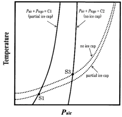
Fig. 5. A schematic illustration ofP–Tdiagram which appeared in McKay
et al.(1991). The dashed lines show an average temperature of Mars as a function of Pair with partial ice cap (the present condition) and with no ice cap. The solid lines represent regolith adsorption curves for
Pair+Prego=C1andC2(C1<C2). Each solid line has one intersection, that is, there are two steady state solutions irrespective of the parameter value.
AIR system.
4.2 Evolution of Martian climate
According to stellar evolution models, the solar luminos-ity has increased since the solar system was formed (e.g., Gough, 1981). Therefore the horizontal axis of Fig. 3 can be regarded as the time axis, and to trace the curve leftward from the present state (S1) should correspond to the Martian climate history tracing back to the past. Because the solar luminosity would have been lower in the past, the surface temperature would have been lower, much more CO2would
have condensed to expand the ice sheet, and the regolith would have adsorbed more CO2. Therefore, in this respect,
the atmospheric CO2pressure should have been lower in the
past. On the other hand, the Martian CO2atmosphere might
have decreased during the history by some removal processes (e.g., Melosh and Vickery, 1989; Brain and Jakosky, 1998; Luhmann et al., 1992; Pollack et al., 1987). If the Mar-tian climate was warm and wet in the past because of strong greenhouse effect of CO2, the amount of atmospheric CO2
should have been larger than that at present. Then the impli-cation for the amount of CO2to have decreased in the past
as noted above seems to contradict the past warm climate. This apparent contradiction results from the assumption for the total amount of CO2in the AIR system to have been
constant. When we consider the evolution of Martian cli-mate system, the total amount of CO2 within the system
should change. For example, if there existed liquid water, the atmospheric CO2 would be consumed through silicate
weathering followed by precipitation of carbonate minerals (Pollack et al., 1987). It is also suggested that the atmo-spheric CO2 has escaped owing to impact erosion of the
et al., 1992).
In order to consider the evolution of Martian climate sys-tem, we assume the following two extreme scenarios for the removal of CO2from the AIR system.
Case I: A large amount of CO2was removed from the
sys-tem in a very short period early in the Martian history, and CO2did not decrease after that event.
Case II: The amount of total CO2 in the system has
de-creased gradually during the history of Mars after the end of the heavy bombardment period.
In both cases, we assume that the early Martian climate was warm and wet because of greenhouse effect of CO2, and
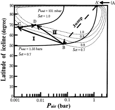
consider how the Martian climate evolves to the present con-dition. The hystereses of the steady state solution are shown in Fig. 6. For example, when Seff = 0.7 and Ptotal = 4
bars, there is one stable steady state solution “A”. This is the ice-free solution but liquid water can exist only in the equatorial region (the atmospheric CO2pressure is about 3.5
bars). Then, as some amount of CO2 was removed from
the AIR system due to impact erosion and/or weathering fol-lowed by carbonate precipitation, the total amount of CO2
would decrease. In this case, the time scale for decrease in CO2would be much shorter than that for increase in the solar
luminosity. The solution A would move along the curve left-ward with time, andfinally reach another solution A’where
Ptotal=1.35 bars. If the total amount of CO2decreases
fur-thermore, the Martian climate state should jump to the partial ice-covered solution“B”. This climate jump results in a dras-tic decrease in the atmospheric pressure and an expansion of the ice caps to the mid-latitude. Both the ice albedo and the
Fig. 6. The climate jump and the following two extreme scenarios for the evolution of the Martian surface environment. Case I: a large amount of CO2was removed from the system in a very short period early in the Martian history (A→A’→B→C), and then, the total CO2has been constant (C → D). Case II: after the end of the heavy bombardment period (A → A’ → B), the amount of total CO2 in the system has decreased gradually during the history of Mars (B→D). In both cases, climate jump (A’→B) should occur in its earliest history.
greenhouse feedbacks play significant roles in the climate jump: once ice caps were formed, the atmospheric pres-sure, so the greenhouse effect and the heat transport should decrease, but ice cap formation should increase the plane-tary albedo. Therefore, formation of the ice caps resulted in further cooling of the polar region. This climate jump is es-sentially the same as a“collapse”proposed by Haberleet al.
(1994). However, behaviors of the atmospheric CO2
pres-sure through and after the event are different: at the end of the climate jump (solution B), Pairis higher than that at present
in this model, although it is lower than that at present at the end of the collapse in the model of Haberleet al.(1994). This is because the model of Haberleet al.(1994) cannot express a change of the areal extent of polar ice caps although con-dition for the freezing point is quite different between at the pole and at the actual iceline. In this respect, our solution is different from that of Haberleet al.(1994). The steady state solution B is too cold for liquid water to exist. Thus, effec-tive decrease in the total CO2by precipitation of carbonate
minerals cannot occur hereafter.
In the Case I, the amount of the CO2atmosphere could have
decreased during short period compared with the timescale of solar luminosity change (B → C). Then, the solution may have approached the present state with an increase in the solar luminosity (C → D). It is noted that in Fig. 6 the atmospheric pressure at the point B (60 mbars) is much higher than that at the point C (∼1.5 mbars). This means not only that the greenhouse effect at the point B is stronger than that at the point C, but also that the freezing point at the point B is much higher than that at point C. In this case (evolution from the point B to the point C in Fig. 6), the effect of decrease in the freezing point exceeds the effect of decrease in the greenhouse effect. As a result, considering the pressure-temperature conditions at the ice line, the ice line retreats to the higher latitude while the CO2level (that
is, the global surface temperature) is lower at the point C than at the point B, even when the solar luminosity is constant. This is one of the most interesting results in this study. On the other hand, in the Case II, the amount of CO2decreased
on a timescale comparable to the solar luminosity change (B→D).
As mentioned above, Haberleet al.(1994) did not referred to either the B →C path or the B →D path, because Pair
must increase after the collapse in a scenario derived from their model. In both cases, if past Martian climate was warm and wet owing to the greenhouse effect of CO2, the climate
jump must have occurred during the evolution to the present state, and CO2ice caps on the early Mars could have extended
to the mid-latitude. It is noted that, even if the atmospheric CO2pressure decreases from the ice-free state, CO2ice caps
cannot be formed directly from that state whenSeffis larger
than 0.88 (see Fig. 2(a)). Therefore, if it were the case, the climate jump must have occurred before 1.6 Gyr (Seff=0.88)
(Gough, 1981). It might be consistent with the suggestion for the existence of the Austral ice sheet which might have extended to the mid-latitude of the southern hemisphere on Mars during the Hesperian age (Bakeret al., 1991).
It is noted that there must have been a supply of CO2
via volcanism, so the total amount of CO2may not have
argued that there is no solution of which the total amount of CO2have decreased throughout the Martian history to reach
the present condition. On the other hand, using the same model with Haberleet al.(1994), Gulicket al.(1997) sug-gested that pulses of CO2injected into the atmosphere more
recently than 4 Gyr can place the atmosphere into a stable, higher pressure, warmer state. At any rate, accurate evalu-ation of processes which control the amount of CO2 in the
AIR system should be required.
In this study, formation of H2O ice caps is not considered.
H2O ice caps might have affected the evolution of Mars from
warm and wet condition to cold condition. However, H2O ice
caps must have formed before the formation of CO2ice caps.
Thus, behaviors of CO2 ice caps can be discussed, at least
qualitatively, even if we do not consider formation of H2O
ice caps. However, if H2O ice caps exists, the temperature
in the polar region is lower than that with no H2O ice caps
owing to its high albedo. In such a case, CO2 ice caps are
formed under the higher solar constant than that predicted in this study.
4.3 Problem on CO2clouds
According to Kasting (1991), when CO2condensation is
included in the radiative-convective equilibrium model, the result differs remarkably from that of Pollacket al.(1987), especially forSeff=0.7 or 0.8. The greenhouse effect should
be reduced whenPairis above a few hundreds mbar because
of formation of CO2clouds, and what is worse, CO2
conden-sation limits the amount of atmospheric CO2. On the other
hand, Forget and Pierrehumbert (1997) showed that CO2ice
particle larger than 10μm can scatter infrared radiation back to the surface, thus CO2 clouds may have powerful
green-house effect. Because the effect of CO2clouds on the energy
balance may have been still unclear, the results shown here might be tentative. Therefore, we also consider the cases in which CO2cloud formation is included in the model (Fig. 7).
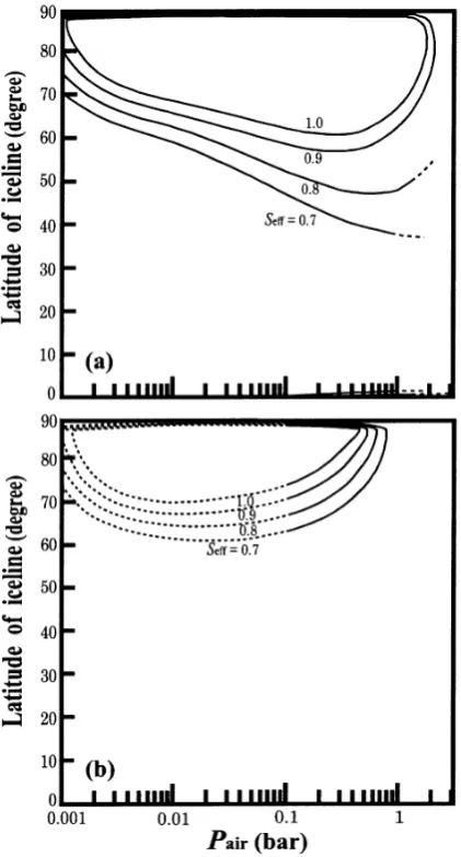
Figure 7(a) shows the solutions for the case which con-siders effects of CO2 cloud formation on the energy
bal-ance based on the results of Kasting (1991). In this case, an ice-free solution is impossible during the earliest history of Mars. For an initial state, a partial ice-covered solution (when
Ptotal≤3 bars) or ice-covered solution (whenPtotal>3 bars)
is expected. If the initial state was ice-covered, ice at the equatorial region should have disappeared during the evolu-tion asSeffincreased, and the steady state should have jumped
to a partial ice-covered state to reach the present condition. Figure 7(b) shows the solutions for the case based on the results of Forget and Pierrehumbert (1997) with radii of the CO2ice particles are 50μm, the optical depth is 10, and dry
atmosphere (note that they provided the results only above
Pair =100 mbar). As shown in thisfigure, area of the ice
caps at a certain Pairis smaller due to powerful greenhouse
effect of CO2 clouds. In this case, if the initial state was
ice-free, the solution cannot jump until Pairdecrease to, at
least, about 100 mbar, although we cannot know where the jump will occur because of absence of original data below 100 mbar.
It is expected that CO2cloud formation has been inhibited
in regions of atmospheric subsidence (Forget and Pierrehum-bert, 1997). Magnitude of the effect of CO2 clouds should
depend on fraction of cloud cover and optical thickness of
Fig. 7. Steady state solutions of the EBM based on the results of (a) Kasting (1991), and (b) Forget and Pierrehumbert (1997). Dashed curves represent the region where original data is not available.
the CO2cloud, but these properties have not been known. In
order to solve this problem, it is necessary to introduce a full 3-D climate model, but it is beyond the purpose of this study.
5.
Summary
In this paper, we have discussed the Martian surface envi-ronment. We assumed that CO2has been the dominant
con-stituent of the Martian atmosphere and that the atmosphere, the polar ice caps, and the regolith are major reservoirs of CO2
(the AIR system). In order to study stability and evolution of the AIR system, we introduced a one-dimensional energy balance climate model (EBM) which considers change of the ice cap area, latitudinal heat transport, and greenhouse effect of CO2.
point feedback is negative feedback which makes it stable. When we adopt the present state as a boundary condition and assume the total amount of CO2in the AIR system to be
con-stant, there exists two stable steady state solutions under the present solar luminosity. One corresponds to a partial ice-covered solution (the present state), and the other is a warmer ice-free solution. Although this seems to be consistent with the former results by Gierasch and Toon (1973) and McKay
et al.(1991), our result is different qualitatively from their results.
If the Martian climate was warm and wet owing to the greenhouse effect of CO2 in the past, the total amount of
CO2 contained in the system must have been much more
than that at present. This means that the total amount of CO2
in the system has been decreased by some removal processes. In this case, we found that the climate jump which is a drastic expansion of ice caps and decrease of the atmosphere must have occurred during the evolutionary path from the warm and wet condition to the present state, and ice caps on the early Mars could have extended to the mid-latitude. The atmospheric pressure may have decreased further after the climate jump.
Acknowledgments. The authors are most grateful to Y. Abe and T. Ikeda for helpful discussions and comments on this work. We also thank V. Gulick and an anonymous referee for the helpful reviews.
References
Baker, V. R., R. G. Storm, V. C. Gulick, J. S. Kargel, G. Komatsu, and V. S. Kale, Ancient oceans, ice sheets and the hydrological cycle on Mars,
Nature,352, 589–594, 1991.
Baker, V. R., M. H. Carr, V. C. Gulick, C. R. Williams, and M. S. Marley, Channels and valley networks, inMars, edited by H. H. Kiefferet al., pp. 493–522, Univ. of Ariz. Press, Tuscan, 1992.
Brain, D. A. and B. M. Jakosky, Atmospheric loss since the onset of the Martian geologic record: Combined role of impact erosion and sputtering,
J. Geophys. Res.,103, 22,689–22,694, 1998.
Budyko, M. I., The effect of solar radiation variations on the climate of the earth,Tellus,21, 611–619, 1969.
Fanale, F. P. and W. A. Cannon, Exchange of adsorbed H2O and CO2 be-tween the regolith and atmosphere of Mars caused by changes in surface insolation,J. Geophys. Res.,24, 3397–3402, 1974.
Fanale, F. P., J. R. Salvail, W. B. Banerdt, and R. S. Saunders, Mars: the regolith-atmosphere-cap system and climate change,Icarus,50, 381– 407, 1982.
Forget, F. and R. T. Pierrehumbert, Warming early Mars with carbon dioxide clouds that scatter infrared radiation,Science,278, 1273–1276, 1997. Gierasch, P. J. and O. B. Toon, Atmospheric pressure variation and the
climate of Mars,J. Geophys. Res.,30, 1502–1508, 1973.
Goldspiel, J. M. and S. W. Squyres, Ancient aqueous sedimentation on Mars,
Icarus,89, 392–410, 1991.
Gough, D. O., Solar interior structure and luminosity variations,Solar Phys.,
74, 21–34, 1981.
Gulick, V. C., D. Tyler, C. P. McKay, and R. M. Haberle, Episodic ocean-induced CO2greenhouse on Mars: implications forfluvial valley forma-tion,Icarus,130, 68–86, 1997.
Haberle, R. M., Early Mars climate models,J. Geophys. Res.,103, 28,467– 28,479, 1998.
Haberle, R. M., D. Tyler, C. P. McKay, and W. L. Davis, A model for the evolution of CO2on Mars,Icarus,109, 102–120, 1994.
Head, J. W., III, H. Hiesinger, M. A. Ivanov, M. A. Kreslavsky, S. Pratt, and B. J. Thomson, Possible ancient oceans on Mars: evidence from Mars Orbiter Laser Altimeter data,Science,286, 2134–2137, 1999. Hoffert, M. I., A. J. Callegari, C. T. Hsieh, and W. Ziegler, Liquid water
on Mars: an energy balance climate model for CO2/H2O atmosphere, Icarus,47, 112–129, 1981.
James, P. B., H. H. Kieffer, and D. A. Paige, The seasonal cycle of carbon dioxide on Mars, inMars, edited by H. H. Kiefferet al., pp. 934–968, Univ. of Ariz. Press, Tuscan, 1992.
Kasting, J. F., CO2condensation and the climate of early Mars,Icarus,94, 1–13, 1991.
Kasting, J. F., Warming early Earth and Mars,Science,276, 1213–1215, 1997.
Kieffer, H. H. and A. P. Zent, Quasi-periodic climate change on Mars, in
Mars, edited by H. H. Kiefferet al., pp. 1180–1218, Univ. of Ariz. Press, Tuscan, 1992.
Kuhn, W. R. and S. K. Atreya, Ammonia photolysis and the greenhouse effect in the primordial of the Earth,Icarus,37, 207–213, 1979. Leighton, R. B. and B. C. Murray, Behavior of carbon dioxide and other
volatiles on Mars,Science,153, 136–144, 1966.
Luhmann, J. G., R. E. Johnson, and M. H. G. Zhang, Evolutionary impact of sputtering of the Martian atmosphere by O+pickup ions,Geophys. Res. Lett.,19, 2151–2154, 1992.
McKay, C. P., O. B. Toon, and J. F. Kasting, Making Mars habitable,Nature,
352, 489–496, 1991.
Mellon, M. T., Limits on the CO2 content of the Martian polar deposits, Icarus,124, 268–279, 1996.
Melosh, H. J. and A. M. Vickery, Impact erosion of the primordial Martian atmosphere,Nature,338, 487–489, 1989.
North, G. R., R. F. Cahalan, and J. A. Coakley, Jr., Energy balance climate models,Reviews of Geophysics and Space Physics,19, 91–121, 1981. Pollack, J. B., J. F. Kasting, S. M. Richardson, and K. Poliakoff, The case
for a wet, warm climate on early Mars,Icarus,71, 203–224, 1987. Postawko, S. E. and W. R. Kuhn, Effect of the greenhouse gases (CO2,
H2O, SO2) on Martian paleoclimate,Proc. Lunar Planet. Sci. Conf. 16th, Part 2,J. Geophys. Res.,91, suppl., D431–D438, 1986.
Sagan, C. and C. Chyba, The early faint Sun paradox: Organic shielding of ultraviolet-labile greenhouse gases,Science,276, 1217–1221, 1997. Sagan, C. and G. Mullen, Earth and Mars: Evolution of atmospheres and
surface temperatures,Science,177, 52–56, 1972.
Smith, D. E., M. T. Zuber, H. V. Frey, J. B. Garvin, J. W. Head, D. O. Muhleman, G. H. Pettengill, R. J. Phillips, S. C. Solomon, H. J. Zwally, W. B. Banerdt, and T. C. Duxbury, Topography of the northern hemisphere of Mars from the Mars Orbiter Laser Altimeter,Science,279, 1686–1692, 1998.
Stone, P. H., A simplified radiative-dynamical model for the static stability of rotating atmospheres,J. Atmos. Sci.,29, 405–418, 1972.
Tanaka, H. M. and Y. Abe, A numerical study of the difference between the south and north CO2polar caps on Mars,Proc. Lunar Planet. Sci., XXIV, 1–7, 1991.
Toon, O. B., J. B. Pollack, W. Ward, J. A. Burns, and K. Bilski, The astro-nomical theory of climate change on Mars,Icarus,44, 552–607, 1980. Zent, A. P. and R. C. Quinn, Simultaneous adsorption of CO2and H2O
under Mars-like conditions and application to the evolution of the Martian climate,J. Geophys. Res.,100, 5341–5349, 1995.