F U L L P A P E R
Open Access
2.5D regularized inversion for the
interpretation of residual gravity data by a
dipping thin sheet: numerical examples and
case studies with an insight on sensitivity and
non-uniqueness
Salah A. Mehanee
*and Khalid S. Essa
Abstract
A new two-and-a-half dimensional (2.5D) regularized inversion scheme has been developed for the interpretation of residual gravity data by a dipping thin-sheet model. This scheme solves for the characteristic inverse parameters (depth to topz, dip angleθ, extension in depthL, strike length 2Y, and amplitude coefficientA) of a model in the space of logarithms of these parameters (log(z), log(θ), log(L), log(Y), and log(|A|)). The developed method has been successfully verified on synthetic examples without noise. The method is found stable and can estimate the inverse parameters of the buried target with acceptable accuracy when applied to data contaminated with various noise levels. However, some of the inverse parameters encountered some inaccuracy when the method was applied to synthetic data distorted by significant neighboring gravity effects/interferences. The validity of this method for practical applications has been successfully illustrated on two field examples with diverse geologic settings from mineral exploration. The estimated inverse parameters of the real data investigated are found to generally conform well with those yielded from drilling. The method is shown to be highly applicable for mineral prospecting and reconnaissance studies. It is capable of extracting the various characteristic inverse parameters that are of geologic and economic significance, and is of particular value in cases where the residual gravity data set is due to an isolated thin-sheet type buried target. The sensitivity analysis carried out on the Jacobian matrices of the field examples investigated here has shown that the parameter that can be determined with the superior accuracy isθ(as confirmed from drilling information). The parametersz,L,Y, andAcan be estimated with acceptable accuracy, especially the parametersz
andA. This inverse problem is non-unique. The non-uniqueness analysis and the tabulated inverse results presented here have shown that the parameters most affected by the non-uniqueness areLandY. It has also been shown that the new scheme developed here is advantageous in terms of computational efficiency, stability and convergence than the existing gravity data inversion schemes that solve for the characteristic inverse parameters of a sheet/dike.
Keywords: Regularized 2.5D residual gravity data inversion; 3D thin-sheet inversion; Log-space inversion; Non-uniqueness analysis; Convergence analysis; Sensitivity analysis
*Correspondence: [email protected]
Department of Geophysics, Faculty of Science, Cairo University, Giza, Egypt
Background
Gravity and magnetic methods have many successful applications in mineral prospecting, environmental appli-cations, and crustal imaging (e.g., Abdelrahman et al. 1989; Ateya and Takemoto 2002; Batista-Rodríguez et al. 2013; Beiki and Pedersen 2011; Fedi 2007; Hinze 1990; Hinze et al. 2013; LaFehr and Nabighian 2012; Long and Kaufmann 2013; Mehanee 2014a; Nettleton 1976; Okubo et al. 2013; Paoletti et al. 2013; Pei et al. 2014).
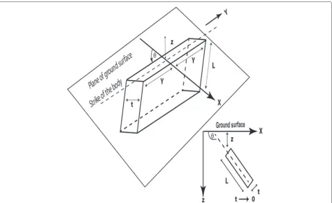
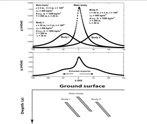
Techniques based on some geometrically simple bodies (e.g., sheet) have been in use for the analysis of mag-netic and gravity data acquired along profiles since the 1960s (e.g., Grant and West 1965). These techniques (e.g., Ateya and Takemoto 2002; Mushayandebvu et al. 2001; Sazhina and Grushinsky 1971) are applied to obtain the characteristic inverse parameters of the underlying target. Three-dimensional (3D) thin-sheet model is a very good approximation to a prismatic structure (e.g., an ore vein), unless the thickness is somewhat greater than the depth to the top (Telford and Geldart 1976) (Fig. 1). 3D thin-sheet models can be used to describe and resemble, for exam-ple, dikes or veins in exploration geophysics (Grant and West 1965; Pirajno and González-Álvarez 2013; Santosh and Pirajno 2014). Furthermore, thin-sheet solutions are favored for their inexpensive computational cost (Holstein et al. 2010) compared to full parallelepiped (e.g., Sazhina and Grushinsky 1971) and polyhedral (e.g., Holstein and Ketteridge 1996; Holstein 2003) solutions.
Inverse interpretation of an isolated residual gravity anomaly by a 3D thin-sheet model remains of interest in geophysical prospecting (e.g., Grant and West 1965; Telford et al. 1976). The main objective of the interpre-tation in this case is to retrieve the characteristic inverse parameters of the 3D approximative model: depth to the top, thickness, extension in depth, extension in the strike direction, and direction and amount of dip.
Grant and West (1965) described a graphical method for the interpretation of a residual gravity anomaly mea-sured along a profile by a 3D dipping thin-sheet model. The approach was successfully applied to sulfide prospect-ing. However, the drawback with this method is that it is based on sets of main and auxiliary characteristic curves, and it essentially demands interpolation between pairs of characteristic curves in order to estimate the magnitudes of the sheet parameters. Telford and Geldart (1976) pre-sented and described the forward modeling formula of 3D thin-sheet model, which is the basis for the inversion scheme developed here. They also highlighted the limita-tions (which are reported above) of this formula. Holstein et al. (2010) used the concept of gravi-magnetic sim-ilarity, and extended the thin-sheet potential modeling formula to include the potential, field, and field gradi-ent in both gravity and magnetic cases when the buried bodies have uniform density or magnetization. Holstein
and Anastasiades (2010) derived an exact finite expansion for the forward modeling computation of the gravita-tional anomaly of a uniform thin-polygonal sheet. This expansion exhibits the required absolute numerical sta-bility (Holstein and Anastasiades 2010). One can refer to Holstein and Ketteridge (1996) and Holstein et al. (2014), and the references therein, for a more detailed and com-prehensive information on this particular thin-polygonal sheet subject. Beiki and Pedersen (2011) developed a data window constrained two-dimensional (2D) inver-sion technique for the interpretation of gravity gradient tensor data using dike/sheet and contact models. By defi-nition, a data window contains a number of particular data points out of the entire measured gravity profile (Beiki and Pedersen 2011). These particular data points are mea-sured with respect to the center (that is located at the maximum response of the profile) of this window. This means that the gravity data points located to the left and right flanks of a window were not considered in the inversion. In other words, the full measured grav-ity signature (that is, primarily influenced by the buried anomalous structure) was not considered in the inter-pretation. A series of successive data windows is con-structed by increasing the number of data points used (out of the whole gravity profile) for estimating the target parameters (Beiki and Pedersen 2011). Beiki and Pedersen (2011) used the MATLAB nonlinear least squares opti-mization tool “lsqnonlin” to solve the miniopti-mization prob-lem of their scheme. This minimization tool is based on the Levenberg-Marquardt method (Levenberg 1944; Marquardt 1963). The convergence of the Levenberg-Marquardt method and its corresponding inverse param-eters (e.g., the depth, dip angle, and thickness of the buried target) obtained from each window were plotted in their paper. According to Beiki and Pedersen (2011), solution with the smallest data fit error is selected (out of the entire solutions retrieved from all attempted data windows) as the most reliable one. It appears from the numerical models analyzed by Beiki and Pedersen (2011) that the use of a few data points (out of the whole mea-sured gravity profile) in inversion was essential so that the Levenberg-Marquardt method can converge. Note that the aforementioned limitations (that are pertinent to the number of data points used in inversion and to the convergence and stability of the minimizer) are sat-isfactorily treated and fully well illustrated here as will be seen. Note that the Levenberg-Marquardt method (Madsen et al. 2004) was used also in the seismic tomog-raphy inversions.
Fig. 1A sketch showing geometry and characteristic parameters (depth to the topz, extension in depthL, finite extension in the strike direction 2Y, thicknesst, and direction and amount of dipθ) of a 3D dipping thin-sheet-like target (Grant and West 1965)
simulated a model described by a dike curvature and a density compaction.
From this review, it appears to us that Grant and West (1965) are the only authors to have developed a method for the quantitative inverse interpretation of a residual gravity profile measured over a 3D dipping structure by 3D dipping thin-sheet model. Consequently, to the best of our knowledge, a regularized scheme (based on 3D dip-ping thin-sheet type model) for the inversion of residual gravity anomaly measured along a profile over a 3D body was not developed before.
The objective of this paper is to develop an efficient and rigorous regularized inversion scheme (based on 3D dipping thin-sheet model) for the interpretation of a resid-ual gravity anomaly measured along a profile traversing the center of a 3D buried anomalous structure and nor-mal to the strike of this structure. This inversion scheme is called two-and-a-half dimensional (2.5D) inversion (see e.g., Hinze et al. 2013, p. 177). The developed scheme is capable of dealing with the nonlinearity and the ill-posedness of this 2.5D inverse problem and has many merits. First, it inverts the entire residual gravity data set rather than just a few characteristic points out of this data set. Second, it simultaneously recovers all the characteristic inverse parameters (depthz, direction and amount of dipθ, extension in depthL, strike length 2Y,
to the model parameters sensitivities in relation to non-uniqueness.
The paper is structured as follows. First, we briefly describe the direct problem (“Forward modeling solution” subsection). Second, the formulation of this particular inverse problem and its solving is discussed. Third, before applying this method to real data, the accuracy of the scheme is assessed and verified to numerical models with and without noise. Finally, the applicability of the developed technique to real data is demonstrated on two published field data examples from mineral exploration.
Methods
Forward modeling solution
The gravity anomaly(g), due to a 3D dipping thin-sheet target at a point x along a profile traversing the center of the target and normal to the target’s strike direction (Fig. 1), has a closed-form solution and is given (Grant and West 1965; Telford and Geldart 1976) by
g(xi,ρ,t,θ,z,Y,L)=2γ ρt
wherexiis the coordinate (m) of the measurement station, ρis the density contrast (kg.m−3),tis the thickness (m),
θ is the dip angle (degrees) of the body measured anti-clockwise,zis the depth (m) to the top, 2Y is the strike length (m),Lis the dipping extent (m) of the body, andγis the gravitational constant (6.67384×10⁻¹¹m3kg−1s−2). As indicated in the “Background” section, the thin sheet described above is a good approximation to a 3D pris-matic structure, unless the thickness is somewhat greater than the depth to the top (z) (Telford and Geldart 1976). The presence of the thickness (t) outside the main square bracket of formula (1) is a consequence of the thin-sheet assumption used in deriving this formula.
Note that formula (1) can be used to accurately simu-late a two-dimensional (2D) target by substituting in this formula a large value for the parameter Y (Grant and West 1965). Analysis of formula (1) with respect to the 2D simulation accuracy is beyond the scope of this paper.
It is noted that the parameters ρ andt can be com-bined into a single parameter (the so-called amplitude coefficient, A (kg.m−2) = ρ t) to help minimize the
non-uniqueness nature of this particular inverse prob-lem. Non-uniqueness means that many different models (approximative solutions) could fit the observed data with the same accuracy (e.g., Tarantola 1987). The matter per-tinent to the aforementioned parameter combination will be discussed further in the “Discussion” section.
Formulation of this 2.5D inverse problem and its solving
In this paper, we seek to solve the discrete 2.5D nonlinear inverse problem described by the operator equation (e.g. Menke 2012)
G(m)=g◦, (2)
whereGis the forward modeling operator acting onmto produce some predicted gravity data(g(x,A,z,Y,L, θ)) at a finite number (N) of observation points along a pro-file,mis a column vector of the model parameters (that is the vector of some approximative solution) we seek to retrieve from inversion (m =[A,z,Y,L,θ]T),g◦is a col-umn vector of a finite set of noisy gravity data measured along this profile,g◦=[g◦1,g◦2,g◦3,. . .g◦N]T, andTis the transposition operator.
Equivalently, Eq. 2 can be written as
g(xi,A,z,Y,L,θ)=g◦i, 1≤i≤N. (3)
Recent advances to solve the inverse problem of gravi-metric data are based on the use of deterministic approaches that utilize the regularized least squares tech-niques and the differentiability of the objective function subject to minimization (e.g., Zhdanov 2002). As indi-cated earlier, the inversion scheme described in this paper recovers the characteristic parameters of the buried target in a minimal time (a few seconds). Therefore, automatic deterministic approaches are much more efficient (see, for example, Mehanee 2015) than the approaches that are based on the trial-and-error modeling method.
Since the residual gravity data are usually corrupted with some noise, we do not seek to fit them exactly (Tarantola 2005). Rather, we seek (Ramlau 2005; Zhdanov 2002)
wheregis a column vector of the predicted data calculated along the profile, using formula (1), from some approx-imative solution m, g =[g1,g2,g3,. . .gN]T, andδ is the
noise level embedded in the measured data (go).
of the Tikhonov parametric functional (e.g., Mehanee and Zhdanov 2002; Tikhonov et al. 1998):
φ (m,g◦,α) = G(m) − g◦2 +
whereα(dimensionless) is the regularization parameter, the selection of which is addressed in the “Discussion” section, and Cz employed in (5) in order to adjust the inconsistency of units of the six terms ofφ (m,g◦,α)and in order to make the values of the C terms comparable (balanced). Given the aforementioned units of those constants,φ (m,g◦,α) in this case (that is, in this particular choice of units) is given in the units of mGal2. Equivalently, (5) can be readily re-written as:
The first term of (6) is the data misfit functional, deter-mined as the square norm of the difference between the observed and predicted data, and the second term is a stabilizing functional, the stabilizer.
The characteristic model parameters (A,z,Y,L, andθ) of a 3D thin sheet can have large variations in magni-tude (e.g.,z = 100 m,A = 105kg.m−2) which can mean
that the smaller parameters are ignored in the inversion as they have smaller sensitivities. Performing the inver-sion in the logarithmic space of the model parameters
(log(|A|), log(z), log(Y), log(L), and log(θ))makes these logarithmed parameters and their corresponding sensitiv-ities comparable and balanced as will be seen. In other words, the logarithmed variants will not dominate one another as do the non-logarithmed values. Furthermore, the inversion in the logarithmic space of the model param-eters forces and guarantees the positivity of the model parameters we seek. Inversion in the non-logarithmic (lin-ear) space (that is, the space of the model parameters themselves:A,z,Y,L, andθ) can generate negative model parameters, and hence results in scheme divergence (e.g., Mehanee 2014a). Therefore, the new logarithmed-space objective functional takes the form:
(m,g◦,α)=τ G(m) − g◦2+α m2=min, (7)
whereτ is a scaling parameter used in order to make dimensionless and is set to 1
scaling parameters) is of a unit (positive) value and is introduced in order to make the quantities that are under the logs in mdimensionless. The introduction of these parameters is physically necessary because the logs do not allow dimensions to be defined. As mentioned above,
α is a dimensionless quantity. Note that hereinafter the scaling parameters of m are dropped to simplify the notations.
All the numerical models and real data examples shown here are inverted and analyzed by the logarithmic min-imization formulation presented in (7). We note that, in the restricted case of the noise-free and neighbor-ing/interference effect-free numerical example (Model 1), the nonlinear minimization problem (7) is solved itera-tively using a sequential hybrid technique that automat-ically combines the SD and GN methods (see Mehanee 2015, and the references therein) in order to verify and val-idate the developed inversion scheme prior to applying it to noisy and real data sets.
The use of the hybrid technique was essential. This is because theSDmethod converges very slowly or stagnates (as found from extensive noise-free numerical experi-ments) at the final stage of its iterative minimization process. It was also found from these experiments that the
GN method essentially requires a very good initial guess in order to converge (Zhdanov 2002). That is why the SD method (which does not require a good initial guess to converge as will be seen in the “Numerical tests” subsec-tion) is employed first in the developed scheme in order to generate and prepare a suitable initial guess for theGN
method.
In the framework of this hybrid scheme, the SD method is used first until a normalized misfit (defined as
G(m)−g◦
g◦ ×100 %) of roughly around 5−10 % (depending on the model subject to inversion) is reached. After that, the GN method is applied to the observed data, where the inverse results produced from the SD method is used as the initial guess for the GN method. The GN method terminates when a normalized misfit below 10−5 % is reached.
field data), we neither expect nor seek to exactly fit the observed data (see the figures pertinent to Model 2 and Model 3).
The entire computational steps of the GN and SD meth-ods of the inverse scheme are presented and discussed in Appendices 1 and 2. The code of the scheme is imple-mented in MATLAB. We note that no built-in MATLAB optimization (minimization) functions were used in the 2.5D code of our paper.
Sensitivity (Fréchet) matrix calculation
The Jacobian (Fréchet) matrix (F) used in this scheme is calculated analytically with respect to the inverse param-eters we seek(log(|A|), log(z), log(Y), log(L), and log(θ))
The use of the logarithmed model parameters has the benefit of making the aforementioned derivatives dimen-sionally the same, which is a good strategy for balancing the Jacobian terms. The quantities ∂∂Ag, ∂∂gL, ∂∂gz, ∂∂θg, and∂∂Yg are evaluated analytically by differentiating the forward modeling formula (1).
Singular value decomposition
The singular value decomposition (SVD) of an m × n
matrix (in our case this matrix isFRN×5, whereNand 5, respectively, are the number of data points along the grav-ity profile and model parameters) is given (e.g., Jupp and Vozoff 1975) by:
F=U S VT, (9)
whereU =[u1,u2,. . .,um] Rm×mandV =[v1,v2,. . ., vn] Rn×n are both orthogonal matrices.S Rm×n is
a diagonal matrix with non-negative real values (the so-called singular values) arranged in decreasing order,s1 ≥ s2. . . . ≥ sn ≥ 0. The sequence S =[s1,s2,. . .,sn] is
referred to as the singular spectrum ofF. The columns of U =[u1,u2,. . .,um] and V =[v1,v2,. . .,vn] are the
left and right singular vectors in the input and output spaces of the transformation represented by F, respec-tively. The magnitude of the singular values inSrepresents
and determines the corresponding important singular vectors in the columns of U andV. The SVD is a use-ful tool for understanding the sensitivity analysis of the various model parameters of the 3D thin-sheet model as will be seen.
Results and discussion Numerical tests
Prior to applying the developed inversion algorithm to real data examples, its accuracy is assessed and analyzed first on three numerical models. All inverse solutions are rounded to the first integer.
Model 1: noise-free example
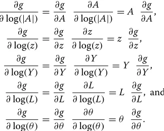
The gravity response of a thin-sheet type model withz=
25 m,L=50 m,Y=500 m,θ =30o, andA=5700 kg/m2 is generated at the ground surface (Fig. 2).
The presented algorithm supplemented with the SD method was applied to this noise-free dataset for 6000 iterations (yielding to a normalized misfit of about 4.7 %) using the initial guess shown at the top panel of Fig. 2. The corresponding inversion results (the so-called the preliminary inverse solution) are shown at the top panel of Fig. 2. To avoid possible stagnation with the SD method, the same algorithm supplemented with the GN method was applied to the same residual gravity data. The aforementioned preliminary inverse solution evolved from the SD method was employed automatically, as initial guess, in the GN method. The bottom panel of Fig. 2 shows the final inverse solution obtained from the scheme.
It is seen that the algorithm has converged below 10−6% (normalized misfit) and successfully recovered the true value of all inverse parameters of the buried body. Note that the observed data and predicted response are coin-cident with each other. The regularization parameter (α) used in the SD and GN methods is 10−5 and 10−12,
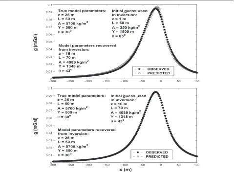
respectively. Figure 3 depicts the behavior of the misfit and objective functional corresponding to the SD and GN inversion results shown in Fig. 2.
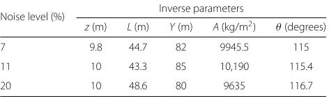
Model 2: noisy example
In order to assess and analyze the robustness and stability of the inverse algorithm, the developed scheme has been applied to a noisy profile. Subsequent noise levels of about 7, 11, and 20 % have corrupted the gravity data generated by a numerical model described by the following:z=12 m,L=35 m,Y=100 m,θ =120◦, andA=12,000 kg/m2. Each noise level was separately generated and added to the noise-free data setG(m)using the MATLAB function “awgn” in order to produce the corresponding corrupted data setg◦subject to inversion. The aforementioned noise
levels were separately calculated as g◦−gG(m)
Fig. 2Model 1: noise-free data.Top panel: preliminary (initial) inversion results obtained from the steepest descent (SD) method.Bottom panel: final inversion results obtained from the Gauss-Newton (GN) method which used the inversion results produced from the SD (top panel) as initial guess; see the text for details.Bottom panelshows that the observed and predicted data are coincident with each other
The corresponding final inversion results produced by the SD method are rendered in Fig. 4. The scheme ter-minated when the embedded noise level is reached by the SD method. Figure 5 shows the behavior of the mis-fit and objective functional corresponding to the inversion results shown in Fig. 4. Anαof 10−6was used in all the inverse calculations of this model.
The obtained inversion results show that the developed inverse technique is stable with respect to the noise lev-els embedded. Tables 1 and 2 present the inverse solutions and the corresponding error (in percentage) of each model parameter measured with respect to the true value of this parameter. One can see that error range of about 4–39 % was encountered in the retrieved inverse solutions. It can be seen that the highest errors are associated with the data set contaminated with the highest noise level (20 %), which is not unexpected. Note that the model parameter
θ encountered the smallest error in the case of the 20 % noise. Whereas the rest of the model parameters encoun-tered the smallest error in the case of the 11 % noise. This
could be attributed to the variation in the model param-eter sensitivities and noise level that contaminated the data.
Model 3: interference effect example
Fig. 3Model 1: noise-free data. Behavior of the misfit and objective functional corresponding to the SD (top panels) and GN (bottom panels) inversion results shown in Fig. 2
present in the middle of the profile and the two minor anomalies surrounding the prominent one.
Two interpretive scenarios are explored and investigated for analyzing and inverting the profile of the composite effect (Fig. 6, middle panel) by a single thin sheet (the subject of this paper). Scenario 1 (whole profile inver-sion) in which the whole profile is inverted and analyzed. Scenario 2 (extracted (truncated) profile inversion) in which only the distorted prominent anomaly (marked by arrows in Fig. 6, middle panel) out of the whole profile is inverted. Scenario 2, in this particular case, is probably more realistic (in terms of inverting its data by a single thin-sheet model) as its gravity response can resemble a single thin-sheet model. Scenario 1 is not so realis-tic (in terms of inverting its data by a single thin-sheet model) as its gravity response subject to inversion has three anomalous signatures that cannot be attributed to or represented by a single thin-sheet model. However, the
inversion of scenario 1 has been carried out here solely for the sake of investigative purpose, better understand-ing and for the full illustration of the developed inversion scheme.
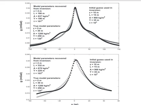
The top panel of Fig. 7 shows the true model parameters of the main body and the corresponding approximative inverse results of Scenario 1 for which a normalized misfit of about 10.85 % is reached using an
α of 10−6. The inversion results of Scenario 2 are shown
in the bottom panel of Fig. 7. A normalized misfit of 6.71 % is obtained, and an α of 10−9 was used in the
inverse computations. This analysis shows that the param-eters A,L, andY of the main body exhibited significant inaccuracy.
Fig. 4Model 2: noisy data. Inversion results corresponding to various noise levels. Data corrupted with about 7 % (top panel), 11 % (middle panel), and 20 % (bottom panel) noise. The results shown in this figure and all subsequent figures are recovered by the SD method solely . See the text for details
neighboring/interference effect. Isolated targets (such as ore veins and dikes) are frequent in many geologic set-tings and can be of a paramount economic interest as will
Fig. 5Model 2: noisy data. Behavior of the misfit and objective functional corresponding to the inversion results shown in Fig. 4. The top, middle and bottom panels correspond to those of Fig. 4
Field data inversion
In order to examine and assess the applicability of the developed inversion technique, two published field examples, from mineral exploration in Canada and Cuba, with various depth of burial, geologic complexity, and interference effects are analyzed. These particular data sets were selected in this research paper for a number of
Table 1Model 2 (noisy data). Inversion results of various noise
levels. The true model parameters arez=12 m,L=35 m,Y=
100 m,A=12,000 kg/m2, andθ=120 °
Noise level (%) Inverse parameters
z(m) L(m) Y(m) A(kg/m2) θ(degrees)
7 9.8 44.7 82 9945.5 115
11 10 43.3 85 10,190 115.4
20 10 48.6 80 9635 116.7
reasons. First, these data sets were generated by buried causative ore bodies, which can resemble thin-sheet models (Davis et al. 1957; Grant and West 1965; Siegel et al. 1957), the subject of this paper. Second, these data sets were measured from sites with known drilling infor-mation; hence, we can compare the numerical results yielded from the inversion against those confirmed from drilling. Third, these sites have core samples from
Table 2Model 2 (noisy data). Error of the inversion results shown in Table 1
Noise level (%) Error of inverse parameters (%)
z L Y A θ
7 18.3 27.7 18 17 4.2
11 16.6 23.7 15 15 3.8
which the density contrasts were accurately estimated in laboratory. As pointed out earlier, the knowledge of the density contrast (ρ) is essential in order to compute the thickness (t) of the body from the amplitude coefficient (A) obtained from the inversion.
The Mobrun anomaly, Canada
Inverse resultsA prominent Bouguer gravity anomaly was observed over a massive sulfide ore body in the Noranda Mining District, Quebec, Canada (Grant and West 1965; Siegel et al. 1957). Figure 8 shows the SW-NE residual gravity profile (whose location is shown in Figure 10-1, page 272, Grant and West 1965) taken normal to the strike of the buried causative ore vein. Directional drilling inter-sected sulfides over a distance slightly greater than 30.5 m
(Grant and West 1965, page 282, see also Figure 10-11 in page 281).
Grant and West (1965) reported that the average den-sity of core samples of the mineral taken from drilling was 4600±500 kg/m3, and for the host rock, the density was
about 2700 kg/m3. Hence, the ore body has a density con-trast (ρ) of 1400–2400 kg/m3. Thus, the aforementioned two density values are equal to the bulk densities of the ore and the host rock, respectively.
The inverse algorithm has been applied to the above mentioned residual gravity profile. Figure 8 shows the two approximative inverse solution sets obtained from two dif-ferent regularization parameters (α) using an initial guess of (z=2 m,L=30 m,A=2200 kg/m2,Y =50 m, and
θ = 30°). The inversion results shown at the top panel
Fig. 7Model 3: neighboring/interference effect of three nearby bodies.Top panel: approximative inverse solution obtained from the inversion of the whole profile shown in the middle panel of Fig. 6.Bottom panel: approximative inverse solution obtained from the inversion of the extracted (truncated) response (marked byarrowsin the middle panel of Fig. 6). See the text for details
were recovered using anα of 10−7and correspond to a normalized misfit of 2.93 %. The bottom panel illustrates the results retrieved from the algorithm using an α of 10−4, for which a normalized misfit of 2.48 % was reached. It is noted that the density contrast range mentioned above was used to estimate the corresponding thickness (t) range of the ore body from the amplitude coefficient (A=tρ) evolved from the inversion.
In order to monitor and assess the non-uniqueness (equivalence) issue, which is not unexpected for this par-ticular inverse problem, several initial guesses were also attempted in the scheme. Table 3 summarizes all obtained inversion results. It can be seen from the table that the regularization parameter indeed can affect the inverse solutions.
One can see that the two approximative solution sets (the so-called here “Equivalent Model 1” and “Equivalent Model 2”) shown at rows 3 and 5 of Table 3 are different, though each of them has the same normalized misfit value
(2.7 %). This is attributed to the non-uniqueness nature of this particular inverse problem; that is, different inverse models can equally fit the observed data.
On the basis of thea prioriinformation (which includes the contour form of the residual gravity map from which the gravity profile subject to inversion was taken), it can be suggested that the approximative inverse solutions pre-sented in rows 4, 5, and 6 of Table 3 are not very realistic. On the other hand, these tabulated results suggest that the most common model (interpretive model to resemble the buried vein deposit) could be that shown in rows 1, 2, and 3. In light of this, it is reasonable to suggest that the cor-responding inverse parameters of the interpretive model can be the averages of those shown in the aforementioned three rows. Therefore, the interpretive model is described by z =12.4 m, L= 184.4 m,A= 55,791.2 kg/m2, Y =
Fig. 8The Mobrun anomaly, Canada. Inversion results obtained from two different regularization parameters(α)and same initial guess. The results shown at thetopandbottompanels correspond to a normalized misfit of 2.93 and 2.48 %, respectively. The measured and predicted data are shown insolidandopen circles, respectively
model suggested here. The results confirmed from drilling (z, t, and Y), and those recovered from inversion are in reasonable match. We note that other gravity inversion methods (e.g., Li and Oldenburg 1998; Zhdanov et al. 2004) could produce a better fit.
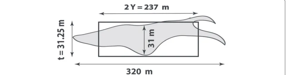
The parameterAretrieved from inversion (A=55,791.2 kg/m2) suggests a thickness of 23–40 m (t= 23–40 m) which is greater than the depth recovered from inversion (z = 12.4 m). Probably this is because the actual ore
body is not a thin sheet. Supporting evidence is that the actual ore body has a thickness of 31 m as revealed from a slice (constructed from drilling) taken at 50 m depth (Fig. 9). And that the depth to the top of the target is less than 30.5 m as inferred from directional drilling that inter-sected the body at about 30.5 m. As pointed out in the “Forward modeling solution” subsection, the 3D thin sheet is a good approximation to a prismatic structure, unless the thickness (t) is somewhat greater than the depth
Table 3The Mobrun anomaly, Canada. Tabulated inversion results.αis the regularization parameter
Misfit % α Initial guess Inverse solution
z(m) L(m) Y(m) A(kg/m2) θ(degrees) z(m) L(m) Y(m) A(kg/m2) θ(degrees)
2.93 10−7 2 30 50 2200 30 11 203 125 52,604 86
2.48 10−4 2 30 50 2200 30 14 172 113 58,801 86
2.7 10−2 10 500 500 2000 120 12 178 118 55,968 86
2.47 10−4 10 500 500 2000 120 14 119 262 59,631 86
2.7 10−4 10 1000 80 20,000 10 17 299 55 75,420 86
Fig. 9The Mobrun anomaly, Canada. Plan showing the Mobrun sulfide ore body (ingray), outlined from drilling, at 50 m depth (from Grant and West 1965). The inversion results are marked by theblack box
to the top (z) (Telford et al. 1976). However, we sought in this paper to fit and interpret this residual gravity profile by a thin-sheet-like model for investigative purposes and the full illustration of the developed inverse scheme, and in order to gain some insights.
Prior to any drilling in this area, Siegel et al. (1957) ana-lyzed this gravity profile based on a 2D trial and error modeling method and reported a corresponding solution of z = 6 m,L = 186 m, and t = 31 m. It is relevant to note that the strike length of the deposit in this case is assumed to be infinite as the interpretation was essen-tially based on 2D assumption. Grant and West (1965) too interpreted this profile but as a 3D thin sheet, based on a graphical method, and the retrieved inverse solu-tion is as follows: z = 17 m, L = 170 m, 2Y (strike length)=205 m,θ = 83◦, andt = 36 m. These results, too, show that the approximative model is quasi-vertical. Using an Euler deconvolution technique, Roy et al. (2000) interpreted this profile by a 2D vertical ribbon model and obtained an inverse model ofz= 22.7 m andL=52 m. While their results are in some variations from the true results confirmed from drilling, these results are still use-ful as they could be used as a reasonable initial guess in deterministic (gradient-type) inversions. As noted above, other gravity inversion methods (e.g., Li and Oldenburg 1998; Zhdanov et al. 2004) could produce a more accurate inverse solution and fitting.
Sensitivity analysis
In order to get some insights on a possible mutual inter-relation between the non-uniqueness of this particular inverse problem and the model parameter sensitivities (that is, the Fréchet matrix;F = ∂∂mg), the sensitivities of the aforementioned two equivalent solutions (“Equivalent Model 1” and “Equivalent Model 2”) and of the two ini-tial guesses used in the inversion of these two equivalent solutions have been calculated.
The top panel of Fig. 10 depicts the sensitivities (abso-lute values) computed from the initial guess (shown at row 3 of Table 3) from which “Equivalent Model 1” was
evolved. The sensitivities (absolute values, too) of the inverse parameters of “Equivalent Model 1” (shown, too, at row 3 of Table 3) are illustrated in the bottom panel of Fig. 10. The corresponding sensitivities of “Equivalent Model 2” and its initial guess (both are shown at row 5 of Table 3) are rendered in Fig. 11.
Note that the sensitivities of the inverse parameters log(L) and log(Y)(the two main parameters that appear to be most affected by the non-uniqueness of this par-ticular inverse problem as will be strengthened further and seen in the sensitivity subsection of the field exam-ple of the Camaguey area, Cuba) of “Equivalent Model 1” and “Equivalent Model 2” are found to be posi-tive real numbers. The bottom panel (corresponding to these two equivalent models) of Figs. 10 and 11 quali-tatively reveals that the sensitivity curves of these two parameters (log(L) and log(Y)) have a similar behavior and form. The degree of conformity of these two sen-sitivity curves depends upon the values of the model parameters used in the sensitivity calculation. The top and bottom panels of Figs. 10 and 11 show that the parameter log(θ)has the dominant sensitivity. Pertinent quantitative analysis based on the singular value decom-position (e.g., Press et al. 1988) is provided in the next paragraph.
In order to understand better the mutual interrelation between the non-uniqueness of this particular inverse problem and the model parameters sensitivity, the SVD (e.g., Jupp and Vozoff 1975, Press et al. 1988) was carried out separately on the Fréchet matrix of “Equivalent Model 1” and of the initial guess of this equivalent model.
Fig. 10The Mobrun anomaly, Canada. Sensitivity pertinent to this profile’s “Equivalent Model 1” and its initial guess (both are shown at row 3 of Table 3), see the text for details.Top panel: sensitivities calculated from the initial guess.Bottom panel: sensitivities calculated from “Equivalent Model 1”
Note that the first three singular vectors in the parame-ter space collectively achieved a variability of more than 99.9 % (Table 4). Figure 12 depicts the various compo-nents of the three aforementioned singular vectors. The left top panel (in which the components corresponding to the first singular value (s1 = 19.7) are plotted in linear
scale) shows that the parameter log(θ)has the most dom-inant effect. The right top panel (in which the absolute value of the same aforementioned components are plot-ted in log scale) shows that the order of the importance of parameters (for this particular model parameter set) is as follows: log(θ), log(|A|), log(L), log(Y), and log(z). This panel shows that the components pertinent to the parameters log(L)and log(Y)nearly have the same mag-nitude, this agrees well with the sensitivity curves (of these
two parameters) rendered at the top panel of Fig. 10 as the first right singular vector has the most variability as indicated above (97.73 %). Furthermore, the middle and bottom panels (pertinent to the second and third right sin-gular vectors, which collectively achieved a variability of 2.18 %) of Fig. 12 also show that the components pertinent to the parameters log(L) and log(Y) have a comparable magnitude.
Fig. 11The Mobrun anomaly, Canada. Sensitivity pertinent to this profile’s “Equivalent Model 2” and its initial guess (both are shown at row 5 of Table 3), see the text for details.Top panel: sensitivities calculated from the initial guess.Bottom panel: sensitivities calculated from “Equivalent Model 2”
log(θ)has the most dominant effect. This agrees with that revealed from the top left panel of Fig. 12. The top right panel of Fig. 13 shows that the order of the importance of parameters this time (that is, for “Equivalent Model 1”) is as follows: log(θ), log(L), log(Y), log(|A|), and log(z).
Table 4The Mobrun anomaly, Canada. Singular values and their variabilities in percentage of the sensitivity matrix, which was calculated from the initial guess shown at the top panel of Fig. 10
Singular values Variability in percentage
19.7 97.73
0.394 1.96
0.044 0.22
0.0171 0.085
0.0019 0.0094
This panel shows that the components pertinent to the parameters log(L), log(Y), and log(|A|)have a compara-ble magnitude, which conforms with the sensitivity curves (of these three parameters) shown at the bottom panel of Fig. 10. Furthermore, the middle and bottom panels of Fig. 13 also reveal that the components pertinent to the parameters log(L) and log(Y) have nearly a similar magnitude.
The Camaguey Province anomaly, Cuba
Inverse results
Fig. 12The Mobrun anomaly, Canada. Parameter eigenvectors corresponding to the first three singular values (denoted bys) (see the text for details) calculated from the singular value decomposition (SVD) analysis carried out on the Frechet matrix of the initial guess shown at the top panel´ of Fig. 10.Left panels: parameter eigenvectors in linear scale.Right panels: parameter eigenvectors’ absolute values in log scale
profile is taken normal to the strike of the residual gravity anomaly shown in the middle part of Fig. 6 of Davis et al. (1957).
This gravity profile is associated with the largest chromite deposit found in the province (Davis et al. 1957).
Table 5The Mobrun anomaly, Canada. Singular values and their variabilities in percentage of the sensitivity matrix, which was obtained from “Equivalent Model 1” shown at the bottom panel of Fig. 10
Singular values Variability in percentage
244.78 96.76
6.78 2.68
1.06 0.42
0.33 0.13
0.03 0.013
This prominent profile has a trend of S60oW to N60oE and overlies a chromite ore body which contains about 115,000 tons, dips steeply to the southwest, and comes within 3 m of the ground surface (Davis et al. 1957).
We have run the inversion using a number of various initial guesses to see the most common inverse solution. The top, middle, and bottom panels (which have identi-cal observed data and point curves) of Fig. 14 show the three approximative solution sets yielded from three dif-ferent initial guesses. A normalized misfit of about 7.56 % was reached in all cases. Set 1 has a solution ofz= 5.5 m,L=40 m,A=6989 kg/m2, 2Y(strike length)=60 m,
Fig. 13The Mobrun anomaly, Canada. Parameter eigenvectors corresponding to the first three singular values (see the text for details) calculated from the SVD of the Fr´echet matrix of “Equivalent Model 1” presented at the bottom panel of Fig. 10.Left panels: parameter eigenvectors in linear scale.Right panels: parameter eigenvectors’ absolute values in log scale
is seen that the approximative solutions of the parameters
L andY of Set 1 and Set 2 are nearly swapped. This is readily attributed to the non-uniqueness nature (solution equivalence) of this inverse problem—these two solutions (Set 1 and Set 2) are so-called here “Equivalent Model 1” and “Equivalent Model 2”. It appears that the com-mon solution is the one that is shown in Set 2 and Set 3. The depth shown in all sets is in a reasonable agreement with that obtained from drilling. Table 6 summarizes all inversion results.
The top panel of Fig. 15 illustrates the sensitivities (abso-lute values) calculated from the initial guess (shown at the top panel of Fig. 14) from which “Equivalent Model 1” was produced. The sensitivities (absolute values, too) of the inverse parameters of “Equivalent Model 1” (shown
too at the top panel of Fig. 14) are illustrated in the bot-tom panel of Fig. 15. The corresponding sensitivities of “Equivalent Model 2”, and its initial guess (both are shown at the middle panel of Fig. 14) are rendered in Fig. 16.
The sensitivity of the inverse parameters log(L), log(Y), and log(|A|) of “Equivalent Model 1” and “Equivalent Model 2” are found positive real number for this profile. The bottom panels of Figs. 15 and 16 show that these three parameters have quasi-similar behavior and form— this is consistent with the pertinent findings reported for the Mobrun anomaly, Canada (see the bottom panels of Figs. 10 and 11).
Sensitivity analysis
Fig. 14The Camaguey Province anomaly, Cuba. Residual gravity anomaly (redrawn from Figure 6 of Davis et al. 1957): inversion results retrieved from three various initial guesses
top panel of Fig. 15. This table shows that most of the variability (79.1 %) is captured by the first right singu-lar vector. Figure 17 illustrates the various components of the first three singular vectors. The top left panel shows that the parameter log(θ)has the most dominant effect as was observed, too, in “The Mobrun anomaly, Canada”
subsection. The top right panel shows that the order of the importance of parameters (for this particular model parameter set) is as follows: log(θ), log(|A|), log(z), log(L), and log(Y). This panel as well as the middle and bottom panels show that the components of all parameters have diverse magnitudes.
Table 6The Camaguey Province anomaly, Cuba. Tabulated inversion results
Misfit % α Initial guess Inverse solution
z(m) L(m) Y(m) A(kg/m2) θ(degrees) z(m) L(m) Y(m) A(kg/m2) θ(degrees)
7.56 10−4 100 200 300 20,000 30 6 40 30 6990 94
7.56 10−6 50 350 300 10,000 120 6 30 42 7647 94
Fig. 15The Camaguey Province anomaly, Cuba. Sensitivity pertinent to this profile’s “Equivalent Model 1” and its initial guess (both are shown at the top panel of Fig. 14), see the text for more details.Top panel: sensitivities calculated from the initial guess.Bottom panel: sensitivities calculated from “Equivalent Model 1”
Table 8 shows the singular values and their vari-abilities of the sensitivity matrix shown at the bottom panel of Fig. 15. This table shows that most of the variability (96.9 %) is held by the first right singu-lar vector. Figure 18 illustrates the various components of the first three singular vectors. The top left panel shows that the parameter log(θ) has the most domi-nant effect as was observed earlier. The top right panel shows that the order of the importance of parame-ters (for this particular model parameter set) is as fol-lows: log(θ), log(|A|), log(L), log(Y), and log(z). This panel and the middle and bottom panels show that the components of all parameters have comparable magnitudes.
The SVD analysis presented herein revealed that the parameter log(θ) has the highest importance in this
inverse scheme. All field examples, carefully analyzed here, have shown that the parameterθis determined very accurately (based on drilling information), and that this parameter is the least affected by the initial guess selec-tion and the misfit stopping criteria. It is worthy to note that accurate determination of the amount and direction of dip (θ) of the buried target can be of a paramount importance for effective decision making on directional drilling.
Fig. 16The Camaguey Province anomaly, Cuba. Sensitivity pertinent to this profile’s “Equivalent Model 2” and its initial guess (both are shown at the middle panel of Fig. 14), see the text for more details.Top panel: sensitivities calculated from the initial guess.Bottom panel: sensitivities calculated from “Equivalent Model 2”
Discussion
Gravity inversions based on regular models remain of interest in exploration geophysics (see for example, Biswas 2015, and the references therein). It is worthy to note that it is very rare to find a geologic target that is truly
Table 7The Camaguey Province anomaly, Cuba. Singular values and their variabilities in percentage of the sensitivity matrix, which was calculated from the initial guess shown at the top panel of Fig. 15
Singular values Variability in percentage
8.22 79.1
2.12 20.4
0.049 0.47
0.0006 0.0055
0.0002 0.0020
regular body. Nevertheless, these regular models often yield a first approximation solution, which is sometimes quite adequate (e.g., Abdelrahman et al. 1989; Mehanee 2014a).
Fig. 17The Camaguey Province anomaly, Cuba. Parameter eigenvectors corresponding to the first three singular values (denoted bys) (see the text for details) calculated from the SVD analysis carried out on the Fréchet matrix of the initial guess shown at the top panel of Fig. 15.Left panels: parameter eigenvectors in linear scale.Right panels: parameter eigenvectors’ absolute values in log scale
1. For reconnaissance analysis and pilot studies (for first approximative interpretation) in geophysical
prospecting prior to conducting large-scale gravity data surveys,
2. For comparative and ambiguity studies and joint
Table 8The Camaguey Province anomaly, Cuba. Singular values and their variabilities in percentage of the sensitivity matrix, which was calculated from “Equivalent Model 1” shown at the bottom panel of Fig. 15
Singular values Variability in percentage
33.66 96.88
0.861 2.48
0.18 0.52
0.038 0.111
0.0033 0.009
(e.g., gravity and magnetic data) inversion in order to minimize the non-uniqueness that is imperative here, and
3. For integrated and unequivocal interpretation. For example, this scheme can determine the amount and direction of dip of the buried target with greatest accuracy (as seen in the investigated inversions of the noisy numerical data and the field examples), which was confirmed by the sensitivity analysis carried out in our paper.
Fig. 18The Camaguey Province anomaly, Cuba. Parameter eigenvectors corresponding to the first three singular values (see the text for details) calculated from the SVD of the Frechet matrix of “Equivalent Model 1” presented at the bottom panel of Fig. 15.´ Left panels: parameter eigenvectors in linear scale.Right panels: parameter eigenvectors’ absolute values in log scale
rigorous 3D gravity inverse schemes. It is emphasized that we are not claiming that inversion schemes based on geo-metrically simple bodies replace the rigorous 3D gravity inverse schemes.
Rigorous 3D gravity inversion schemes (e.g., Li and Oldenburg 1998; Zhdanov et al. 2004) can simultaneously invert for several anomalous irregular bodies and nor-mally require areal data coverage. However, these schemes take much longer computation time (than the thin-sheet schemes) in order to yield the approximative inverse solu-tion (that is also non-unique), which comprises the 3D anomalous density distribution (ρ) in the subsurface. As indicated above, a reasonable initial guess is a prereq-uisite in the rigorous 3D gravity inverse schemes. These rigorous 3D schemes can generate smooth or focused (compact) inverse images (depending primarily upon the particular objective of the interpretation) by incorporat-ing the appropriate type of the stabilizer in the objective
functional subject to minimization. It is relevant to note that the inversion of focused (compact) images requires accurate information about the lower and upper bounds of the anomalous density distribution (ρ) of the buried targets.
Upon the completion of the gravity data acquisition and processing for an area, the following interpretation steps (e.g., Grant and West 1965; Hinze et al. 2013) are applied in order to estimate the characteristic parameters of a buried target:
developed here using several initial guesses. This will give first approximate interpretation about the underly-ing body. The value of the parameterθ(which determines the amount and direction of dip of the buried body) will be the most accurate (see column 12 of Tables 3 and 6) as confirmed from the numerical models, filed examples, and the sensitivity analysis. The obtained inverse solutions should be interpreted in an integrated manner with all available geological and geophysical information.
Grouping the density contrast (ρ) and thickness (t) of a 3D dipping thin-sheet body into a single inverse param-eterA (A = ρ t) was essentially carried out because both of them appear only as a multiplicative combination. This grouping was done in order to help minimize the non-uniqueness nature of this particular inverse problem. Unfortunately, the rest of the inverse parameters (z,L,Y, andθ) we seek to recover from inversion are present fre-quently at various terms within formula (1) and are mul-tiplicative (that is, they are coupled). Therefore, grouping any of these parameters (z,L,Y, andθ) is not really help-ful in eliminating or mitigating the non-uniqueness of this inverse problem.
The particular 2.5D inverse problem developed here is non-unique as has been seen, thus it is ill-posed. A way of solving an ill-posed problem is via the use of regular-ization (Gribok et al. 2002; Tikhonov and Arsenin 1977). Regularization is required here for a number of reasons: First, in order to help the minimizer combat the entrap-ment in a local minimum. This can be accomplished by attempting various values for the regularization parameter in the scheme when inverting a gravity data set using an initial guess (see, for example, Fig. 8 and Table 3). Second, in order to find possible equivalent approximative solu-tions to understand better the non-uniqueness nature of this particular inverse problem, and thus to interpret these solutions in an integrated manner with the available geo-logical, geophysical, and drilling data. Third, in order to make it possible to incorporate somea prioriinformation, if available, in the stabilizer of the objective functional subject to minimization, which can help minimize the non-uniqueness nature of this inverse problem. The regu-larization parameterαis chosen such that it makes some balance between the misfit functional term and stabilizer (see, e.g., Li and Oldenburg 2003; Mehanee 2014b, and the references therein).
The inherent non-uniqueness of this inverse problem and the errors in the residual gravity data lead to the existence of equivalent solutions. If approximate prior knowledge on one of the target’s parameters (e.g., exten-sion in depthL) is known, then we can incorporate thisa prioriinformation in the stabilizer of the objective func-tional. This could reduce the equivalence problem. It is not mere coincidence that the results obtained here for the two investigated field data examples have been found in
some conformity with those confirmed by drilling. There-fore, the inverse scheme developed here can have great potential in exploration and mining geophysics for an isolated target described by a 3D thin-sheet type model.
Conclusions
We have developed an efficient regularized iterative 2.5D inversion scheme for the interpretation of a residual grav-ity profile measured over a dipping thin-sheet like tar-get. The scheme determines the characteristic parameters (depth to top z, amount and direction of dip θ, exten-sion in depthL, finite strike extension 2Y, and amplitude coefficient Afrom which the thickness tis obtained) of a buried target. The algorithm of the scheme solves for the inverse parameters of a model in the space of their logarithms. This is advantageous for a number of rea-sons: First, in order to maintain the convergence of the objective functional subject to minimization. Second, in order to impose the positivity of the model parameters we seek, and hence, to produce realistic and meaningful inversion results. Third, in order to balance the Jacobian terms and to make the sensitivity derivatives dimension-ally the same. It has been shown that this new scheme is advantageous in terms of computational efficiency, stabil-ity, and convergence than the existing schemes that solve for the characteristic inverse parameters of a sheet/dike model from gravity data inversions.
Before applying the method to real data examples, it has been successfully verified on noise-free numerical exam-ples; it has recovered the actual model parameters. After that, the approach was assessed on noisy numerical data, and it is found stable and can estimate the parameters of the buried deposit with acceptable accuracy. However, some of the inverse parameters encountered some inac-curacy when the method was applied to residual data distorted, in terms of both magnitude and shape, by some significant neighboring gravity effects generated by nearby anomalous bodies.
The validity of the technique for practical applications has been successfully illustrated on two real field exam-ples with various geologic settings and complexities from mineral exploration. The estimated inverse parameters of the investigated real data are found to generally conform well with those yielded from drilling.
the least affected by the choice of the initial guess and the misfit stopping criteria.
The developed inversion scheme is useful in explo-ration programs and reconnaissance studies intended to delineate and map, for example, ore veins from resid-ual gravity data. However, it can produce a non-unique inverse solution; a fact which should be kept in mind when interpreting the obtained approximative inverse solutions. Therefore, these equivalent solutions, as always, should be guided by geological information and other avail-able geophysical results to help resolve any encountered non-uniqueness, which is not unusual in exploration geo-physics. The non-uniqueness analysis and the tabulated inverse results presented here have shown that the param-eters that are most affected by the non-uniqueness, the choice of the initial guess, and the misfit value of the stopping criteria areLandY.
Simultaneous inversion of 3D dipping thin-sheet-like multi-bodies will be the subject of future research.
The gravity signature due to a buried target depends upon the density contrast among the other characteris-tic parameters (e.g., extension in depth and extension in the strike direction) of the buried target. The density con-trast between the ore body and the country rock can be in some cases much smaller than the magnetic susceptibil-ity contrast. Therefore, the buried target in this case may generate a more prominent magnetic signature than the gravimetric one. Thus, the magnetic method, in this case, could be of a more value than the gravity method. There-fore, the 2.5D inversion scheme developed here could also be extended and useful in the interpretation of magnetic data.
Appendix
Appendix 1 Gauss-Newton (GN) method
The computational steps of the GN method are summa-rized as (e.g., Menke 2012; Zhdanov 2002):
Rn = G(mn) − g◦ = G(mn) − g◦
wheremnis the column vector of the model parameters
at iterationn;mn =[ log(|An|), log(zn), log(Yn), log(Ln),
log(θn)]T; T is the transpose operator;Rn is the column
vector of the difference between the predicted(G(mn))
and observed(g◦)gravity data sets at iterationn;Fnis the
Fréchet (Jacobian) matrix (Menke 2012; Tarantola 1987; 2005) computed at iterationnwith respect to the log of the model parameters;αis the regularization parameter;
δmn is the model parameters update at iterationn;ln is
the direction of the steepest ascent computed at iteration
n; andIandHare the identity and Hessian matrices.
Appendix 2: Steepest descent (SD) method
The computational steps of the SD method (Menke 2012; Zhdanov 2002) are summarized as:
Rn = G(mn) − g◦ = G(mn) − g◦
ln = FnT Rn + αmn
mn+1 = mn + δmn = mn − ζnln,
(11)
whereζnis the step length which is given by:
ζn=
The authors declare that they have no competing interests.
Authors’ contributions
SM initiated the research idea of this paper and developed the algorithm. SM and KE implemented the 2.5D modeling and inversion code, and analyzed the inversion results. SM wrote the paper. Both authors read and approved the final manuscript.
Acknowledgments
We wish to thank Professor Yasuo Ogawa, editor-in-chief, and assistant Professor Yosuke Aoki, associate editor, for their time and efforts that led to the conciseness of the paper. We also wish to thank four anonymous reviewers for their helpful and constructive comments and inputs. One of the authors (Mehanee) wishes to thank Dr. Birendra Pandey for making some papers available.
Received: 26 March 2015 Accepted: 27 June 2015
References
Abdelrahman EM, Bayoumi AI, Abdelhady YE, Gobashy MM, El-araby HM (1989) Gravity interpretation using correlation factors between successive least-squares residual anomalies. Geophysics 54:1614–1621
Ateya IL, Takemoto S (2002) Gravity inversion modeling across a 2-D dike-like structure—a case study. Earth Planets Space 54:791–796
Batista-Rodríguez JA, Pérez-Flores MA, Urrutia-Fucugauchi J (2013) Three-dimensional gravity modeling of Chicxulub Crater structure, constrained with marine seismic data and land boreholes. Earth, Planets and Space 65:973–983
Beiki M, Pedersen LB (2011) Window constrained inversion of gravity gradient tensor data using dike and contact models. Geophysics 76:159–172 Biswas A (2015) Interpretation of residual gravity anomaly caused by simple
shaped bodies using very fast simulated annealing global optimization. Geosci Frontiers. doi:10.1016/j.gsf.2015.03.001
Davis WE, Jackson WH, Richter DH (1957) Gravity prospecting for chromite deposits in Camaguey Province, Cuba. Geophysics XXII(4):848–869 Fedi M (2007) DEXP: a fast method to determine the depth and the structural
index of potential field source. Geophysics 72:1–11
Grant FS, West GF (1965) Interpretation theory in applied geophysics. McGraw-Hill Book Co, New York
Gribok A, Hines JW, Urmanov A, Uhrig RE (2002) Heuristic, systematic, and informational regularization for process monitoring. Int J Intell Syst 17:723–749
Hinze WJ, von Frese RRB, Saad AH (2013) Gravity and magnetic exploration: principles, practices and applications. In: Cambridge University Press. USA, New York
Holstein H, Ketteridge B (1996) Gravimetric analysis of uniform polyhedra. Geophysics 61:357–364
Holstein H (2003) Gravimagnetic anomaly formulas for polyhedra of spatially linear media. Geophysics 68:157–167
Holstein H, Fitzgerald D, Anastasiades C (2010) Gravi-magnetic anomalies of uniform thin polygonal sheets. In: 72nd European Association of Geoscientists and Engineers conference &; exhibition incorporating SPE EUROPEC, Barcelona, Spain, 14–17 June
Holstein H, Anastasiades C (2010) Finitely expanded gravity anomaly of uniform thin polygonal sheets. In: 72nd European Association of Geoscientists and Engineers conference & exhibition incorporating SPE EUROPEC, Barcelona, Spain, 14–17 June
Holstein H, Hillan D, Fitzgerald D (2014) Gravity anomalies of polygonal sheets with linear density variation. In: 76th European Association of Geoscientists and Engineers conference & exhibition, Amsterdam RAI, The Netherlands, 16–19 June
Jupp DLB, Vozoff K (1975) Stable iterative methods for the inversion of geophysical data. Ceophys J R Astr Soc 42:957–976
LaFehr TR (2012) Fundamentals of gravity exploration. Society of Exploration Geophysicists, Tulsa, Ok, USA
Levenberg K (1944) A method for the solution of certain problems in least squares. Quart Appl Math 2:164–168
Li Y, Oldenburg DW (1998) 3-D inversion of gravity data. Geophysics 63:109–119
Li Y, Oldenburg DW (2003) Fast inversion of large-scale magnetic data using wavelet transforms and a logarithmic barrier method. Geophys J Int 152:251–265
Long LT, Kaufmann RD (2013) Acquisition and analysis of terrestrial gravity data. Cambridge University Press, New York, USA
Madsen K (2004) Methods for non-linear least squares problems. Informatics and Mathematical Modelling, Technical University of Denmark Press, Denmark
Marquardt D (1963) An algorithm for least squares estimation on nonlinear parameters. SIAM J Appl Math 11:431–441
Mehanee S, Zhdanov M (2002) Two-dimensional magnetotelluric inversion of blocky geoelectrical structures. J Geophys Res-Solid Earth 107:191–202 Mehanee S (2014a) Accurate and efficient regularized inversion approach for
the interpretation of isolated gravity anomalies. Pure Appl Geophys 171:1897–1937
Mehanee, S (2014b) An efficient regularized inversion approach for self-potential data interpretation of ore exploration using a mix of logarithmic and non-logarithmic model parameters. Ore Geology Rev 57:87–115 Mehanee S (2015) Tracing of paleo-shear zones using self-potential data
inversion: case studies from the KTB, Rittsteig, and Grossensees graphite-bearing fault planes. Earth Planets Space 67:14–47 Menke W (2012) Geophysical data analysis: discrete inverse theory, Matlab
Edition. 3rd Edition. Academic Press, New York
Mushayandebvu MF, van Drielz P, Reid AB, Fairhead JD (2001) Magnetic source parameters of two-dimensional structures using extended Euler deconvolution. Geophysics 66:814–823
Nettleton LL (1976) Gravity and magnetics in oil prospecting. McGraw-Hill Book Co, New York
Okubo S, Tanaka Y, Ueki S, Oshima H, Maekawa T, Imanishi Y (2013) Gravity variation around Shinmoe-dake volcano from February 2011 through March 2012—results of continuous absolute gravity observation and repeated hybrid gravity measurements. Earth, Planets Space 65:563–571
Paoletti V, Ialongo S, Florio G, Fedi M, Cella F (2013) Self-constrained inversion of potential fields. Geophys J Int 195:854–869
Pei J, Li H, Wang H, Si J, Sun Z, Zhou Z (2014) Magnetic properties of the Wenchuan Earthquake Fault Scientific Drilling Project Hole-1 (WFSD-1), Sichuan Province, China. Earth Planets Space 66:23
Pirajno F (2013) González-Álvarez I. A re-appraisal of the epoch nickel sulphide deposit, Filabusi Greenstone Belt, Zimbabwe: a hydrothermal nickel mineral system?. Ore Geology Rev 52:58–65
Press WH, Flannery BP, Teukolsky SA, Vetterling WT (1988) Numerical recipes in FORTRAN. Cambridge University Press, Cambridge
Ramlau R (2005) On the use of fixed point iterations for the regularization of nonlinear ill-posed problems. J Inv Ill-Posed Problems 13:175–200 Roy L, Agarwal BNP, Shaw RK (2000) A new concept in Euler deconvolution of
isolated gravity anomalies. Geophys Prospecting 48:559–575 Santosh M, Pirajno F (2014) Ore deposits in relation to solid earth dynamics
and surface environment. preface. Ore Geology Rev 56:373–375 Sazhina N, Grushinsky N (1971) Geophysical prospecting. MIR Publishers,
Moscow
Siegel HO, Winkler HA, Boniwell JB (1957) Discovery of the Mobrun Copper Ltd. sulphide deposit, Noranda Mining District, Quebec. In: Methods and case histories in mining geophysics. Commonwealth Mining Met. Congr., 6th, Vancouver. pp 237–245
Tarantola A (1987) Inverse problem theory. Elsevier, New York:613 Tarantola, A (2005) Inverse problem theory and methods for model
parameters estimation. Society of Industrial and Applied Mathematics (SIAM), Pennsylvania
Telford WM, Geldart LP (1976) Applied geophysics. Cambridge University Press, Cambridge
Tikhonov AN, Arsenin VY (1977) Solutions of ill-posed problems. Wiley and Sons, New York
Tikhonov AN, Leonov AS, Yagola AG (1998) Nonlinear ill-posed problems, Vols 1 and 2. Chapman and Hall, London
Zhdanov MS (2002) Geophysical inversion theory and regularization problems. Elsevier, Amsterdam
Zhdanov MS, Robert E, Mukherjee S (2004) Three-dimensional regularized focusing inversion of gravity gradient tensor component data. Geophysics 69:925–937
Submit your manuscript to a
journal and benefi t from:
7Convenient online submission
7Rigorous peer review
7Immediate publication on acceptance
7Open access: articles freely available online
7High visibility within the fi eld
7Retaining the copyright to your article