Performance Analysis of Capacity of MIMO
Systems under Multiuser Interference
Based on Worst-Case Noise Behavior
E. A. Jorswieck
Fraunhofer Institute for Telecommunications, Heinrich Hertz Institute, Einsteinufer 37, 10587 Berlin, Germany Email:[email protected]
H. Boche
Fraunhofer Institute for Telecommunications, Heinrich Hertz Institute, Einsteinufer 37, 10587 Berlin, Germany Email:[email protected]
Received 30 November 2003; Revised 5 July 2004
The capacity of a cellular multiuser MIMO system depends on various parameters, for example, the system structure, the transmit and receive strategies, the channel state information at the transmitter and the receiver, and the channel properties. Recently, the main focus of research was on single-user MIMO systems, their channel capacity, and their error performance with space-time coding. In general, the capacity of a cellular multiuser MIMO system is limited by additive white Gaussian noise, intracell interference from other users within the cell, and intercell interference from users outside the considered cell. We study one point-to-point link, on which interference acts. The interference models the different system scenarios and various parameters. Therefore, we consider three scenarios in which the noise is subject to different constraints. A general trace constraint is used in the first scenario. The noise covariance matrix eigenvalues are kept fixed in the second scenario, and in the third scenario the entries on the diagonal of the noise covariance matrix are kept fixed. We assume that the receiver as well as the transmitter have perfect channel state information. We solve the corresponding minimax programming problems and characterize the worst-case noise and the optimal transmit strategy. In all scenarios, the achievable capacity of the MIMO system with worst-case noise is equal to the capacity of some MIMO system in which either the channels are orthogonal or the transmit antennas are not allowed to cooperate or in which no channel state information is available at the transmitter. Furthermore, the minimax expressions fulfill a saddle point property. All theoretical results are illustrated by examples and numerical simulations.
Keywords and phrases:MIMO channel capacity, multiuser interference, worst-case noise, optimal transmission strategy.
1. INTRODUCTION
Multiple antenna systems provide high spectral efficiencies and improved performance [1,2]. In next-generation wire-less systems, multiple users equipped with multiple anten-nas will transmit simultaneously to a base station with mul-tiple receive antennas. So far, the emphasis of research was on the point-to-point single-user case. The achievable rates, the tradeoffbetween diversity and multiplexing, and space-time coding for single-user MIMO systems were intensely studied. The analysis of multiuser MIMO systems is very impor-tant, because usually more than one user is involved in cellu-lar as well as ad hoc systems. Up to now, only little is known about MIMO multiuser systems. The achievable rates and the transmission strategy depend on the following.
(i) Structure of the wireless MIMO system.In the common cellular approach, many mobiles share one base
sta-tion which controls the scheduling and transmission strategies, for example, power control in a centralized manner. In cellular systems, the intercell and intracell interference can be controlled by spectrum and time allocation. In MIMO system, an additional dimension, namely, the space, is available for allocation purposes. In ad-hoc systems, the properties of one adaptive tem-porarily created wireless link cannot be controlled by a central entity. One mobile could use possible sur-rounding mobiles to build a virtual MIMO link. In an arbitrary way, interference which is created by other mobiles building virtual MIMO links, or just transmit-ting, acts on one virtual MIMO link.
channel state information (CSI) at the transmitter, that is, the more CSI available about the own channel as well as about the other users and the interference, the more adaptive and smart transmission strategies can be applied. If no CSI is available at the transmitter, the use of multiuser space-time (-spreading) codes is ad-vised.
(iii) Receive strategies. At the receiver, different decoding and detection strategies can be used. The range is from single-user detection algorithms which treat the other users a noise, up to linear and even nonlinear mul-tiuser detection algorithms. Of course, the receiver ar-chitecture depends on the type of CSI, too.
(iv) System parameters.In general, the scenario in which the wireless system is applied is an important factor. In home or office scenarios, the system parameter heavily differ from parameters in public access, hot-spots, or high velocity scenarios. User parameters, resource pa-rameters, and especially channel parameters have to be taken into account. The achievable performance and throughput depend on those system parameters.
The impact of interference in single-cell multiuser MIMO systems was studied in [3,4, 5]. Joint processing leads to a set of optimal transmit covariance matrices which maxi-mize the sum capacity. These results are only valid for perfect CSI at both sides of the link, and for successive interference cancellation (SIC) for the uplink or Costa precoding for the downlink. For independent decoding or precoding, the com-plicated optimization problem was studied in [6]. Under the assumption of a multiuser MMSE receiver, the minimization of the average sum MSE and the structure of the individual MSE region was analyzed in [7].
In this work, we study one point-to-point link, on which interference acts. We model the impact of the mentioned ef-fects on the system by a special noise covariance matrix and analyze for different scenarios the structure of the capacity of the resulting MIMO channel. We do not assume a priori structure of the interference. It could be the uplink or down-link transmission, interference could be intercell or intracell interference. Receiver noise, intercell, and intracell interfer-ence restrict the achievable capacity. Therefore, it is impor-tant to study minimax expressions for the worst-case noise capacity, like
min
Z∈Z maxQ∈QF(Z,Q), (1)
in which the noise covariance matrixZis in some set of ad-missible noisesZand the transmit strategy, that is, the trans-mit covariance matrix Qbelongs to some set of admissible transmit strategiesQ. The functionFis an arbitrary objec-tive function, for example, capacity. IfFis the sum capacity, we know that
F(A,B)=log
det(A+B) detA
(2)
is convex inA(see [8, Lemma II.3]) and concave inB(see [8, Lemma II.4]).
In [9], expressions like (1) were studied under different admissible setsZandQ. In order to characterize the mini-max points, the authors in [9] used the dual Lagrangian ap-proach. Based on the characterization of the broadcast rate region in [10], in [11], the authors established a duality and reciprocity theory between the SIMO multiple access sum pacity point, MIMO uplink capacity, MIMO downlink ca-pacity, and MISO broadcast sum capacity point for systems which apply SIC and Costa precoding. The duality between the SIMO multiple access channel (MAC) sum capacity point and MIMO uplink capacity corresponds to the noise con-straints in Scenario III. For independent coding and decod-ing, the uplink-downlink duality for SIMO was shown in [12].
In [13], the author analyzes the MIMO channel capacity with unknown interfering users and no CSI at the transmit-ter and perfect CSI at the receiver. The optimum signaling for achieving the channel capacity is characterized by ana-lyzing the second derivative of the mutual information and showing that in some cases it is negative and in some cases it is positive. Therefore, in these cases in which the interfer-ence is sufficiently weak or sufficiently strong, the optimum signaling is either equal power allocation across all antennas or single-antenna allocation. In [14], the mutual informa-tion of a MIMO system with multiple users and perfect CSI at both sides is considered and different signaling approaches are considered. The problem of sum capacity in MIMO MAC has been solved for fixed individual powers in [15] and for a sum power constraint in [3,4].
We are interested in the general limits of the MIMO channel capacity under different types of noise plus inter-ference. Therefore, we consider three scenarios in which the noise is subject to different constraints. In scenario I, the noise covariance matrix is trace constrained. This is the most generous constraint, because only the sum noise power is kept fixed. In scenario II, the eigenvalues of the noise covari-ance matrix are fixed. This leads to the notion of the worst-case directions which correspond to the eigenvectors of the noise covariance matrixZ. Finally, in scenario III, the diag-onal elements of the noise covariance matrix are fixed. This yields the worst-case colored noise. We show for all three sce-narios that the achievable minimax capacity fulfills the saddle point property. Furthermore, the wort case noise in Scenario I and Scenario II leads to two different types of worst-case orthogonal channels. In Scenario I, the complete CSI at the transmitter is lost and therefore the cooperation, too, because CSI is necessary for successful cooperation at the transmit side. In Scenario III, the capacity of the MIMO channel with worst-case colored noise equals the capacity of a multiuser SIMO channel with white noise, that is, the transmitter co-operation1 gets lost. The contributions of this paper are as follows.
1Cooperation between transmit antennas means that the spatial
(1) The capacity of a MIMO closed-loop system, that is, perfect CSI at the transmitter, with worst-case noise under a trace constraint (or worst-case interference) equals the capacity of a MIMO open-loop system, that is, no CSI at the transmitter, with white noise, that is, without interference. The structure of the equiva-lent system is a single-user MIMO system with un-correlated noise and without CSI at the transmitter. We completely characterize the solution of the corre-sponding minimax expression in (1).
(2) The worst-case noise directions correspond with the left eigenvectors of the channel matrixH. The optimal transmit directions correspond with the right eigen-vectors of the channel matrixH. Both are independent of each other. Therefore, the minimax problem fulfills the saddle point property. The power allocation is then the well-known waterfilling solution.
(3) The worst-case colored noise decomposes the closed-loop MIMO system into a SIMO MAC with amplified white noise. The transmitter cooperation goes loose and the noise is amplified by a factor equal to the num-ber of receive antennas.
A minimax approach in [17] studies the maximum of the mutual information with respect to the transmit covariance matrix and the minimum with respect to the channel real-ization of the instantaneous capacity in a flat-fading MIMO channel. In addition to this, the worst-case capacity of a MIMO system is studied in [18]. In [19], the MIMO broad-cast channel (BC) was studied and the structure of the worst-case noise of the corresponding cooperative MIMO system which minimizes the Sato upper bound was analyzed.
The paper is organized as follows: The signal model, noise scenarios, and important preliminary results are pre-sented in the next section. InSection 3, we study the worst-case noise under a trace constraint. In Section 4, we ana-lyze the worst-case noise direction for fixed noise covari-ance matrix eigenvalues and inSection 5, we investigate the worst-case colored noise problem. Interpretations, illustra-tions, and discussions are provided inSection 6and we con-clude the paper inSection 7.
1.1. Notation
Vectors are denoted by bold lettersa, matrices are denoted by bold capital lettersA. det(A) is the determinant of matrix A. rank(A) is the rank of the matrix A. tr(A) is the trace, that is, tr(A) = rank(i=1 A)Aii.E is the expectation operator. All logarithms log(a) in this work are logarithms dualis.nT
is the number of transmit antennas andnRis the number of receive antennas.
2. SYSTEM MODELS, NOISE SCENARIOS, AND PRELIMINARIES
2.1. System models
The analysis in this work can be applied to the following sys-tems, namely, the MIMO MAC and the MIMO BC. Using the MIMO MAC, the basic assumptions are motivated. The MIMO BC can be used for motivation, too.
U
B
S
K K
K
Figure1: Cellular MIMO multiuser uplink.
2.1.1. MIMO MAC
We consider the typical flat-fading MIMO MAC model with
nTtransmit andnRreceive antennas in cellular multiuser
up-link transmission. InFigure 1, we show an uplink transmis-sion from user (U) to the base (B). On the one hand, intercell interference comes from neighbor cells (K) and on the other hand users in the same cell create intracell interference (S).
Following the quasistatic block flat-fading cellular MIMO multiuser uplink model considered above, the re-ceived signal is given by
y= Hx user signal
+
k∈S
Hkxk intracell interference
+
k∈K
Hkxk
intercell interference
+n (3)
with white Gaussian noise n ∼ CN(0,σ2I). We collect all noise and interference terms in one vectorzand obtain
y=Hx+z, (4)
wherex is the transmitted signal,H is the channel matrix, andzis the interference plus noise. The mobile hasnT trans-mit antennas and the basenRreceive antennas. The channel matrices and signals of the intercell and intracell interfering users can have arbitrary number of transmit dimensions.
use Gaussian codebooks in order to achieve capacity. There-fore, we assume that the interference plus noise is complex Gaussian distributed with covariance matrixZ. Furthermore, the zero-mean complex Gaussian distribution is the worst-case noise distribution under a variance constraint. There-fore, we model the interference plus noise as zero-mean com-plex Gaussian distributed with covariance matrixZ, that is, z∼CN(0,Z).
The optimum input distribution which maximizes the capacity of the channel in (4) is the zero-mean complex Gaussian distribution, too, that is,x∼CN(0,Q). The trans-mit covariance matrix is given byQ=E(xxH). The mutual information of the channel in (4) is [1]
C(Q,Z)=logdet Z+HQHH
det(Z) . (5)
We assume that the sum transmit power is constrained toP, that is, tr(Q)≤P.
2.2. Noise scenarios
In the following, we will need the eigenvalue decomposition of the transmit, noise, and channel covariance matrices. We defineZ = UZΛZUHZ,Q = UQΛQUHQ,HHH = U
HΛ1HUHH,
andHHH=V
HΛ2HVHH. To avoid confusion with the
dimen-sion ofΛ1H andΛ2H, we will use the diagonal matrixΛH of dimension min(nR,nT) with the positive-ordered eigenval-ues on the diagonal.2 The singular value decomposition of the channel matrixHis given byH=UHΛ1H/2VHH.
In all scenarios, the transmit power is constrained toP, that is, tr(Q) ≤ P. The spatial signature of the interfering users has a direct impact on the noise plus interference co-variance matrixZ. The eigenvectors correspond with the di-rections of the interfering signals and the eigenvalues corre-spond with the average powers which depend on the distance between interferer and receiver.
The following three scenarios are studied.
(1) Trace constraint. The trace of the noise covariance ma-trix is a constraint tonRσ2
N, that is,
tr(Z)≤σN2nR. (6)
In this scenario, the sum noise power which arrives at the base station is kept fixed. The noise has no addi-tional constraints. This model corresponds to a sce-nario in which the intercell and intracell interference dominates. The noise has the fewest constraints in comparison to other scenarios.
(2) Fixed eigenvalues. The eigenvalues of the noise covari-ance matrix are fixed. The diagonal matrix
ΛZ =diag λ1(Z),. . .,λm(Z) (7)
is fixed.
2The eigenvalues in the diagonal matrixΛHcan be ordered without loss
of generality, since the resulting matrix depends only on the tuples of the eigenvalues and eigenvectors and not on their order.
Here, the average power (eigenvalues of noise covari-ance matrixΛZ) is fixed, while the dominant direc-tions of the noise (eigenvectors of the noise covariance matrixU) vary. This constraint leads to the worst-case noise directions.
(3) Diagonal constraint. The diagonal of the noise covari-ance matrix is constraint to be less or equal to some constantσ2
N, that is,
diag(Z)=σ2
N,. . .,σN2. (8)
In this scenario, we fix the noise power at each receive antenna at the base station because of the equal noise power of the receivers. The color in the noise is created by the intracell and intercell interference. The free pa-rameter is the correlation of the noise. This scenario provides the worst-case colored noise. In addition to this, this scenario is interesting from an information theoretic point of view, since this noise constraint is used to compute the upper bound on the achievable rate of a MIMO multiuser system [10].
2.3. Preliminaries
In this work, many min-max expressions occur. In order to decide whether the min-max expressions satisfy the saddle-point property
min
x∈X maxy∈Y f(x,y)=maxy∈Y minx∈X f(x,y), (9)
we use [20, Theorem 1]. One result in [20, Theorem 1] states that (9) is fulfilled if f is convex onXand concave onYand if the setsXandYare convex, too.
The capacityC(Q,Z) in (5) is convex with respect toZ [8, Lemma II.3] and concave with respect toQ[21, Theorem 1]. The set of all possible transmit covariance matricesQis obviously convex. The set of admissible noise covariance ma-tricesZin Scenario I and Scenario III is convex. As a result, the min-max problem for Scenario I and Scenario III fulfill the saddle-point property. Only for Scenario II, we have to explicitly compute the min-max and max-min value in order to show that they are equal.
In order to derive upper and lower bounds for functions like det(A+B), the following theorem is helpful [22].
Theorem 1 (Fiedler 1971). For positive semidefinite matrices AandBwith eigenvaluesα1≥α2≥ · · · ≥αnandβ1≥β2≥ · · · ≥βn, it holds that
n
i=1
αi+βi≤det(A+B)≤
n
i=1
αi+βn+1−i. (10)
x H +
Figure 2: Worst-case noise with trace constraint: vector MIMO
channel CI and corresponding diagonalized orthogonal channels
CD I.
P(π) and a permutationπ. Therefore, the first statement in Theorem 1is
The second statement inTheorem 1specifies the minimum and maximum permutationπin (11). Using the result from [23, Proposition 3.E.1] that the product of logarithmically concave functions is Schur-concave, it follows that the min-imum is attained for equally sortedαiandβiand the maxi-mum is attained for oppositional sortedαiandβn−i+1.
3. WORST-CASE NOISE WITH TRACE CONSTRAINT In this section, the worst-case noise with the trace constraint from scenario I is characterized. The optimization problem for scenario I is given by
CI= min
The problem in (12) fulfills the saddle point properties [20]. Therefore, we can switch the min-max problem into max-min, that is,
We define the following optimization problem:
CD
The problem in (14) fulfilled the saddle point property, too. Therefore, the minimization and the maximization in (14) can be switched.
We describe our first result. The vector MIMO channel with perfect CSI at the transmitter transforms into a MIMO channel without CSI and white Gaussian noise.
In Figure 2, the correspondence is shown between the closed-loop MIMO system (transmit covariance matrix Q) with worst-case noise (noise covariance matrixZ) with trace constraint and the open-loop MIMO system (transmit co-variance matrixI) with white noise. Letmdenote the min-imum of the number of transmit and receive antennas, that is,m=min(nT,nR).
The following theorem recapitulates this correspon-dence.
Theorem 2. The saddle point of the minimax problemCIand
CD
I equals and is given by
CI=CID=
The capacity in(15)equals the capacity of an open-loop MIMO system, that is, without CSI at the transmitter, without inter-ference, that is, with white uncorrelated noise with an effective SNRρ=P/(nRσ2
N).
Proof. The proof consists of two parts. In the first part, we show that the capacity in (12) and the capacity in (14) are equal.
Lemma 1. The capacityCIin(12)and the capacityCIDin(14) are equal for fixed channel matrixH, that is,CI=CDI.
The proof ofLemma 1is given inAppendix A.
Remark1. For fixed noise covariance matrix eigenvalues and channel eigenvalues, the optimum transmit covariance ma-trix eigenvalues are given by the waterfilling solution. For fixed channel eigenvalues and transmit covariance matrix eigenvalues, the noise eigenvalues which minimizeCDI can be easily found. Letνdenote the rank of the transmit covariance matrixQ, that is,λ1(Q)≥ · · · ≥λν(Q)> λν+1(Q)= · · · =
The Lagrangian multiplier ξk which ensure that the eigen-values of the noise covariance matrixZare greater than or equal to zero, are all equal to zero, becauseλk(Z)>0 for all 1≤k≤ν. Otherwise, the mutual information would be in-finity. Since the optimization problem is convex with respect to the noise eigenvalues, we have the necessary and sufficient Karush-Kuhn-Tucker (KKT) condition from (16),
∂L ΛˆZ,µ
∂λi(Z) =−
λi(H)λi(Q)
We solve (17) forλi(Z) and obtain
λ∗
i(Z)=λi(H)2λi(Q)
1 + 4
λi(H)λi(Q)µ−1
. (18)
The Lagrangian multiplier µ has to be chosen so that nR
i=1λ∗i(Z)=nσN2.
In the second part of the proof, the worst-case noise co-variance eigenvalues are further characterized. This is done using the KKT conditions for optimality ofZandQin the following way. For fixed noise covariance matrixZ, the opti-mal transmit covariance matrix Q∗ is characterized by the corresponding KKT conditions. For fixed transmit covari-ance matrix Q, the worst-case noise covariance matrixZ∗ is characterized by the corresponding KKT conditions. The pair of covariance matrices (Q∗,Z∗) is saddle point if and only if for fixed noise covariance matrixZ∗, the KKT condi-tions are fulfilled by transmit covariance matrixQ∗and the other way round, if for fixed transmit covariance matrixQ∗, the KKT conditions are fulfilled by the noise covariance ma-trixZ∗. This approach results in the followingLemma 2. Lemma 2. The worst-case noise eigenvalues in (18) corre-spond to the optimal transmit covariance matrix eigenvalues which are given by the water-filling solution. Furthermore, the optimum transmit covariance matrix eigenvalues with SNR
ρ=P/(nRσN2)are given by
λ∗
i(Q)=P·
ρλi(H)/ 1 +ρλi(H)
ν
k=1 ρλk(H)
/ 1 +ρλk(H)
. (19)
The rank of the channel matrixHis denoted byν. The worst-case noise eigenvalues are then given by
λ∗
i(Z)=1ρ λ∗i(Q). (20)
This choice of transmit covariance matrix eigenvalues and noise covariance matrix eigenvalues fulfill the optimality conditions for the minimax problem.
The proof ofLemma 2is given inAppendix B.Lemma 1 andLemma 2complete the proof.
Remark 2. The optimal transmit strategy can be further characterized. For high SNR values, we obtain from (19)
lim
σ2
N→0 λ∗
i(Q)=mP (21)
as long as the channel matrixH has full rankm. For small SNR values, we obtain from (19)
lim
σ2
N→∞ λ∗
i(Q)=P·νλi(H)
k=1λk(H)
. (22)
In both cases, the rank of the transmit covariance matrixQ is given byν=mas long as the channel has full rank. This characterization for high and low SNR values is illustrated in Section 6.3.
x H +
n y
∼CN(0,Q)
∼CN(0,Z) =
x1 λ1(H) + y1
λ1(Z) . . . .
. .
xK λK(H) + yn
λnR(Z)
Figure 3: Worst-case noise directions: vector MIMO channelCII
and corresponding diagonalized orthogonal channelsCDII.
4. WORST-CASE NOISE DIRECTIONS
We assume that the noise eigenvalues are fixed and ordered, that is,λ1(Z)≥λ2(Z)≥ · · · ≥λnR(Z). Here, we study the
impact of the unitary matrixUZ. We write the set of unitary
nR×nRmatrices asU(nR). We define the optimization
prob-lem as
CII= min
W∈U(nR)tr(maxQ)≤Plog
det WΛZWH+HQHH det WΛZWH . (23)
Furthermore, we define
CD
II =nRmax
i=1λi(Q)≤P nR
i=1 log
1 +λi(H)λi(Q)
λi(Z)
. (24)
Obviously, the solution in (24) is the waterfilling solution. The result in this section is that CII andCDII are equal. In Figure 3, the correspondence between the closed-loop MIMO system with worst-case noise directions with noise covariance matrixZand the system with parallel SISO chan-nelsλ1(H),. . .,λnR(H) and noise variancesλ1(Z),. . .,λnR(Z)
is shown.
In Scenario II, the worst-case directions deconstruct the MIMO channel into morthogonal channels. Furthermore, the worst-case directions weight the noise covariance matrix eigenvalues in a way that the largest noise eigenvalues disturb the best channels. The capacityCIIDin (24) has the nice prop-erty that it can be easily computed.
The worst-case noise unitary matrix is given by
Umin
Z =UH. (25)
The best case noise unitary matrix (which achieves the upper bound inTheorem 1) is the permutation matrix timesUH which inverts the order of the noise eigenvalues.
We collect this result in the following theorem that states that the capacities in (23) and (24) are equal.
Theorem 3. The capacityCIIin(23)and the capacityCIID in
Proof. First, we show thatCII≤CDII. We chooseW=VH.m
In addition to this, we will show in the following theo-rem that the optimization problem in (23) fulfills the saddle point property even though the set of unitarynR×nR
ma-trices is not convex. The saddle point property is interesting for the game-theoretic interpretation of the minimax prob-lem in (23). The order in which the two players, namely, the noise player and the transmit player, draw has no impact on the outcome.
Theorem 4. The capacity
C(W,Q)=log det Z+HQHH
detZ (28)
has the saddle point property, that is,
min
W∈U(nR)tr(maxQ)≤PC(W,Q)=tr(maxQ)≤PW∈minU(nR)C(W,Q). (29) Proof. We know from the last theorem that
min
We take the maximum over the transmit covariance matrix Qon the left-hand side (LHS) and right-hand side (RHS) of (30) and obtain with
Φ=WΛZWH+VHΛH1/2QΛ1H/2VHH (31)
This completes the proof.
Remark3. In comparison with the worst-case noise system with trace constraint, the closed-loop MIMO system with worst-case noise directions looses again the transmitter co-operation, but still power allocation can be applied. The op-timal power allocation is waterfilling with respect to the ef-fective channel matrix eigenvaluesλi(H)/λi(Z).
In addition to this, for fixed noise covariance matrix eigenvalues, we can ask the other way round: what are the best-case noise directions? By applyingTheorem 1again, we have
The difference between the worst-case noise directions and the best case noise directions depends on the noise and chan-nel eigenvaluesλi(H) andλi(Z). In the next section, we illus-trate the worst-case noise direction with an example.
4.1. Example of worst-case noise direction
In the following, we give an example of the worst-case noise direction. We assume two transmit and two receive antennas and fix the channel matrix
H=
N. We parameterize the unitary matrixWby
W= puted in closed form. It can be shown that the maximum of the largest efficient channel eigenvalue occurs att = 0 and is equal to λ1(H)/λ2(Z). The minimum of the largest effi -cient channel matrix eigenvalue occurs att=π/2 and equals
x H +
Figure4: Worst-case colored noise: vector MIMO channelCIIIand
corresponding SIMO MAC channelsCDIII.
channel matrix eigenvalue the maximum at t = π/2 with
λ2(H)/λ2(Z) and the minimum att =0 withλ2(H)/λ1(Z). The instantaneous mutual information can be computed in closed form as a function of t and it can be shown that the minimum mutual information occurs att = 0 and the maximum att = π/2. Therefore, we obtain for the worst-case noise directions an effective channel with eigenvalues
λ1(H) = 4/3 and λ2(H) = 2. At 10 dB, waterfilling pro-vides the optimal power allocation λ1(Q) = 0.5125 and
λ2(Q)=0.4875 which yields a capacity of 6.398 (bit/s/Hz).
5. WORST-CASE COLORED NOISE
In this scenario, the diagonal of the noise covariance matrix is equal toσN2. We define the set of all noise covariance matrices with constantσ2
N entries on the diagonal as
Z=Z:Z0, diag(Z)=σ2
N· · ·σN2. (38)
We define the capacity of the minimax problem as
CIII=min
Z∈Ztr(maxQ)≤Plog
det Z+HQHH
detZ . (39)
We define the capacity of the SIMO MAC as
CD
The result of this section is thatCIII andCDIIIare equal. We first describe the result. InFigure 4, the correspondence between the closed-loop MIMO system with worst-case col-ored noise and the SIMO MAC with white noise is shown. In Scenario III, there is cooperation at the transmit side only in terms of power control.
In Scenario III, we assume for convenience thatnT =nR.
The worst-case color of the noise reduces the achievable ca-pacity of a MIMO system withnT cooperating transmit an-tennas to nT users who perform only power control. The achievable mutual information CIIIfor the MIMO channel with worst-case colored noise equals the sum capacity of the multiuser SIMO MAC. This fact has been used in [10] to de-rive an upper bound on the capacity region of the BC.
First, we will need the following lemma which explicitly states the reciprocity between uplink and downlink transmis-sion.
Lemma 3. The value of the following two optimization prob-lems is equal:
Proof. The value of the two optimization problems in (41) does not depend on the left or right eigenvectors ofH, be-cause log det(I+UAUH)=log det(I+A) for unitaryUand
This completes the proof.
In the following theorem, we will show that the capacity
CIIIin (39) is equal to the capacityCIIID in (40).
Theorem 5. The capacity of the single user MIMO system with worst-case colored noise and perfect CSI at the transmitter as well as the receiverCIII is equal to the capacity of a multiuser SIMO MACCIIID with white noise.
Proof. At first, for the capacityCIII, it holds that
CIII=min
step (44d) is obvious.Sis the transmit covariance matrix of the reciproc channel. We define the capacity in step (44d) as a function of the noise covariance matrix by
CIIIa(Z)= max
S0, tr(SZ)≤Plog det I+H
HSH. (45)
It is obvious that the feasible input to the MAC capac-ity in CDIII in (40) fulfills the trace constraint in (45), be-cause Zii ≤ σ2
N. Therefore, we haveCIIID ≤ CIII ≤ CIIIa(Z).
Now, we find aZ∗ with diagonal elements≤ σ2
N such that CIIIa(Z∗) = CIIID, that is, aZ∗ such that the optimal input S∗ = diag(p1,. . .,pn) for the MAC is also optimal for the CIIIin (39). The Lagrangian for the optimization in (45) is given by
L(S,λ)=log det I+HHSH−λ tr(SZ)−P (46)
with Lagrangian multiplierλfor the power constraint. A suf-ficient condition for optimality of someS∗ is given by the KKT conditions:
tr(SZ)≤P,
∂L(S,λ)
∂S
S=S∗=0
(47)
for someλ >0. This condition is obviously satisfied by
Z∗=1λH I+HHS∗H−1HH. (48)
To satisfy the trace constraint,λis derived from the KKT con-dition for the MAC channel in (40) as
hi I+HHS∗H−1hHi =λ (49)
for allpi>0. Theλfrom (49) in (48) ensures that the trace constraint tr(ZS)≤Pis satisfied. This completes the proof.
Remark4. Our proof ofTheorem 5goes in similar lines like the derivation in [24, Section III.C].
The closed-loop MIMO system with worst-case colored noise looses the cooperation between the transmit antennas. However, power allocation is still possible. Therefore, we ar-rive at the SIMO MAC with power allocation. This decom-position of the MIMO system with worst-case colored noise into the SIMO MAC with white noise has been used in the literature in various contexts. The Sato bound in [10] is an upper bound for the capacity region of a BC. The region is upper bounded by the capacity of the cooperative (at trans-mit side) single-user system with worst-case colored noise. The sum capacity of the multiuser system and the capacity of the single user systems are equal. This wayTheorem 5can be proven, too [11]. The worst-case capacity of Gaussian vector BC is further analyzed in [9].
5.1. Example for worst-case colored noise
In the following, we give two examples for the computation of the worst-case colored noise saddle point by solving the simple SIMO MAC problem. In the first example, both users are supported. In the second example, only one mobile user is supported.
5.1.1. Example A
Let the channel matrix be given by
H=
0.1 0.5 0.8 0.2
(50)
with transmit power constraintP=10 and noise powerσ2
N =
1. We apply the following steps.
(1) We compute the optimal power allocation for the SIMO MAC by MAXDET [25]
S∗=diag [3.5457, 6.4543]. (51) The Lagrangian multiplier isλ1=λ2=0.124. (2) We compute the worst-case colored noise in (48) and
the corresponding KKT condition yields
Z∗=
1 0.151 0.151 1
. (52)
(3) Waterfilling with respect to the effective channel pro-vides the optimal MIMO transmission strategy:
Q∗=
6.2675 1.0151 1.0151 3.7325
. (53)
Next, we test this result by computing the sum capacity of the SIMO MAC withS∗ and by computing the capacity of the MIMO channel with worst-case colored noise Z∗ and transmit strategyQ∗:
CD
III=log det I+HHS∗H
=3.2653,
CIII=log det Z∗+HQ∗HH
−log detZ=3.2653. (54)
We have
CD
III=CIII. (55)
5.1.2. Example B
We consider the same channel as in example A and the same noise variance. We choose the transmit powerP=1.
(1) The optimal power allocation for the SIMO MAC is given by
(2) The corresponding worst-case colored noise for the single-user MIMO system is
Z∗=
1(0.5946) 0.2647 0.2647 1
. (57)
Here, the entry (1, 1) inZ∗was filled up from 0.5946 to 1. This does not change the optimalQ∗nor the value of the minmax problem (see [19]).
(3) The waterfilling solution yields
Q∗=
0.9412 0.2353 0.2353 0.0588
. (58)
As in the previous example, we have
CD
III=0.7485=CIII. (59)
6. INTERPRETATION, ILLUSTRATION, AND DISCUSSION
In all three scenarios, it is shown that the achievable capac-ity with optimal transmit covariance matrix under worst-case noise (with different constraints) equals the achievable capacity without transmit cooperation and i.i.d. noise with scaled identity covariance matrix. The differences and com-monness between CSI and cooperation are further discussed in the following.
6.1. Discussion of results
We have considered a scenario in which the transmitter has perfect CSIHand further knowledge of the interference co-variance matrixZ. Obviously, both the capacityCx and the optimal transmit covariance matrixQare a function of the noise covariance matrix Z. In all three noise scenarios, we have searched for the global minimum ofCxwith respect to Z. From a multiuser point of view, this corresponds to the question “what is the worst-case interference that limits the capacity of my link?”. Closely related are the questions “how much information rate can be guaranteed even in worst-case noise?” and “what is lost due to worst-case noise?”. In general MIMO systems, the transmit antennas can cooperate, that is, some kind of beamforming can be applied. A necessary con-dition for cooperation is some kind of CSI at the transmit side. This means that there are different stages of transmit operation. Without CSI, there is no cooperation.
In order to summarize the results and answer of the three questions from the last paragraph, the following list is pro-posed.
(i) Worst-case noise with trace constraint. Regarding the channel capacity, a MIMO system with perfect CSI aboutHand about interferenceZat both sides of the link equals a MIMO system without CSI at the trans-mitter and with slightly amplified white noise. Due to worst-case noise, the transmitter loses its CSI and hence its cooperation.
(ii) Worst-case noise directions. In this scenario, the MIMO system with perfect CSI aboutHandZtransforms un-der worst-case noise directions with fixed noise covari-ance matrix eigenvalues to a system with parallel fad-ing channels with effective channel gainsλi(H)/λi(Z). At the transmitter, CSI and cooperation were available and necessary to diagonalize the channel. The last op-timization step is power allocation according to water-filling against the effective channel.
(iii) Worst-case colored noise. Regarding the channel capac-ity, a MIMO system with perfect CSI aboutHandZ under worst-case colored noise equals a SIMO MAC with CSI at the transmitters and white noise. In this scenario, the CSI is still available at the transmit an-tenna. In exchange, the cooperation at the transmit side is lost.
6.2. Comparison of worst-case noise capacities In Scenario I, the worst-case noise has the same directions as in Scenario II. Additionally, the eigenvalues of the noise covariance matrix are chosen to minimize the mutual infor-mation. The optimal noise covariance matrix eigenvalues are explicitly given in (18). The minimax problem in (12) fulfills the saddle point property. Therefore, we have, for allQand Zand with optimal pair (Q∗,Z∗),
F Q,Z∗≤F Q∗,Z∗≤F Q∗,Z. (60) For fixed Z, the optimalQ is the waterfilling solution and for fixedQthe noise covariance matrix which minimizes the mutual information is given by (18). In general, we have, for the eigenvectors of the optimalQ∗andZ∗,
Q∗=VHΛQ∗VHH,
Z∗=UHΛZ∗UHH. (61)
In Scenario I, the set of admissible noise covariance matrices is larger than in Scenario II. The additional choice of eigen-value distribution reveals this. Therefore, the capacity CIis smaller than or equal toCII.
The capacityCIis smaller than or equal toCIII. This fol-lows from the fact that the set of feasible noise covariance matrices in Scenario I and Scenario II is larger than the set of feasible noise covariance matrices in Scenario III. We obtain
CI≤CII,
CI≤CIII.
(62)
Unfortunately, we cannot compare the capacitiesCIIandCIII, because the set of noise covariance matrices in Scenario II is not a subset of the set in Scenario III and vice versa.
6.3. Illustration of worst-case noise with trace constraint
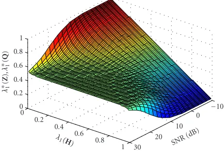
In Figure 5, the worst-case noise covariance matrix eigen-value λ1(Z) is shown over the SNR and the channel matrix eigenvalue λ1(H). The noise, channel, and transmit covari-ance matrices are sum-normalized, that is,λ1(Z)+λ2(Z)=1,
1
Figure 5: MIMO 2×2. Normalized worst-case noise covariance
matrix eigenvalueλ1(Z) and normalized optimal transmit
covari-ance matrix eigenvalueλ1(Q) over SNR (dB) and channel matrix
eigenvalueλ1(H).
over SNR (dB) and channel matrix eigenvalueλ1(H).
In Figure 5, we observe that for small SNR values the worst-case noise eigenvalues correspond to the channel ma-trix eigenvalues as predicted by (22). For high SNR val-ues, the worst-case noise eigenvalues have equal power. In Figure 6, we show the mutual information which is achieved byλ1(Z) andλ1(Q) fromFigure 5.
7. CONCLUSION
In this work, the instantaneous capacity of a MIMO sys-tem with worst-case noise was studied. The three different noise scenarios lead to different noise constraints and dif-ferent worst-case noise capacities. We studied a trace con-straint, fixed noise eigenvalues but free noise directions, and fixed diagonal entries in noise covariance matrixZbut free color of noise. In all three scenarios, the MIMO system lost its ability to cooperate at the transmitter side. In the first case with worst-case noise and trace constraint, the CSI at the transmitter dropped away. In scenario II and scenario III,
the eigendirections of the transmit covariance matrices were canceled by the worst-case noise direction or color and only power allocation could be performed at the transmitter.
APPENDICES
The last equality in (A.2) follows from the fact that the opti-mal eigenvectors ofQare equal to identity. The LHS of (A.2) does not depend onΛZ. Next, we show usingTheorem 1that
CI≥CDI. WithTheorem 1, we have
The maximum overQof the term in (A.3) is greater than or equal to the term with the choice ofUQ=UHH, that is,
Inequality (A.4) is valid for allZ. Therefore, we have
From (A.5), it follows that
CI≥CDI. (A.6)
From (A.2) and (A.6) followsCI = CID. This completes the proof.
B. PROOF OF LEMMA2
The proof ofLemma 2can be described as follows. Choose the eigenvalues of the noise covariance matrix to be equal to the weighted eigenvalues of the transmit covariance ma-trix, that is,λi(Q) = ρλi(Z), and show that the optimality
conditions for the minimization with respect toZis fulfilled. Choose the eigenvalues of the transmit covariance matrix to be equal to the weighted eigenvalues of the noise covariance matrix and show that the optimality conditions for the max-imization with respect toQare fulfilled.
We denote the optimal transmit covariance matrix eigen-values byλ∗i(Q) and the worst-case noise covariance matrix eigenvalues byλ∗i(Z). The waterfilling solution of the trans-mit covariance matrix eigenvalues is given for allλ∗i(Q)>0 as
λ∗
i (Q)=ξ−λ
∗
i(Z)
λi(H) (B.1)
withξ > 0. We show that the choice λ∗i(Z) = (1/ρ)λ∗i(Q) fulfills both optimality conditions (18) and (B.1), simulta-neously. This result is derived by computing the Lagrangian multiplier for (B.1) and (18) and showing thatξ=1/µ. From (18), we have forλ∗i (Q)=ρλ∗
i(Z),
λ∗
i(Z)=12ρλi∗(Z)λi(H) ·
1 + 4
ρλi(H)λ∗i(Z)µ−1
.
(B.2)
Solving (B.2) forµyields
1
µ=λ∗i(Z)
1
ρλi(H)+ 1
. (B.3)
From (B.1), we have forλ∗i(Z)=(1/ρ)λ∗i (Q),
λ∗
i(Q)=ξ− λ
∗
i(Q)
ρλi(H). (B.4)
Solving (B.4) forξgives
ξ=λ∗
i(Q)
1
ρλi(H)+ 1
= 1µ. (B.5)
Equation (B.5) connects the Lagrangian multiplier for the transmit covariance matrix optimization in (B.1) and the worst-case noise optimization in (18). This shows that
λ∗
i(Q)=ρλ∗i(Z) solves (B.1) and (18).
The closed-form expression forλ∗i(Q) in (19) is easily obtained from the power constraint:
m
k=1
λ∗
i (Q)=P. (B.6)
ACKNOWLEDGMENTS
Parts of this work was presented at the IEEE International Symposium on Signal Processing and Information Technol-ogy, Darmstadt, December 2003. This work was supported in part by the Bundesministerium f¨ur Bildung und Forschung (BMBF) under Grant BU150.
REFERENCES
[1] E. Telatar, “Capacity of multi-antenna Gaussian channels,”
European Transactions on Telecommunications, vol. 10, no. 6, pp. 585–595, 1999.
[2] G. J. Foschini and M. J. Gans, “On limits of wireless commu-nications in a fading environment when using multiple an-tennas,” Wireless Personal Communications, vol. 6, no. 3, pp. 311–335, 1998.
[3] H. Boche and E. A. Jorswieck, “Sum capacity optimization of the MIMO Gaussian MAC,” in Proc. 5th International Symposium on Wireless Personal Multimedia Communications (WPMC ’02), vol. 1, pp. 130–134, Sheraton Waikiki, Hon-olulu, Hawaii, USA, October 2002.
[4] H. Boche, M. Schubert, and E. A. Jorswieck, “Throughput maximization for the multiuser MIMO broadcast channel,” inProc. IEEE Int. Conf. Acoustics, Speech, Signal Processing (ICASSP ’03), vol. 4, pp. 808–811, Hong Kong, China, April 2003.
[5] H. Boche, M. Schubert, and E. A. Jorswieck, “Trace balancing for multiuser MIMO downlink transmission,” inProc. 36th Asilomar Conference on Signals, Systems and Computers (Asilo-mar ’02), vol. 2, pp. 1379–1383, Pacific Grove, Calif, USA, November 2002.
[6] M. Schubert and H. Boche, “Throughput maximization for uplink and downlink beamforming with independent cod-ing,” inProc. 37th Conference on Information Sciences and Sys-tems (CISS ’03), Baltimore, Md, USA, March 2003.
[7] E. A. Jorswieck and H. Boche, “Transmission strategies for the MIMO MAC with MMSE receiver: average MSE optimization and achievable individual MSE region,” IEEE Trans. Signal Processing, vol. 51, no. 11, pp. 2872–2881, 2003.
[8] S. N. Diggavi and T. M. Cover, “The worst additive noise un-der a covariance constraint,”IEEE Transactions on Information Theory, vol. 47, no. 7, pp. 3072–3081, 2001.
[9] S. Vishwanath, S. Boyd, and A. Goldsmith, “Worst-case ca-pacity of Gaussian vector channels,” inProc. 8th IEEE Cana-dian Workshop on Information Theory (CWIT ’03), Waterloo, Ontario, Canada, May 2003.
[10] H. Sato, “An outer bound to the capacity region of broadcast channels,” IEEE Transactions on Information Theory, vol. 24, no. 3, pp. 374–377, 1978.
[11] S. Vishwanath, N. Jindal, and A. Goldsmith, “Duality, achiev-able rates, and sum-rate capacity of Gaussian MIMO broad-cast channels,” IEEE Transactions on Information Theory, vol. 49, no. 10, pp. 2658–2668, 2003.
[13] R. S. Blum, “MIMO capacity with interference,”IEEE Journal on Selected Areas in Communications, vol. 21, no. 5, pp. 793– 801, 2003.
[14] S. Ye and R. S. Blum, “Optimized signaling for MIMO inter-ference systems with feedback,”IEEE Trans. Signal Processing, vol. 51, no. 11, pp. 2839–2848, 2003.
[15] W. Yu, W. Rhee, S. Boyd, and J. M. Cioffi, “Iterative water-filling for Gaussian vector multiple-access channels,” IEEE Transactions on Information Theory, vol. 50, no. 1, pp. 145– 152, 2004.
[16] P. Wolniansky, G. Foschini, G. Golden, and R. Valenzuela, “V-BLAST: an architecture for realizing very high data rates over the rich-scattering wireless channel,” inProc. URSI Interna-tional Symposium on Signals, Systems, and Electronics (ISSSE ’98), pp. 295–300, Pisa, Italy, September–October 1998. [17] D. P. Palomar, J. M. Cioffi, and M. A. Lagunas, “Uniform
power allocation in MIMO channels: a game-theoretic ap-proach,” IEEE Transactions on Information Theory, vol. 49, no. 7, pp. 1707–1727, 2003.
[18] M. Godavarti, A. O. Hero, and T. Marzetta, “Min-capacity of a multiple-antenna wireless channel in a static Rician fad-ing environment,” inProc. IEEE International Symposium on Information Theory (ISIT ’01), p. 57, Washington, DC, USA, June 2001.
[19] W. Yu, The Structure of the Worst-Noise in Gaussian Vector Broadcast Channels, Discrete Mathematics and Theoretical Computer Science (DIMACS) Series on Network Informa-tion Theory. American Mathematical Society, Providence, RI, USA, 2003.
[20] K. Fan, “Minimax theorems,” Proceedings of the National Academy of Sciences of the United States of America, vol. 39, pp. 42–47, 1953.
[21] T. M. Cover and J. A. Thomas, “Determinant inequalities via information theory,” SIAM Journal on Matrix Analysis and Applications, vol. 9, no. 3, pp. 384–392, 1988.
[22] M. Fiedler, “Bounds for the determinant of the sum of her-mitian matrices,” Proceedings of the American Mathematical Society, vol. 30, no. 1, pp. 27–31, 1971.
[23] A. W. Marshall and I. Olkin, Inequalities: Theory of Ma-jorization and Its Applications, vol. 143 ofMathematics in Sci-ence and Engineering, Academic Press, New York, NY, USA, 1979.
[24] P. Viswanath and D. N. C. Tse, “Sum capacity of the vec-tor Gaussian broadcast channel and uplink-downlink dual-ity,” IEEE Transactions on Information Theory, vol. 49, no. 8, pp. 1912–1921, 2003.
[25] S.-P. Wu, L. Vandenberghe, and S. Boyd, MAXDET: soft-ware for determinant maximization problems, May 1996,
http://www.stanford.edu/∼boyd/MAXDET.html.
E. A. Jorswieck studied at the Technis-che Universit¨at Berlin, Germany, where he graduated with Dipl.-Ing. in electrical en-gineering and computer science in 2000. He has been with the Fraunhofer Institute for Telecommunications, Heinrich-Hertz-Institut (HHI), Berlin, since 2001. He is also pursuing a Ph.D. degree in electrical engi-neering and computer science at the Tech-nische Universit¨at Berlin. His research
ac-tivities comprises performance and capacity analysis of wireless sys-tems and optimal transmission strategies for single-user and mul-tiuser MIMO systems.
H. Bochereceived his M.S. and Ph.D. de-grees in electrical engineering from the Technische Universit¨at Dresden, Germany, in 1990 and 1994, respectively. In 1992, he graduated in mathematics from the Tech-nische Universit¨at Dresden. From 1994 to 1997, he did postgraduate studies in mathe-matics at the Friedrich-Schiller Universit¨at Jena, Germany. In 1997, Dr. Boche joined Fraunhofer Institute for