Simulations of P SV wave scattering due to cracks by the 2 D finite difference method

Simulations of

P-SV

wave scattering due to cracks by

the 2-D finite difference method

Yuji Suzuki1∗_{, Takahiro Shiina}2†_{, Jun Kawahara}3_{, Taro Okamoto}4_{, and Kaoru Miyashita}3

1_{Graduate School of Science and Engineering, Ibaraki University, Mito 310-8512, Japan} 2_{Research Center for Prediction of Earthquakes and Volcanic Eruptions, Graduate School of Science,}

Tohoku University, Sendai 980-8578, Japan

3_{Faculty of Science, Ibaraki University, Mito 310-8512, Japan}

4_{Department of Earth and Planetary Sciences, Tokyo Institute of Technology, Tokyo 152-8551, Japan} (Received September 3, 2012; Revised June 20, 2013; Accepted June 25, 2013; Online published December 6, 2013)

We simulateP-SV wave scattering by 2-D parallel cracks using the finite difference method (FDM). Here, special emphasis is put on simplicity; we apply a standard FDM (second-order velocity-stress scheme with a staggered grid) to media including traction-free, infinitesimally thin cracks, which are expressed in a simple manner. As an accuracy test of the present method, we calculate the displacement discontinuity along an isolated crack caused by harmonic waves using the method, which is compared with the corresponding results based on a reliable boundary integral equation method. The test resultantly indicates that the present method yields sufficient accuracy. As an application of this method, we also simulate wave propagation in media with randomly distributed cracks. We experimentally determine the attenuation and velocity dispersion induced by scattering from the synthetic seismograms, using a waveform averaging technique. It is shown that the results are well explained by a theory based on the Foldy approximation, if the crack density is sufficiently low. The theory appears valid with a crack density up to at least 0.1 forSVwave incidence, whereas the validity limit appears lower forP wave incidence.

Key words:Scattering, cracked media, finite difference methods, attenuation, dispersion.

1.

Introduction

Random inhomogeneities inside the Earth’s lithosphere scatter high-frequency seismic waves and thereby cause phenomena such as the attenuation, dispersion, and genera-tion of coda waves (Satoet al., 2012). The modeling of such inhomogeneities can be categorized into two concepts: dom spatial fluctuation of medium parameters (called ran-dom media), and discrete scatterers such as cracks, inclu-sions, or cavities. Although the concept of random media has been popularly adopted in theoretically modeling seis-mic scattering (Satoet al., 2012), it assumes quite often a continuous heterogeneity. In contrast, the real Earth’s in-terior obviously has a discontinuous nature. It includes a large amount of cracks or fractures, and it also has many irregular interfaces having a sharp material contrast. Such a discontinuous heterogeneity can be modeled using the con-cept of discrete scatterers, either directly or approximately (Beniteset al., 1992).

One of the popular numerical methods to simulate seis-mic scattering due to discrete scatterers is the boundary

in-∗_{Now at: Systemlab Corporation, Tokyo 171-0022, Japan.}

†_{Formerly at: Faculty of Science, Ibaraki University, Mito 310-8512,} Japan.

Copyright cThe Society of Geomagnetism and Earth, Planetary and Space Sci-ences (SGEPSS); The Seismological Society of Japan; The Volcanological Society of Japan; The Geodetic Society of Japan; The Japanese Society for Planetary Sci-ences; TERRAPUB.

doi:10.5047/eps.2013.06.008

tegral equation method (BIEM) (e.g., Beniteset al., 1992; Murai et al., 1995; Pointer et al., 1998; Kelner et al., 1999; Liu and Zhang, 2001; Yomogida and Benites, 2002). The BIEM has often been believed to have advantages over domain-type methods in computational accuracy when dealing with discrete inhomogeneities (e.g., Beniteset al., 1992; Liu and Zhang, 2001), and in a great flexibility re-garding the shapes of scatterers. However, it also has short-comings: the difficulty in its application to the discrete scatterers embedded in matrices which themselves have a complex heterogeneity, computational costs that rapidly crease with the increasing numbers of scatterers, and the in-tractability for beginners to code their computer programs. Domain-type methods, such as the finite difference method (FDM) and the finite element method (FEM), are superior in these points.

A great advantage of the FDM is its high simplicity and tractability in general. Especially, the staggered-grid scheme (Virieux, 1984, 1986) has been known for its accuracy for media having large values of Poisson’s ra-tio (Moczo et al., 2002). In fact, with a proper assign-ment of medium parameters (Ohminato and Chouet, 1997; Okamoto and Takenaka, 2005; Takenaka et al., 2009), it is now possible to simulate wave propagation in media with large material contrasts such as irregular land topog-raphy (i.e., irregular free surface), irregular ocean-bottom topography (i.e., irregular liquid-solid interface), and three-dimensional heterogeneity including low-velocity soft sed-iments by using the staggered-grid scheme (e.g., Nakamura

et al., 2012; Okamotoet al., 2012, 2013).

However, the incorporation of cracks into the grids is not so straightforward. Some authors modeled cracks in indirect manners, such as thin layers of equivalent homoge-neous anisotropic materials (Vlastoset al., 2003) or arrayed point sources (van Antwerpen et al., 2002). In contrast, Saenger et al. (2000) modeled cracks as a thin inclusion with zero elastic constants and small mass density within the “rotated staggered grid” developed by them. An advan-tage of this method is the ability to treat cracks with arbi-trary shapes and orientations and even with intersections. Using this method, Saenger and his coworkers have numer-ically investigated the effective elastic moduli of cracked media (Saenger and Shapiro, 2002; Orlowskyet al., 2003; Saengeret al., 2004, 2006). Kr¨ugeret al.(2005) also ap-plied the method to the scattering and diffraction of anSH wave by a 2-D crack and demonstrated its high accuracy in comparison with an analytical solution.

The FEM has also been used for evaluating the ef-fective elastic moduli of cracked media, though mostly adopted in simulations of elastostatic deformation rather than wave propagation (Dahm and Becker, 1998; Grechka and Kachanov, 2006; Grechka, 2007). Frehner and Schmal-holz (2010) successfully applied the FEM to simulations of Stoneley guided waves around a fluid-filled fracture. Frehneret al.(2008) compared the FEM and the FDM ap-plied to the same problem ofP-SVwave scattering due to a 2-D circular inclusion. They concluded that the FEM is superior to the FDM in terms of computational time be-cause the former provides the same numerical accuracy with much less numerical grid points for modeling the curved interface of an inhomogeneity. A disadvantage of the FEM is that it is somewhat more complex to implement than the FDM and often needs a third-party software for mesh generation.

In our previous paper (Suzukiet al., 2006; hereafter re-ferred to as Paper I), we numerically simulatedSH wave scattering due to traction-free, infinitesimally thin cracks by the 2-D FDM. Therein was proposed a new, simple and cost-effective simulation technique; we adopted a standard velocity-stress FDM (Virieux, 1984; Levander, 1988) and expressed cracks in a staggered grid just by arraying grid points with zero shear traction. This is a natural extension of the FDM-based simulations of crack propagation originated by Madariaga (1976), in which the boundary conditions on the crack planes can be directly given. It was much simpler than the FDM previously proposed to deal with cracked me-dia, though its application was limited to cracks parallel to the grid lines. We proved that this technique successfully deals with SH wave scattering due to cracks with practi-cally sufficient accuracy, through accuracy tests based on the comparison with reliable BIEM estimates (Muraiet al., 1995). It remained, however, to be extended to 2-DP-SV or 3-D elastic wave scattering, which would be practically more important.

An interesting topic on cracked media is the attenuation and velocity dispersion of waves propagating therein. Theo-retically, they can be predicted by a stochastic theory based on Foldy’s (1945) approximation. This approximation is based on the assumption of many scatterers distributed

ran-domly and sparsely (Ishimaru, 1978), and it is expected to give results accurate to the first order in the distribu-tion density (Keller, 1964). Although considerable efforts have been made to propose alternative approximations that are claimed to be valid for more densely distributed scat-terers, the original Foldy approximation theory (hereafter, FAT) has maintained its popularity probably because of its mathematical simplicity (Kawahara, 2011) and the lack of consensus on which approximation is best as an alterna-tive to the FAT (Kawaharaet al., 2009). The FAT was ap-plied to cracked media first by Kikuchi (1981a, b) and then by many authors in seismology and acoustics (Yamashita, 1990; Kawahara and Yamashita, 1992; Kawahara, 1992; Zhang and Gross, 1997; Caleap and Arist´egui, 2010). How-ever, its actual validity limit with respect to crack density remains unclear. Using their BIEM, Murai et al. (1995) simulatedSHwave scattering by randomly distributed 2-D cracks and determined the scattering attenuation and dis-persion experimentally, thus validating the FAT of Kawa-hara and Yamashita (1992) as long as the crack density is relatively low (≤ 0.02). Later, Murai (2007) revisited this problem and concluded that the FAT seems to be valid for a crack density up to at least 0.1. Unfortunately, the ordinary peak picking technique, as they used in their measurement, will not work for dense crack distributions, because the ini-tial motions of propagating waves will often be distorted too much to pick the peaks properly. In Paper I, we also performed numerical experiments like Muraiet al.(1995) and Murai (2007), though we adopted a waveform averag-ing method in measuraverag-ing the attenuation and dispersion. We showed that these parameters are obtained stably even for rather dense crack distributions, and revealed that the FAT works well for a crack density up to about 0.1, but probably not beyond it. To the authors’ knowledge, however, it has not been confirmed whether the same conclusion holds for P-SVwave scattering due to 2-D cracks.

The present article is a continuation of Paper I, and its purpose is two-fold. First, we extend the FDM of Paper I in order to simulateP-SVwave scattering due to 2-D traction-free, infinitesimally thin cracks (Section 2). We validate the method through an accuracy test, in which it is compared with a reliable BIEM in the calculation of the displacement discontinuity along a single crack (Section 3). Second, we examine the validity of the FAT concerningP-SVwave scat-tering due to many cracks on the basis of numerical exper-iments with the present simulation technique (Section 4). Discussion and conclusions are given in Section 5. As in Paper I, we treat only cracks parallel to the grid lines; the extension of the present method to the case of arbitrarily oriented cracks is discussed in Section 5.

2.

Finite Difference Method

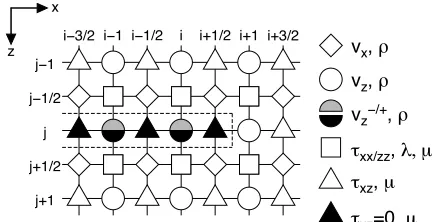
We adopt a 2-D velocity-stress finite difference scheme forP-SVwaves with the accuracy of second order in space as well as in time (Virieux, 1986). The algorithm is so stan-dard that it is described below only briefly. The staggered grid used in the present study is shown in Fig. 1. Here, the x- and z-axes are taken in the horizontal and vertical directions, respectively. We definevx andvz as the

Fig. 1. Staggered grid and implementation of cracks. Different symbols denote grid points on which different quantities are allocated as follows; diamonds: horizontal particle velocity and mass density; circles and semicircles: vertical particle velocity and mass density; squares: normal stress,λ, andμ; triangles: shear stress andμ. Here,λandμare the Lam´e parameters. The region enclosed by the dotted line corresponds to a crack, in which the solid triangles denote the points with zero shear stress. Each pair of gray and black semicircles denotes two close points located on the upper and lower crack faces, respectively, whose separation is much smaller than the grid spacing.

τzzas normal stress,τx zas inplane shear stress,λandμas

the Lam´e parameters, andρas mass density. The grid spac-ings in thex- andz-directions are assumed to have the same lengthh. Letting the time step bet, the finite difference scheme for this grid is expressed as:

vx(i−1₂,j−1₂,m+1₂)=vx(i−1₂,j−1₂,m−1₂)

We assume for the moment that cracks are horizontal (parallel to thex-axis). We impose the traction-free bound-ary conditionτx z=τzz=0 on the crack planes. The cracks

are incorporated into the grid in the following manner. First, we imposeτx z = 0 on a sequence of horizontally arrayed

grid points (solid triangles in Fig. 1) which define a crack plane. The crack tips are defined as the leftmost and right-most points of the array (e.g., the grid point(i + 1₂,j)in the figure). However, we cannot explicitly imposeτzz =0

on the crack plane thus defined, because the crack is com-posed of grid points forτx zand forvzbut not forτzz. Such

a difficulty was not encountered in Paper I, in which it was enough to let antiplane shear stress τx y only be zero.

Alternatively, we split here each grid point forvz on the

crack into two very close points, which respectively repre-sent the points on the upper and lower crack faces (the gray and black semicircles in Fig. 1). Since there arises a dis-placement discontinuity (Section 3), incorporation of such a split variable, or a “two-valued” variable, is inevitable in order to correctly express the response of an infinitesi-mally thin crack when the grid points for particle velocity (or displacement) are located on the crack plane. We ex-press the coordinates of these points as, say,(i,j ±δ), in whichδ may be regarded as half of the infinitesimal crack width with 0 < δ h. Introducing further the nota-tion asvz(i,j±δ,m−1₂)=vz±(i,j,m−12), we calculate v±

z (i,j,m+12)by the following scheme with either a

for-ward or backfor-ward difference with regard toτzzas:

v±

This scheme satisfies the boundary conditions on the crack planes as described in Appendix A. Note that Eq. (1b) requires the continuity of the displacement and, hence, it is only applicable to media without cracks. A similar equation to Eq. (2) was previously derived by Hayashidaet al.(1999) to express a free surface in a staggered grid for 3-D elastic media.

Then, in the vicinity of the crack, the normal stress

τx x(i,j±1₂,m+1)andτzz(i,j±1₂,m+1)are calculated

usingvz±(i,j,m+1₂)instead ofvz(i,j,m+1₂)in Eqs. (1c)

and (1d). Note that vertical cracks (parallel to thez-axis) can be also treated in almost the same manner. Although the above-mentioned manner to incorporate cracks into a grid may not be so simple as that for the case ofSH wave scat-tering given in Paper I, it still seems to retain simplicity as compared with those of other previous studies (Section 1).

In any simulation performed below, a plane wavelet is assumed to propagate upward (in the negativez-direction) from below and be incident on cracks either normally or parallel. Then, velocity seismograms are synthesized at specified grid points, which are finally integrated with the trapezoidal rule to yield the displacement seismograms. As in Paper I,h andt are chosen to satisfy the stability conditiont < h/√2αand the sampling criterionh<

β/n ful (Virieux, 1986; Moczo, 1998), in whichn=10 for

fulis the frequency up to which one needs to have accurate

results without the grid dispersion. For convenience, β,

ρ, and the crack half lengtha are set to be unity and the values of other parameters are normalized with them. We also assume a Poisson solid withλ = μand, hence,α =

√

3β. Concerning the artificial boundaries of the whole grid (model space), we impose again simple conditions. The cyclic boundary condition is applied to the left and right ends to express approximately an infinitely long cracked layer. A standard absorbing boundary condition of Clayton and Engquist (1977) is assumed along the top and bottom ends. Although artificial reflections from the absorbing boundaries cannot be perfectly erased, we actually analyze the portions of seismograms not contaminated with them.

3.

Crack Displacement Discontinuity

As in Paper I, we compare the results of our FDM sim-ulations with those based on a frequency-domain BIEM, thus trying to validate the present simulation method. For this purpose, we calculate the displacement discontinuity along a single crack caused by incident harmonic waves, using both methods. Note that the normal displacement dis-continuity (NDD) along a traction-free, infinitesimally thin crack due to normally incident harmonicPwaves was ana-lytically solved by Mal (1970). Kawahara and Yamashita (1992) developed a BIEM algorithm for treating an iso-lated crack, which reproduces Mal’s results quite excel-lently. Hence, we infer their BIEM to be reliable and adopt it here. In order to treat the BIEM results as the correct answers, we make the discretization interval of the crack planes in the BIEM calculation to be much smaller than the crack length as well as the wavelength, as in Paper I.

The manner of the FDM calculation of the crack dis-placement discontinuity is the same as that in Paper I. Con-sider an isolated horizontal crack with the length 2a. Let a quasi-monochromatic wave train

u0(x,z,t)=b H(lz+ωt)sin(lz+ωt) (3)

propagate upward and then impinge normally on the crack, in whichbis the amplitude,ωis the angular frequency and H( )is the Heaviside step function. The wave mode is ei-therPorSV;landu0_{, respectively, denote theP}

wavenum-berh =ω/αand the vertical displacement for the former, whereas they denote theS wavenumberk = ω/βand the horizontal displacement for the latter. Note thath =k/√3 becauseα = √3β. The wave incidence causes the oscil-lation of the crack faces, which approaches the stationary state with the increasing lapse time. We evaluate the am-plitudes of the oscillatory displacement discontinuity along the crack when the oscillation appears almost stationary. Since the shear displacement discontinuity (SDD) cannot be defined directly at the grid points on the crack plane, we instead measure the differences of thex-component dis-placement seismograms calculated at the pairs of points just above and below the plane (e.g., the points(i−1

2,j± 1 2)in

Fig. 1), and then take their amplitudes. The approximation errors due to the offsets of the measurement points from the crack plane would be small ifh is sufficiently small. In contrast, the NDD can be defined directly on the crack plane (e.g., the grid point(i,j)in Fig. 1); that is, it is calculated

Fig. 2. Oscillation of both faces of an isolated crack due to the incidence of a quasi-monochromaticPwave train (ka=2.4,ha=1.39) observed at around the center of the crack. The panels with ‘Hor.’ and ‘Vert.’ indicate horizontal and vertical displacement, respectively. (a) Seismo-grams for a horizontal crack due to normal wave incidence. Solid and dashed curves correspond to the upper (shaded) and lower (illuminated) faces, respectively. In the upper panel, the solid curve masks the dashed one. (b) Seismograms for a vertical crack due to parallel wave inci-dence. Solid and dashed curves correspond to the left and right crack faces, respectively. In the lower panel, the solid curve masks the dashed one.

from the time integration of v+z −v−z at the same points.

We also examine the case of an isolated vertical crack, on which waves impinge parallel to the crack. The NDD and SDD along the crack are then defined in a similar manner.

We set heret =0.003a/βandh =0.0125a. Choos-ing the same values of the parameters, the second-order FDM adopted in Paper I gave an SDD which was highly consistent with those by the BIEM, independently of the wavenumbers. Note that the fourth-order FDM was shown to systematically underestimate the SDD (by several per-cent), probably because of the nonlocality of the finite dif-ference operator; see Paper I as to the detailed discussion. We use here the second-order FDM throughout. Note also that the present choice ofh and the sampling criterion (Section 2) require an inequality ful <8.0β/awhereas the

incident waves considered here (and also in Section 4) are shown to have a negligibly small energy for a frequency be-yond 8.0β/a(corresponding toka>50). This implies that every simulation will not suffer grid dispersion.

Fig. 3. Displacement discontinuity along an isolated crack due to a normal incidence of harmonicPorSVwaves: (a) normal displacement discontinuity due toPwaves, and (b) shear displacement discontinuity due toSVwaves. The abscissas represent the distance from the center of the crack. The curve parameters denoteka. The solid and dashed lines indicate the calculations based on the present FDM and the BIEM of Kawahara and Yamashita (1992), respectively.

of the incident wave. The NDD or SDD will be obtained from the difference of the pair of seismograms in each panel. We notice that the normal incidence of the P wave on the horizontal crack causes only a vertical displacement on the crack faces (Fig. 2(a)). In contrast, the parallel inci-dence of the Pwave on the vertical crack makes the crack faces oscillate vertically as well as horizontally, though the vertical displacement of both crack faces are always equal (Fig. 2(b)). These features are recognized irrespective of the positions along the crack and the wavenumbers of the incident waves, implying that the SDD never occurs for P waves incident either normal or parallel to a crack, as ex-pected. Similarly, we also confirmed that the NDD never occurs for either a normal or parallel incidence ofSVwaves (figure omitted).

In the following, we show only the results on non-zero NDD and SDD. Their values are normalized withhandk forPandSwave incidence, respectively, after Mal (1970). Note that the same normalization was also employed in figure 2 of Paper I, but without mention.

Figure 3(a) denotes the NDD due to the normalP wave incidence for the normalized S wavenumberka = 0, 0.8, 2.4, 3.6, and 5.2 (normalizedPwavemunberha=0, 0.46, 1.39, 2.08, and 3.00, respectively) after Mal (1970); the cor-responding P wavelengths are ∞, 13.6a, 4.5a, 3.0a, and 2.1a, respectively. Since the displacement discontinuity for ka = 0 cannot be calculated by the present time-domain FDM, we show only the BIEM estimates in this static case. Note that the discontinuity is always symmetrical with re-spect to the center of the crack for normal wave incidence. The figure shows good agreement between the FDM and BIEM estimates for every positiveka.

Figure 3(b) denotes the SDD due to the normalSVwave incidence for the normalized S wavenumberka = 0, 1.0, 2.8, 4.2, and 6.0; the corresponding Swavelengths are∞, 6.3a, 2.2a, 1.5a, and 1.0a, respectively. Note that the same values ofka were chosen in Paper I for the accuracy test

of its FDM calculations after Mal (1970). In this case, the discontinuity by the FDM does not vanish outside the crack (at a distance larger than 1.0ain the figure). As mentioned in Paper I, this can be explained by the offsets of the mea-surement points from the crack plane, and, therefore, gets smaller for smallerh. Thus, it does not imply the fail-ure of the present FDM. Except for this, the agreement be-tween the FDM and BIEM estimates is satisfactory also in this case. Note that the agreement seems slightly worse than that seen in Fig. 3(a), especially forka=1. This may also be explained by the offsets of the measurement points stated above.

The results on NDD and SDD for parallelPandSVwave incidence are shown in Figs. 4(a) and 4(b), respectively. In these cases, the discontinuity is not symmetrical with respect to the center of the crack except for the static limit (ka = 0), so that it needs to be displayed over the whole crack. The overall features of the figures are the same as those seen in Figs. 3(a) and 3(b); the FDM and BIEM estimates are again consistent for both P and SV wave incidence and for every positive wavenumber.

In summary, the present FDM produces the crack dis-placement discontinuity due to either P orSV wave inci-dence fairly accurately, independently of wavenumbers. We therefore conclude that the present method is applicable to the synthesis ofP-SVwaves scattered by cracks.

4.

Validation of the Foldy Approximation Theory

ap-Fig. 4. Displacement discontinuity along an isolated crack due to a parallel incidence of harmonicPorSVwaves: (a) normal displacement discontinuity due toPwaves, and (b) shear displacement discontinuity due toSVwaves. The abscissas represent the positions relative to the center of the crack. The rightward arrows indicate the direction of wave propagation relative to the crack plane. The curve parameters denoteka. The solid and dashed lines indicate the calculations based on the present FDM and the BIEM of Kawahara and Yamashita (1992), respectively.

Table 1. Parameters of the crack distribution models used in the simulations.PandSVindicate the wave modes.HandVindicate the horizontal and vertical cracks (normal and parallel wave incidence), respectively.

Model Wave/Cracks N W×L ND

1 P/H,P/V,SV/H,SV/V 19 40a×38a 0.0125 6

2a P/H,SV/H,SV/V 36 40a×18a 0.05 12

2b P/V 76 40a×38a 0.05 12

3a P/H,SV/H,SV/V 32 40a× 8a 0.1 18

3b P/V 152 40a×38a 0.1 18

proximation in which the waves effectively impinging on each scatterer (crack) are equal to the waves that would be observed without the scatterer. This approximation, first in-troduced by Foldy (1945), yields a closed equation for mean waves, called the Foldy-Twersky integral equation (Ishi-maru, 1978). Kawahara and Yamashita (1992) solved it for P-SVas well asSHwave scattering due to cracks filled with an incompressible viscous fluid, and obtained the attenua-tion and phase velocity of the mean waves to the first order in the crack density. Kawahara (1992) then analyzed the case forP-SVwave scattering due to empty (traction-free) cracks. In Paper I, we validated in a numerical-experimental manner the FAT of Kawahara and Yamashita onSH wave scattering in the case of cracks filled with an inviscid fluid (or equivalently, shear stress-free cracks); the same experi-mental procedures are again adopted here, which are sum-marized below.

4.1 Outline of the simulations

First, we assumeN cracks with a length of 2a inside a rectangular area with a horizontal size of W and vertical size ofL. The cracks are distributed in such a manner as visualized in figure 8 of Paper I; that is, they are located almost randomly, except for the non-overlapping constraint that the interval between any two points belonging respec-tively to any two crack planes must be greater than 0.15a. Here, the 2-D crack density is defined as = N a2_{/W L.}

Second, we array 100 receivers evenly along a horizontal

line 2aabove the top end of the crack distribution area. We then let a plane wavelet be vertically incident on the bot-tom end from below, and synthesize seismograms at the re-ceivers using the FDM. We adopt here an incident wavelet whose source time function is given as the first derivative of a Gaussian function; see equations (4), (5) and figure 7 of Paper I as to the details. The peak frequency of its power spectrum is 1/√π ≈0.56 in the unit ofβ/a, correspond-ing toka =2√π ≈3.5 andha =2√π/3 ≈2.0. Third, we average the seismograms for all the receivers to obtain a “spatial-averaged seismogram”. Here, we assume ergod-icity, i.e., we assume that ensemble averaging can be re-placed with spatial averaging (Shapiro and Kneib, 1993). Fourth, we repeat the simulation and averaging process as stated above for NDdifferent realizations of the crack

dis-tribution that are stochastically identical but are generated using different random number series. Thus, ND

vfrom the spectral ratio of the synthetic mean wave to the initial wavelet that would be observed without the cracks, C(ω); after some calculation, we obtain:

C(ω)=exp

in which “Im” and “Re” denote the imaginary and real parts, respectively. The obtainedQ−1 _{andv are to be compared}

with the values predicted by the FAT under the assumption that the mean wave is of the same mode (either P orSV) as that of the initial wavelet. Practically, we evaluate these quantities only for some frequency band inside which the initial wavelet has a sufficiently high energy for the sake of an accurate calculation. Instead of evaluating the estimation errors of Q−1 and v directly, we calculate the standard deviation of the synthetic mean wave and regard it as the error range. We also compute the waveform predicted by the FAT (“predicted mean wave”). If the predicted mean wave coincides with the synthetic mean wave within the error range, we regard their coincidence as significant.

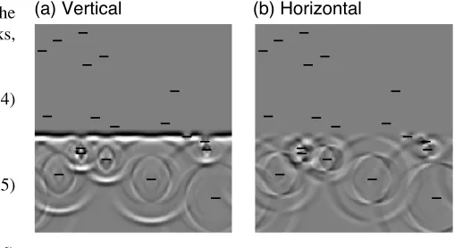
In every simulation performed, we sett = 0.003a/β andh =0.0125a as in the preceding section. Other pa-rameters of the crack distribution models used are summa-rized in Table 1. An example of the snapshot of a simulated wavefield is shown in Fig. 5, in which scattered waves from individual cracks are clearly seen.

We notice that Shapiro and Kneib (1993) have stated that spatial averaging works well if the length of the receiver ar-ray is much larger than max(acl, λ_wl), in which acl is the

correlation length of the medium heterogeneity andλwlis a

wavelength; in such cases, the incoherent part of a wavefield would interfere destructively during the spatial averaging process and only the coherent part (mean wave) would be retained. In the present simulation geometry,aclnearly

cor-responds to the size of the scatterers (cracks) 2a(Kawahara, 2011), which is much smaller than the length of the receiver arrayW =40a(Table 1). However, the wavelengths are not always sufficiently smaller thanW. As seen in the follow-ing subsections, we will numerically evaluate Q−1 _andv

for 0.5<ka<10 (0.29<ha<5.77) in which the initial wavelet has a high energy. This wavenumber range corre-sponds to 21.8a > λP >1.1aand 12.6a > λS >0.6a, in

whichλP andλS are P and S wavelengths, respectively.

Hence, W is only a few times larger than the maximum wavelength of either the P or theS wave corresponding to ka=0.5. As a result, the spatial averaging of seismograms for only one realization of a crack distribution removes the incoherent waves only partially, and, hence, the ensemble averaging process among many realizations is required for the total removal of the incoherent waves. Actually, we chose NDin Table 1 to achieve this purpose by increasing

NDuntil coda-like wave trains effectively vanish from the

synthetic mean wave.

Fig. 5. Snapshot of aP wave propagating upward through a cracked region (a realization of Model 1). Black and white indicate positive and negative values of displacement, respectively. Short horizontal black lines indicate cracks. (a) Vertical and (b) horizontal displacement.

4.2 Results for sparsely distributed cracks

We first demonstrate the results for Model 1, with which the crack density is so low ( = 0.0125) that the FAT is expected to be sufficiently valid. The result for the case of P wave incidence on horizontal cracks is shown in Fig. 6. In Figs. 6(a) and (b), we plot ND×100 horizontal- and

vertical-component seismograms, respectively. Here, we also show the traces of the synthetic mean wave and its stan-dard deviation (error range) derived from the seismograms; the initial wavelet without the cracks is also plotted for ref-erence. In Fig. 6(a) (see also Fig. 6(c) as the close-up), one may clearly observe the attenuation on the primary part of the synthetic mean wave (25<t <27 in unit ofa/β). The primary wave is also followed by a pulse of relatively long duration (around 27<t <32). However, the trace does not contain a coda-like long wave train, implying that the aver-aging process has successfully removed coda waves. We further plot the trace of the predicted mean wave in the fig-ure. The agreement between the synthetic and predicted mean waves is considerably good. This also suggests that the above-mentioned pulse after the primary wave would be attributed to the waveform dispersion of the initial wavelet due to scattering. Note that such a feature of the wave traces was previously reported in Paper I forSH wave incidence (figure 9 thereof). In contrast, Fig. 6(b) indicates that the horizontal component of the synthetic mean wave contin-ues to be effectively zero despite the high amplitude of each synthetic seismogram. This validates the assumption of the FAT that the modes of the mean wave and the initial wavelet are the same (Subsection 4.1), though P-to-S conversion scattering significantly occurs.

The values ofQ−1_{andvderived from the synthetic and}

Fig. 6. (Color online) Results of the simulations obtained for Model 1 (=0.0125) withPwave incidence on horizontal cracks. (a) Vertical- and (b) horizontal-component synthetic seismograms (the cloud of thin light blue lines), and the synthetic mean wave and its standard deviation derived from these seismograms (solid and dotted blue curves, respectively). The predicted mean wave is indicated by the red curve, though almost masked by the solid blue one. The thin black curve denotes the initial wavelet that would be observed without the cracks. (c) The close-up of the primary part in (a). The synthetic seismograms are omitted. (d)Q−1_{, and (e)vfor the synthetic mean wave (blue curves). The prediction by the FAT is denoted by red} curves.

in Fig. 6(a).

The result for the same model but for the case ofSVwave incidence on horizontal cracks is depicted in Fig. 7. A no-ticeable feature of Fig. 7(a) is that incoherent wave motion exists at each synthetic seismogram prior to the arrival of the primarySV wave. This motion will be attributed toS -to-P conversion scattering due to cracks; after averaging, it effectively vanishes from the trace of the synthetic mean wave, just as the later coda waves. Except for this differ-ence, the overall features of Fig. 7 are quite similar to those of Fig. 6: the mean wave is of the same mode as that of the initial wavelet, and its waveform, attenuation, and disper-sion are described by the FAT satisfactorily.

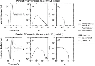
Figure 8 shows the results for the same model but for the case of P- andSV-waves incident on vertical cracks, supporting again the validity of the FAT for such sparse dis-tributions of cracks. It might be interesting that the disper-sive deformation of the mean waveforms is rather signifi-cant forSV wave incidence on vertical cracks (Fig. 8(d)). In this case, a new peak, which is not recognized for the ini-tial wavelet, emerges prior to the primary trough (at around t =44.2). This may be related to the somewhat abnormal

shapes of the curves ofQ−1_{andvindicated in Figs. 8(e)}

and 8(f).

4.3 Results for more densely distributed cracks

We next show the results for the models with denser distributions (Models 2 and 3), focusing on the validity limit of the FAT.

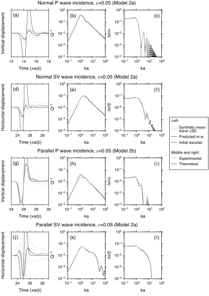
Figure 9 depicts the results for Model 2 (2a or 2b) with a crack density = 0.05. Note that the case of P wave incidence on vertical cracks was examined on the basis of Model 2b unlike the other three cases, which has more cracks and a wider space than Model 2a adopted for the latter cases (Table 1). It is because that the Q−1 andv are rather small in this case, as indicated by Figs. 9(h) and 9(i), so that a large travel distance seems to be preferable for measuring them. In Fig. 9, we may still recognize the fairly good agreement between the experimental and theoretical results on the whole. An exception is the case of P wave incidence on the vertical cracks, in which a notable discrep-ancy exists between the experimental and theoretical values of eitherQ−1_{orv(Figs. 9(h) and 9(i)). Nevertheless, the}

phe-Fig. 7. (Color online) Results of the simulations obtained for Model 1 ( =0.0125) with anSVwave incidence on horizontal cracks, shown in the same manner as in Fig. 6. (a) Horizontal- and (b) vertical-component synthetic seismograms, and the synthetic mean wave and its standard deviation derived from these seismograms. The synthetic mean wave and initial wavelet, if without the cracks, are also depicted. (b) The close-up of the primary part in (c), though without the synthetic seismograms. (d)Q−1_{, and (e)vfor the synthetic and predicted mean waves.}

nomenon may be explained by the fact that the discrepancy between the experimental and theoretical values of Q−1 _or vis mainly limited toka<2, whereas both the synthetic and predicted mean waves can be shown to have a high en-ergy for 1.5<ka<4. This implies that the waveforms of both mean waves are dominated by their respective spectral contents in the range 1.5<ka<4. Furthermore, these two spectral contents are similar because the experimental and theoretical values ofQ−1_{orvare close in this}

wavenum-ber range. In contrast, the primary peaks and troughs of the mean waves are somewhat overestimated by the FAT for horizontal cracks (Figs. 9(a) and 9(d)), which may cor-respond to the slight underestimation ofQ−1by the FAT at aroundka=3.5 (Figs. 9(b) and 9(e)).

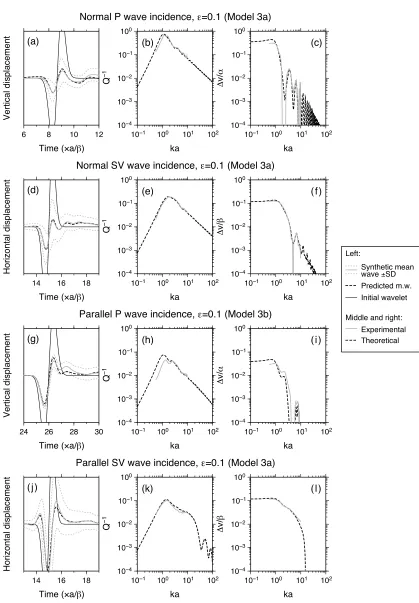
The results for Model 3 (3a or 3b) with a higher crack density ( =0.1) are depicted in Fig. 10. Now the overes-timation of Q−1 _{andvby the FAT forka < 2 is rather}

remarkable for P wave incidence on the vertical cracks (Figs. 10(h) and 10(i)). In this case, the trace of the pre-dicted mean wave almost deviates from the error range of the synthetic mean wave, though temporarily (at around t = 27.5) (Fig. 10(g)). The same tendency is also recog-nized, though more weakly, for P wave incidence on the horizontal cracks (Figs. 10(b) and 10(c)). Such a feature

was previously reported in Paper I onSHwave scattering in the case of an even higher crack density ( =0.2) (Fig. 12 thereof). As discussed therein, this may be partly attributed to the effect of multiple scattering among closely located scatterers. The FAT is based on the randomness and sparse-ness of scatterer distributions as stated in Section 1. Speak-ing precisely, however, a distribution of non-overlappSpeak-ing scatterers cannot be perfectly random for a finite distribu-tion density. In the present case, with such dense distri-butions, the randomness would be largely degraded, which results in large approximation errors. Note that a more rig-orous treatment of mean waves revealed that the terms of order2, neglected in the FAT of Kawahara (1992), can be described in terms of such nonrandomness (Keller, 1964). Only in the case of P wave incidence on the horizontal cracks, may one also perceive the first motion of the pre-dicted mean wave prior to the onset of the initial wavelet without cracks (at aroundt =7.3), which is not observed for the synthetic case (Fig. 10(a)). Such apparently acausal wave motion was again reported in Paper I in the case of

= 0.2, which we attributed to a too strong attenuation (Q−1 _{∼ 1). Throughout the present paper, as well as}

Fig. 8. Results of the simulations obtained for Model 1 (=0.0125) with either (a–c)Por (d–f)SVwave incidence on vertical cracks. Left column (a, d): Synthetic mean waves and their standard deviation derived from synthetic seismograms (solid and dotted gray curves, respectively) of either (a) vertical- or (d) horizontal-component. The dashed black curves denote the predicted mean waves, and the thin solid black ones denote the initial wavelets, if without the cracks. Middle (b, e) and right (c, f) columns:Q−1andvfor the synthetic mean waves (solid gray curves), respectively. The prediction by the FAT is denoted by dashed black curves.

Strictly, however, it is an approximation valid for weak at-tenuation, i.e., Q−1 _{1 (e.g., Aki and Richards, 2002).}

This is obviously not satisfied in the present case, in which the maximum value of Q−1 _{is rather close to 1, probably}

making both the theory and measurement not very reliable. In contrast, the disagreement between the experimental and theoretical results still remains not very serious forSV wave incidence, even in the case of = 0.1 (Figs. 10(d) to 10(f) and 10(j) to 10(l)). One may therefore say that the FAT will be nearly valid at least up to =0.1 concerning SVwaves. This is consistent with the conclusion of Paper I as well as that of Murai (2007) onSHwave scattering.

We notice that the case of P wave incidence on verti-cal cracks with = 0.1 was examined on the basis of Model 3b withN =152, many more cracks than assumed in Model 3a adopted for the other three cases, for the same reason as before (Model 2). In Paper I, however, we re-vealed that the numerical errors of the FDM seem to weakly increase with an increasing number of cracks. Hence, one might infer that the failure of the FAT, in that case, is partly because of the numerical errors. To examine this infer-ence, we recalculate Q−1 andv for this case by replac-ing Model 3b with Model 3a. The result (not shown) is effectively unchanged from that depicted in Figs. 10(h) and 10(i), indicating that the FDM calculations were sufficiently accurate and the failure of the FAT, in this case, is not due to the numerical errors caused by too many cracks.

One may also infer that strong multiple scattering among the cracks enhances the numerical errors. This effect would be significant for a high crack density and especially for

high wavenumbers, even if the sampling criterion (Sec-tion 2) is satisfied. However, we confirmed that chang-ing h by a factor of two does not effectively change the numerical results for Model 3a for all the considered wavenumbers (figure omitted). This again verifies the ac-curacy of the present FDM simulations, even up to=0.1 and the considered wavenumbers.

In summary, we have confirmed that the FAT is actually valid for low crack density (say,∼0.01) for all the cases considered. Its validity limit with regard to , however, seems to depend on the wave modes and, sometimes, the incident angles of waves to cracks. The FAT would be nearly valid withup to at least 0.1 for the case ofSVwave incidence. In contrast, the validity limit of the FAT seems to be lower forP wave incidence. It may be, say, 0.05 for normal incidence, whereas even a lower value ofmay be preferable for a grazing incidence.

5.

Discussion and Conclusions

com-Fig. 9. Results of the simulations obtained for Model 2 (=0.05) with either (a–c)Por (d–f)SVwave incidence on horizontal cracks, and those with either (g–i)Por (j–l)SVwave incidence on vertical cracks, shown in the same manner as in Fig. 8. Left column (a, d, g, j): Synthetic mean waves and their standard deviation derived from synthetic seismograms of either (a, g) vertical- or (d, j) horizontal-component. The predicted mean waves and the initial wavelets, if without the cracks, are also depicted. Middle (b, e, h, k) and right (c, f, i, l) columns:Q−1_{andvfor the synthetic mean} waves, respectively.

pared this with the corresponding results based on a reli-able BIEM of Kawahara and Yamashita (1992). The test resultantly indicated that the present method yielded a suf-ficient accuracy for any wavenumber. As an application of

Fig. 10. Results of the simulations obtained for Model 3 (=0.1) with either (a–c)Por (d–f)SVwave incidence on horizontal cracks, and those with either (g–i)Por (j–l)SVwave incidence on vertical cracks, shown in the same manner as in Fig. 9. Left column (a, d, g, j): Synthetic mean waves and their standard deviation derived from synthetic seismograms of either (a, g) vertical- or (d, j) horizontal-component. The predicted mean waves and the initial wavelets, if without the cracks, are also depicted. Middle (b, e, h, k) and right (c, f, i, l) columns: Q−1_{andvfor the synthetic mean} waves, respectively.

synthetic seismograms, using a waveform averaging tech-nique. It was shown that the results are well described by the FAT of Kawahara (1992), if the crack densityis suf-ficiently low, say, 0.01. The FAT apparently remains to be

To the authors’ knowledge, the present study is the first one to have successfully validated the FAT for cracked me-dia, even if there exists mode conversion between PandS waves. Although we only dealt with the simplest type of cracks (i.e., parallel equal-sized traction-free cracks), some previous studies based similarly on numerical experiments showed that the FAT works well also for others kinds of cracks concerningSH wave scattering. The examples are cracks filled with a viscous fluid (Muraiet al., 1995), ran-domly oriented cracks (Yoshida et al., 2003), and cracks of unequal lengths (Paper I). On the basis of the same ap-proach as the present study, Kawahara et al. (2009) also proved that the FAT is nearly valid for SH wave scatter-ing due to 2-D round cavities—possibly identified with high-aspect-ratio cracks—with a volume concentration up to 0.1. All these results suggests that the validity of the FAT would be universal as long as the scatterers are sparsely dis-tributed, irrespective of the geometry and physical proper-ties (boundary conditions) of the cracks, the wave modes, and, possibly, the spatial dimensions.

In contrast, the validity limit of the FAT for cracked me-dia seems to depend on the wave modes. Moreover, this is as well as the incident angle in the case of Pwave inci-dence. The details of the dependence of the validity limit on the incident angle, however, remain unrevealed since we considered here only two kinds of incident angles (0◦and 90◦); the case of oblique wave incidence should be investi-gated in future. It also remains to be clarified why the valid-ity limit of the FAT seems to be lower forPwave incidence than forSVwave incidence.

As stated in Section 4, the overestimation by the FAT of Q−1 _{andv observed for P waves in densely cracked}

media (Fig. 10) may be partly attributed to the imperfect randomness of distributions enhanced with an increasing. This implies that the validity of the FAT would be limited not only by but also by the spatial correlation among cracks. Murai (2007) demonstrated the importance of the spatial correlation by evaluatingQ−1_{andvofSHwaves}

in media with periodically arrayed cracks, and with = 0.1, through numerical experiments. The obtainedQ−1_and v were compared with those for (nearly) random crack distributions with the same . It was revealed that the periodicity (or strong correlation) of crack locations largely reducesQ−1 _{forka <1 and caused the FAT to fail. This}

result is qualitatively consistent with the present results. However, his result also indicated that the periodicity hardly affectsv, in contrast to the present result thatvis also reduced forka < 1 with increasing. Note that Murai adopted a peak picking technique in evaluating Q−1 _and v, unlike us; how the choice of the evaluation methods affects the results would be of interest. Future works should also reveal the effect of the crack spatial correlation onQ−1

andvconcerningP-SVwave scattering.

We notice that Orlowskyet al.(2003) numerically eval-uated the effective velocity (phase velocity in the long-wavelength limit),veff, of elastic waves normally

imping-ing on 2-D parallel empty cracks. Their results indicate thatveff of P waves for =0.1 is, in our notation, about

0.7α (i.e., v/α ≈ 0.3) and that of SV waves is about 0.87β (i.e., v/β ≈ 0.13). These values are roughly

consistent with the theoretical values ofv at ka = 0.1 for the same shown in Figs. 10(c) and 10(f). Unfortu-nately, a comparison of the experimental values shown in these figures withveff by Orlowskyet al.(2003) may not be

straightforward because the former were measured only for ka>0.5. Figure 10(c, i, f, l), as well as Kawahara (1992), also suggests that a medium with parallel empty cracks is strongly anisotropic for P waves but nearly isotropic for SV waves; for example, Fig. 10 shows that the theoretical value of v/α atka = 0.1 for P waves for normal in-cidence is nearly ten times larger than that for parallel inci-dence. Note also that Saenger and Shapiro (2002) estimated

veff in media with 2-D randomly orientated empty cracks.

Comparison of their results with ours implies thatveff of P

waves for randomly oriented cracks lies between those for a normal and parallel incidence on parallel cracks, whereas

veff of S waves is nearly independent of the crack

orien-tations. These features are shared by media with penny-shaped empty cracks (Crampin, 1984).

Although the simplicity of the present FDM is a great ad-vantage, this method, as it stands, has some limitations on the geometry of cracks. One of these is that cracks must be parallel to the grid lines so that one can only choose, for 2-D grids, one or two orientations of cracks simultane-ously. For a wider application of the present FDM (e.g., a medium with randomly oriented cracks), it is crucial to be able to incorporate arbitrarily oriented cracks into the stan-dard staggered grid used in the present FDM. We infer that this will be achieved on the basis of the staircase approxi-mation as has been successfully applied to irregular free sur-faces and irregular liquid-solid boundaries (Ohminato and Chouet, 1997; Okamoto and Takenaka, 2005; Takenakaet al., 2009). It is worthwhile stating, however, that there are no limitations, even in the present FDM, on the incident an-gle of elastic waves to a crack, although we considered here only two incident angles. For example, one could simulate scattering by parallel cracks of a plane wave with an oblique incidence if the source is appropriately given in the grid.

Another limitation of the present FDM may be that it can treat non-intersecting empty cracks only. Relaxation of these limitations should be attempted in future works. A recent development has been achieved by Shiinaet al. (2011), who succeeded in modeling 2-D cracks filled with a viscous fluid in the standard staggered grid and simulated the consequent scattering ofSHwaves with high accuracy. Extension of their method toP-SV wave scattering would be of value.

Acknowledgments. The authors would like to thank Satoshi Nozawa and the members of his laboratory for using their com-puting environment and fruitful discussion. The critical com-ments of Marcel Frehner and an anonymous reviewer helped to largely improve the manuscript. This study was partly supported by the Earthquake Research Institute Cooperative Research Pro-gram (2000-B-07, 2003-B-04). All the figures in this paper were generated using the GMT software of Wessel and Smith (1998).

Appendix A. Derivation of Eq. (2)

is given in the form:

ρ∂tvz=∂xτx z+∂zτzz, (A.1)

in which∂t =∂/∂t,∂x =∂/∂x, etc. Now let us introduce

the staggered grid shown in Fig. 1, and consider the finite difference approximation of the above equation for a grid point(i,j+δ)(a point on the lower crack face) and timet = mt. A second-order central difference formula (Moczo, 1998) for∂tvzin the form

∂tvz(i,j+δ,m)≈(t)−1

×vz(i,j+δ,m+1₂)−vz(i,j+δ,m−1₂)

, (A.2)

which has been used in Eq. (1b), is applicable also in this case. Additionally,

∂xτx z(i,j+δ,m)=0, (A.3)

because of the stress-free boundary condition on the crack face (τx z =0). However, the central difference formula for

∂zτzzused in Eq. (1b) is inapplicable in the present case

be-cause it requires the value ofτzzat the point(i,j−1₂)across

the crack, which would cause errors (see subsection 3.1 of Paper I). We instead adopt a forward difference approxi-mation in the following manner. Performing a Taylor series expansion ofτzz around a point withz = z0 in Cartesian

coordinates, we obtain:

From these two equations, we get:

∂zτzz_z=z

Now let the present point coincide with the grid point(i,j+

δ). Althoughτzzis not allocated on this grid point (Fig. 1),

it does not matter because we can setτzz|z=z0in Eq. (A.5) to

be 0 due to the stress-free boundary condition on the crack face. We thus obtain the following approximation:

∂zτzz(i,j+δ,m)≈(3h)−1

×9τzz(i,j+1₂,m)−τzz(i,j+3₂,m)

. (A.6)

This is a second-order forward difference formula, which satisfies the boundary condition on the crack face and re-quires no quantities at points across the crack. Note that an equivalent formula was previously obtained by Hayashida et al.(1999) (their equation (11)). Substituting Eqs. (A.2), (A.3) and (A.6) into Eq. (A.1) and rewritingvz(i,j+δ,m±

1

2)=v+z(i,j,m±1₂), we finally obtain Eq. (2) with the

su-perscript “+”. Equation (2) with the superscript “−” can be also obtained for the upper crack face in the same manner.

References

Aki, K. and P. G. Richards,Quantitative Seismology, 2nd edition, 699 pp., University Science Books, Sausalito, California, 2002.

Benites, R., K. Aki, and K. Yomogida, Multiple scattering of SH waves in 2-D media with many cavities,Pure Appl. Geophys.,138, 353–390, 1992.

Caleap, M. and C. Arist´egui, Effective antiplane properties in the pres-ence of frictional shear cracks, J. Geophys. Res., 115, B02302, doi:10.1029/2009JB006485, 2010.

Clayton, R. and B. Engquist, Absorbing boundary conditions for acoustic and elastic equations,Bull. Seismol. Soc. Am.,67, 1529–1540, 1977. Crampin, S., Effective anisotropic elastic constants for wave propagation

through cracked solids,Geophys. J. R. Astron. Soc.,76, 135–145, 1984. Dahm, T. and T. Becker, On the elastic and viscous properties of media containing strongly interacting in-plane cracks,Pure Appl. Geophys., 151, 1–16, 1998.

Foldy, L. L., The multiple scattering of waves. I. General theory of isotropic scattering by randomly distributed scatterers,Phys. Rev.,67, 107–119, 1945.

Frehner, M. and S. M. Schmalholz, Finite-element simulations of Stoneley guided-wave reflection and scattering at the tips of fluid-filled fractures,

Geophysics,75, T23–T36, 2010.

Frehner, M., S. M. Schmalholz, E. H. Saenger, and H. Steeb, Compari-son of finite difference and finite element methods for simulating two-dimensional scattering of elastic waves,Phys. Earth Planet. Inter.,171, 112–121, 2008.

Grechka, V., Comparison of the non-interacting and differential schemes in predicting the effective elastic properties of fractured media,Int. J. Fract.,144, 181–188, 2007.

Grechka, V. and M. Kachanov, Effective elasticity of rocks with closely spaced and intersecting cracks,Geophysics,71, D85–D91, 2006. Hayashida, T., H. Takenaka, and T. Okamoto, Development of 2D and

3D codes of the velocity-stress staggered-grid finite-difference method for modeling seismic wave propagation, Sci. Repts., Dept. Earth & Planet. Sci., Kyushu Univ.,20, 99–110, 1999 (in Japanese with English abstract).

Ishimaru, A.,Wave Propagation and Scattering in Random Media, Vols. 1 and 2, 609pp., Academic Press, New York, 1978 (reissued in 1997 by IEEE Press and Oxford Univ. Press, New York).

Kawahara, J., Scattering of P, SV waves by a random distribution of aligned open cracks,J. Phys. Earth,40, 517–524, 1992.

Kawahara, J., Scattering attenuation of elastic waves due to low-contrast inclusions,Wave Motion,48, 290–300, 2011.

Kawahara, J. and T. Yamashita, Scattering of elastic waves by a fracture zone containing randomly distributed cracks,Pure Appl. Geophys.,139, 121–144, 1992.

Kawahara, J., T. Ohno, and K. Yomogida, Attenuation and dispersion of antiplane shear waves due to scattering by many two-dimensional cavities,J. Acoust. Soc. Am.,125, 3589–3596, 2009.

Keller, J. B., Stochastic equations and wave propagation in random media,

Proc. Symp. Appl. Math.,16, 145–170, 1964.

Kelner, S., M. Bouchon, and O. Coutant, Numerical simulation of the propagation of P waves in fractured media,Geophys. J. Int.,137, 197– 206, 1999.

Kikuchi, M., Dispersion and attenuation of elastic waves due to multiple scattering from inclusions, Phys. Earth Planet. Inter.,25, 159–162, 1981a.

Kikuchi, M., Dispersion and attenuation of elastic waves due to multiple scattering from cracks,Phys. Earth Planet. Inter.,27, 100–105, 1981b. Kr¨uger, O. S., E. H. Saenger, and S. A. Shapiro, Scattering and diffraction

by a single crack: an accuracy analysis of the rotated staggered grid,

Geophys. J. Int.,162, 25–31, 2005.

Levander, A. R., Fourth-order finite-difference P-SV seismograms, Geo-physics,53, 1425–1436, 1988.

Liu, E. and Z. Zhang, Numerical study of elastic wave scattering by cracks or inclusions using the boundary integral equation method,J. Comp. Acoust.,9, 1039–1054, 2001.

Madariaga, R., Dynamics of an expanding circular fault,Bull. Seismol. Soc. Am.,66, 639–666, 1976.

Mal, A. K., Interaction of elastic waves with a Griffith crack,Int. J. Eng. Sci.,8, 763–776, 1970.

Moczo, P.,Introduction to Modeling Seismic Wave Propagation by the Finite-difference Method, 102 pp., Lecture Notes, Disaster Prevention Research Institute, Kyoto University, 1998.

het-erogeneous staggered-grid finite-difference modeling of seismic motion with volume harmonic and arithmetic averaging of elastic moduli and densities,Bull. Seismol. Soc. Am.,92, 3042–3066, 2002.

Murai, Y., Scattering attenuation, dispersion and reflection of SH waves in two-dimensional elastic media with densely distributed cracks, Geo-phys. J. Int.,168, 211–223, 2007.

Murai, Y., J. Kawahara, and T. Yamashita, Multiple scattering of SH waves in 2-D elastic media with distributed cracks,Geophys. J. Int.,122, 925– 937, 1995.

Nakamura, T., H. Takenaka, T. Okamoto, and Y. Kaneda, FDM simula-tion of seismic-wave propagasimula-tion for an aftershock of the 2009 Suruga Bay earthquake: effects of ocean-bottom topography and seawater layer,

Bull. Seismol. Soc. Am., 102, 2420–2435, doi:10.1785/0120110356, 2012.

Ohminato, T. and B. A. Chouet, A free-surface boundary condition for including 3D topography in the finite-difference method,Bull. Seismol. Soc. Am.,87, 494–515, 1997.

Okamoto, T. and H. Takenaka, Fluid-solid boundary implementation in the velocity-stress finite-difference method,Zisin(J. Seismol. Soc. Jpn.),57, 355–364, 2005 (in Japanese with English abstract).

Okamoto, T., H. Takenaka, T. Nakamura, and T. Aoki, Large-scale simu-lation of seismic-wave propagation of the 2011 Tohoku-Oki M9 earth-quake,Proc. Int. Symp. on Engineering Lessons Learned from the 2011 Great East Japan Earthquake, 349–360, Tokyo, Japan, 2012. Okamoto, T., H. Takenaka, T. Nakamura, and T. Aoki, Accelerating

large-scale simulation of seismic wave propagation by multi-GPUs and three-dimensional domain decomposition, inGPU Solutions to Multi-scale Problems in Science and Engineering, edited by D. A. Yuenet al., Chap. 24, 375–389, doi:10.1007/978-3-642-16405-7 24, Springer Berlin Hei-delberg, 2013.

Orlowsky, B., E. H. Saenger, Y. Gu´eguen, and S. A. Shapiro, Effects of parallel crack distributions on effective elastic properties—a numerical study,Int. J. Fract.,124, L171–L178, 2003.

Pointer, T., E. Liu, and J. A. Hudson, Numerical modelling of seismic waves scattered by hydrofractures: application of the indirect boundary element method,Geophys. J. Int.,135, 289–303, 1998.

Saenger, E. H. and S. A. Shapiro, Effective velocities in fractured media: a numerical study using the rotated staggered finite-difference grid,

Geophys. Prospect.,50, 183–194, 2002.

Saenger, E. H., N. Gold, and S. A. Shapiro, Modeling the propagation of elastic waves using a modified finite-difference grid,Wave Motion,31, 77–79, 2000.

Saenger, E. H., O. S. Kr¨uger, and S. A. Shapiro, Modeling the propaga-tion of elastic waves using a modified finite-difference grid,Geophys. Prospect.,52, 183–195, 2004.

Saenger, E. H., O. S. Kr¨uger, and S. A. Shapiro, Effective elastic properties

of fractured rocks: dynamic vs. static considerations,Int. J. Fract.,139, 569–576, 2006.

Sato, H., M. C. Fehler, and T. Maeda,Seismic Wave Propagation and Scattering in the Heterogeneous Earth, 2nd ed., 494 pp., Springer Berlin Heidelberg, 2012.

Shapiro, S. A. and G. Kneib, Seismic attenuation by scattering: theory and numerical results,Geophys. J. Int.,114, 373–391, 1993.

Shiina, T., J. Kawahara, and T. Okamoto, 2-D finite difference simulations of SH waves scattered by cracks filled with viscous fluid,Prog. Abstr. Seismol. Soc. Jpn. 2011 Fall Meet., D21-09, 2011 (in Japanese). Suzuki, Y., J. Kawahara, T. Okamoto, and K. Miyashita, Simulations of

SH wave scattering due to cracks by the 2-D finite difference method,

Earth Planets Space,58, 555–567, 2006.

Takenaka, H., T. Nakamura, T. Okamoto, and Y. Kaneda, A uni-fied approach implementing land and ocean-bottom topographies in the staggered-grid finite-difference method for seismic wave modeling, Proc. 9th SEGJ Int. Symp., Sapporo, Japan, 1–4, doi: 10.1190/segj092009-001.13, 2009.

Van Antwerpen, V. A., W. A. Mulder, and G. C. Herman, Finite-difference modeling of two-dimensional elastic wave propagation in cracked me-dia,Geophys. J. Int.,149, 169–178, 2002.

Virieux, J., SH-wave propagation in heterogeneous media: velocity-stress finite-difference method,Geophysics,49, 1933–1957, 1984.

Virieux, J., P-SV wave propagation in heterogeneous media: velocity-stress finite-difference method,Geophysics,51, 889–901, 1986. Vlastos, S., E. Liu, I. G. Main, and X.-Y. Li, Numerical simulation of wave

propagation in media with discrete distributions of fractures: effects of fracture sizes and spatial distributions,Geophys. J. Int.,152, 649–668, 2003.

Wessel, P. and W. H. F. Smith, New, improved version of the Generic Mapping Tools Released,Eos Trans. AGU,79, 579, 1998.

Yamashita, T., Attenuation and dispersion of SH waves due to scattering by randomly distributed cracks,Pure Appl. Geophys.,132, 545–568, 1990. Yomogida, K. and R. Benites, Scattering of seismic waves by cracks with the boundary integral method,Pure Appl. Geophys.,159, 1771–1789, 2002.

Yoshida, T., J. Kawahara, and Y. Murai, Simulations of SH waves scattered by randomly oriented 2-D cracks,Abstr. 2003 Jpn. Earth Planet. Sci. Joint Meet., S047-P007, 2003.

Zhang, Ch. and D. Gross,On Wave Propagation in Elastic Solids with Cracks, 248 pp., Computational Mechanics, Southampton, UK, 1997.