Object representation for multi beam sonar image using local higher order statistics

R E S E A R C H

Open Access

Object representation for multi-beam sonar

image using local higher-order statistics

Haisen Li

, Jue Gao

, Weidong Du

, Tian Zhou

, Chao Xu

and Baowei Chen

Abstract

Multi-beam sonar imaging has been widely used in various underwater tasks such as object recognition and object tracking. Problems remain, however, when the sonar images are characterized by low signal-to-noise ratio, low resolution, and amplitude alterations due to viewpoint changes. This paper investigates the capacity of local higher-order statistics (HOS) to represent objects in multi-beam sonar images. The Weibull distribution has been used for modeling the background of the image. Local HOS involving skewness is estimated using a sliding computational window, thus generating the local skewness image of which a square structure is associated with a potential object. The ability of object representation with different signal-to-noise ratio (SNR) between object and background is analyzed, and the choice of the computational window size is discussed. In the case of the object with high SNR, a novel algorithm based on background estimation is proposed to reduce side lobe and retain object regions. The performance of object representation has been evaluated using real data that provided encouraging results in the case of the object with low amplitude, high side lobes, or large fluctuant amplitude. In conclusion, local HOS provides more reliable and stable information relating to the potential object and improves the object representation in multi-beam sonar image.

Keywords:Higher-order statistics, Object representation, Side lobe suppression, Multi-beam sonar imaging, Acoustic image, Skewness, Weibull distribution

1 Introduction

Acoustic images acquired by a sonar system, such as side-scan sonar, forward-looking sonar, synthetic aper-ture sonar (SAS), or multi-beam echosounder, are used for many applications, including survey of the surround-ing environment [1], obstacle avoidance [2], and under-water object detection [3]. Typical sonar images are generally composed of three types of regions [4, 5]: high-light, shadow, and bottom reverberation (referred to as the background). In the case of no shadow available, the highlight area involved in acoustic wave reflection from an object is the only clue indicating the presence of the object. Due to small size, similar amplitude with the background or a large fluctuation of amplitude, a poten-tial object may correspond with the undistinguishable highlight area. Thus, object representation [6, 7], which is characterizing an object with the sonar image infor-mation, is not easy.

In previous work, a common strategy for object represen-tation is directly making image segmenrepresen-tation that relates the highlighted area to an object. D. Y. Dai et al. [8] pre-sented a method for segmenting moving and static objects in sector-scan sonar imagery. This method is based on fil-tering the data in the temporal domain. J. P. Stitt et al. [9] developed a fuzzy C-means (FCM) algorithm that segments the echo of an object and its acoustic shadow in the pres-ence of reverberation noise. M. Mignotte et al. [10] pre-sented a hierarchical Markov random field (MRF) model for high-resolution sonar image segmentation. Another strategy for object representation is based on classification that extracts some features characterizing the objects to generate the training set for the learning process of a classi-fier. G. C. Dobeck [11] implemented a matched filter to de-tect mine-like objects; after which, both a K-nearest neighbor neural network classifier and a discriminatory fil-ter classifier is used to classify the objects as mine or not-mine. S Reed et al. [12] presented a model-based approach to mine classification by use of side-scan sonar. D. Williams [13] proposed a Bayesian data fusion approach for seabed classification using multi-view SAS imagery. In some cases, * Correspondence:[email protected]

1_{College of Underwater Acoustic Engineering, Harbin Engineering University,}

Harbin 150001, China

2_{Science and Technology on Underwater Acoustic Laboratory, Harbin}

Engineering University, Harbin 150001, China

segmentation and classification are fused [14, 15] together to represent objects in the sonar image.

Both the strategies of segmentation and classification re-quire local analysis for revealing trends, breakdown points, and self-similarities [5]. Thus, the corresponding local fea-tures are explored for representing the object. Recent re-search involving local features for sonar image included local Fourier histogram features [16], local invariant feature [17], and undecimated discrete wavelet transform features [5]. Higher-order statistics (HOS) is widely used when first-and second-order statistics fail to solve in the field of image processing [18, 19]. Considering the object as discontinu-ities to local background distribution, local HOS can be used as local features for object representation. The most relevant paper regarding local HOS application is proposed by F. Maussang [20]: a detection method based on HOS is applied in real sonar SAS data, the influence of the signal-to-noise ratio (SNR) on the results in the case of Gaussian is studied, and mathematical expressions of the estimators and of the expected performances are derived and experi-mentally confirmed. In this paper, we make further investi-gation on the capacity of local HOS to represent objects in multi-beam sonar image. The new contribution of this paper lies in the development of a set of integrated methods including choice of statistical background model, choice of computational window size, and side lobe suppression in the case of high SNR. Moreover, the influences of objects with different SNR and with different shape on the results are studied in the case of a Weibull distribution. The per-formance of object representation has been evaluated using real data that provided encouraging results in the case of an object with low amplitude, high side lobe, or large fluctuant amplitude.

This paper is organized as follows. Section 2 introduces the local properties of the HOS for Weibull background. Section 3 describes the local HOS for object representa-tion in details. Secrepresenta-tion 4 provides experimental results on real data, and conclusions are presented in Section 5.

2 Local higher-order statistics for Weibull background

In order to introduce the local HOS for object representa-tion, it is necessary to assume a statistical model of the background in multi-beam sonar image. The classic de-scription of the background follows a Rayleigh distribution; however, it usually fails to fit in the case of distributions with large tails and large deviation-to-mean ratio [21, 22]. Several non-Rayleigh distributions, including log-normal, Weibull, and K-distributions, have been used to model background statistics [20, 22–24]. The K-distribution pro-vides a good description of the background; however, the estimation of the parameters is computationally complex and time consuming [21, 25, 26]. A comparison is made among the log-normal, Rayleigh, and Weibull statistical models, using a real sonar image. The details of the real

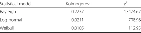
data are included in Section 4. Figure 1a shows the real sonar image without any object. Figure 1b presents the normalized amplitude distribution and the estimated distri-butions. As observed visually, the real background data is described by a Weibull distribution better than the other distributions. This is confirmed by the quantitative mea-sures presented in Table 1, according to the Kolmogorov distance and χ2criterion [21, 27]. As a consequence, the Weibull distribution, which lies between the two extremes of log-normal and Rayleigh, appears to be a good choice for modeling the background in multi-beam sonar image.

The statistics of the Weibull-distributed backgroundB

are described by the probability density function:

Fig. 1A comparison among different statistical models using a real sonar image.aA real sonar image without any object.bNormalized amplitude distribution and estimated distributions

Table 1Kolmogorov distance andχ2error by approximating the image of Fig. 1a

Statistical model Kolmogorov χ2

Rayleigh 0.2237 13474.67

Log-normal 0.0211 708.98

Weibull 0.0105 112.95

pBð Þ ¼B

wherekis the shape parameter andλis the scale

param-eter. Ther‐th order origin moment is defined as:

mB rð Þ¼λrΓ 1þr

k

ð2Þ

whereΓis the gamma function. The meanμBand

stand-ard deviationσBof the background are then given by:

μ_B ¼λΓ 1þ1

Setting the object amplitude A, the SNR can be de-fined as the ratio between the mean power of the object echo and the mean power of the background echo:

SNR¼20 log₁₀ jA−μBj

σB

ð5Þ

To investigate the local property, HOS is estimated within an image using a sliding computational window, and αis denoted as the proportion of object within the compu-tational window. When α= 0, the sliding computational window is totally composed of the background. The r‐th order origin moment computed within the whole window

mW(r)is defined [20] as:

mW rð Þ¼αmO rð Þþð1−αÞmB rð Þ ð6Þ

where mO(r) is r‐th order origin moment computed

within the object region. ThemO(r)is

mO rð Þ¼Ar ð7Þ

Derived from the third moment, the skewness com-puted on the computational window is given by:

SW ¼mWð Þ3

′

m′3_W=2_{ð Þ2} ð8Þ

where m′_{W r}ð Þ isr‐th order central moment. The relations

between the origin moment and central moment for 2‐th

and 3‐th are

λ. Substituting Eq. (5) into Eq. (11), the object amplitude

Acan be replaced by SNR. Thus, the local skewnessSW

is a function depending onαas well as SNR.

3 Local higher-order statistics for object representation

3.1 Object modeling by local HOS

Let us consider a simulated sonar image with a back-ground that follows a Weibull distribution, with a size of 100 × 100 pixels. The scale parameter k= 6.67 and the shape parameter λ= 0.45 are estimated from the real dataset. The local skewness SW displayed in

Fig. 2a is a two-dimensional surface with respect to α and SNR. The local skewness function gets higher values when α is low and SNR is high, and lower values when α is high and SNR is around 0 dB. In the computational window, a zero SW indicates that

the tails on both sides of the mean balance out, which is the case for a symmetric distribution. Nega-tive SW indicates that the tail on the left side of the

probability density function is longer than the right side. Conversely, positive SW indicates that the tail on

the right side is longer than the left side. Therefore, a large SW can be regarded as a clue to the potential

object, which is disrupted to local background distri-bution. Along the SNR axis, the α corresponding to the maximal SW is denoted as α'. The SNR versus α'

is shown in Fig. 2b. As shown in Fig. 2b, α' = 0 when SNR is below 3 dB, α' = 0.005 when SNR is above 25 dB, and α' between 0.01 and 0.125 when SNR is between 3 and 25 dB.

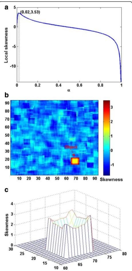
Given an object with SNR = 20 dB, the local skewness

SW versus α is shown in Fig. 3a. The local skewness

reaches the maximumSW= 3.53 withα= 0.02, and drops

as theαincreases. Modeling a square object SNR = 20 dB with the size TO= 3, local skewness is estimated using a

sliding computational window of size TW= 7. Note that

the units ofTO andTW are pixels throughout this paper.

A bias-corrected estimator of local skewnessSW[28] is

where n is the total pixel numbers of the image. In local skewness image, the object is represented by a square structure shown in Fig. 3b. The details of the square structure in local skewness image are shown in Fig. 3c, where the square structure is composed of lower values in the middle, higher values on the edge, and the highest value in the corners. The local skewness reaches the highest value ŜW= 3.48 corresponding to the case

that one single pixel of the object regions is included in the computational window, while the theoretical highest value is SW= 3.53. The special structure is due to the

variation ofαshown in Fig. 3a.

3.2 Representing the object with different SNR

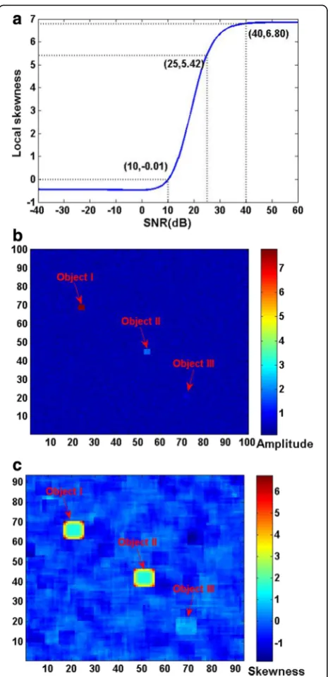
The ability of representing the object with different SNR is investigated by introducing object I SNR1= 40 dB,

ob-ject II SNR2= 25 dB, and object III SNR3= 10 dB to a

simulated image. The size of object isTO= 3 and the size

of computational window is TW= 7. The relations

be-tween the minimal proportion of object within the com-putational window αmin and the size of computational

windowTWcan be defined as:

αmin¼ 1

T2

W

ð13Þ

According to Eq. (13), TW= 7 derives αmin= 0.02. In

the case ofα= 0.02, the local skewnessSWversus SNR is

shown in Fig. 4a. The local skewness remains low value with SNR below 0 dB, and high value with SNR above 40 dB, but grows rapidly with SNR between 0 and 40 dB. In the simulated image shown in Fig. 4b, object I with high SNR is clear, object II with medium SNR is a bit

Fig. 2Local skewness function.aLocal skewness function ofαand SNR.bSNR versusα'

Fig. 3Local skewness for object representation (SNR = 20 dB).a Local skewness versusαwith SNR = 20 dB.bLocal skewness image. cThe details of object in local skewness

obscure, and object III with low SNR is totally mixed with the background. In the local skewness image shown in Fig. 4c, all objects are visually characterized by square structure. The higher the SNR, the larger the maximum value of the square structure and the more distinct the outline of the square structure is.

To evaluate the discrimination of the object between the original image and the local skewness image, the ob-ject contrast is defined as follows:

C¼ hT−μB0 A−μB

ð14Þ

wherehT is the maximum value of the square structure.

The mean and standard deviation of background in local

skewness image areμB'andσB':

Table 2 presents the performance of object representa-tion. The object with low SNR (SNR3= 10 dB) getsC=

5.0513, the object with medium SNR (SNR2= 25 dB)

gets C= 4.6754, and the object with high SNR (SNR3=

10 dB) getsC= 0.9650. In addition,hTfor all objects are

close to the theoretical values shown in Fig. 4a. Mapping from the original image to the local skewness image, an object with lower SNR achieves a higher C, whereas an object with higher SNR obtains a lowerCdue to the sat-uratedhT.

3.3 Choice of the computational window size

As suggested by the curve in Fig. 2b and Eq. (13), the αmin deriving from the size of computational window

TWshould correspond to theα' for a highesthT. For

ex-ample, an object with SNR = 10 dB, the suitable size of computational window is supposed to be TW= 3. In

order to confirm the assumption, a square object with a SNR of 10 dB and a size ofTO= 3 is inserted in a

simu-lated image shown in Fig. 5a, where the object is com-pletely unable to distinguish. The local skewness image with the size of computational window TW= 3,TW= 6,

and TW= 9 is shown in Fig. 5b–d, respectively. The

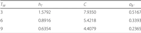
per-formance with different computational window sizes is presented in Table 3. The high hTand C are obtained

withTW= 3; however, the distinction between object and

background is obscure due to the high σB', as shown in

Fig. 5b. On the contrast, the low σB' is obtained with

TW= 9, but false alarms hinder the object determination

due to the low hTandC, as shown in Fig. 5d. With the

size of computational windowTW= 6, the local skewness

image shown in Fig. 5c provides satisfactory results with a compromise between the contrast Cand the standard deviationσB'.

Fig. 4Local skewness for multiple objects representation (R1= 40 dB, R2= 25 dB, andR3= 10 dB).aLocal skewness versus SNR withα= 0.02. bThe simulated image.cLocal skewness image

Table 2Performance of object representation (SNR1= 40 dB,

SNR2= 25 dB, and SNR3= 10 dB)

hT C σB'

SNR1 6.7473 0.9650 0.3072

SNR2 5.7620 4.6754 0.3072

Investigating the influences of the object size and shape, three objects (SNR = 20 dB) including square ob-ject I with the sizeTO= 3, square object II with the size

TO= 6, and sphere object III with the diameter TO= 8

are added into a simulated image shown in Fig. 6a. The local skewness image with the size of computational window TW= 4, TW= 7, and TW= 10 is shown in

Fig. 6b–d, respectively. One finds that the computational window sizeTW= 4,TW= 7, andTW= 10 is best for

de-scribing the structure of object size TO= 3, TO= 6, and

TO= 8, respectively. The performance reported in Table 4

confirms that the size of computational window TW= 7

corresponding to α= 0.02 obtains the highest C and moderateσB', which is considered the best result for the

case of SNR = 20 dB. It is concluded that a suitable window size, which is a bit larger than the object size, is able to rep-resent this object accurately and the outline of the sphere object can be described by the high values of the edges. However, the shape recognition needs to be further studied.

In conclusion, theαminderiving from the size of

com-putational windowTWshould correspond to theα' for a

highest hT; however, a trade-off between the highest

skewness of object hT and the standard deviation of

background σB' has to be made for selecting a suitable

computational window size. Moreover, the large window size generally makes it difficult to locate the object.

3.4 Side lobe suppression for object with high SNR

In the case of high SNR, an object can be observed visu-ally, but the image may be contaminated with high side lobes, which can occlude nearby objects. A side lobe suppression algorithm is required to make a reduction in the directions of arrival (DOA) of strong interfer-ences, while keeping the desired signal distortionless. Adaptive beamforming [29, 30], like the minimum-variance distortionless response (MVDR) beamformer [31], has shown good performance. However, a com-promise should be made between resolution and con-trast with limited computational cost. Therefore, we develop an algorithm based on background estimation, which identifies and offsets the high side lobes statisti-cally. Consider a sonar amplitude image X= {x(i,j)|1≤

i≤U, 1≤j≤V}, with a size ofU×Vpixels. The proposed algorithm comprises three main stages below and a de-scription of this algorithm in a pseudocode format is contained in Fig. 7.

(1) Calculate the normalized amplitude probability

distribution ofX, obtaining the max distribution

pointlmand the max inflection pointlV.

(2) Define_XVas the max points along the direction of

sampling number, from which the points larger

thanlVare labeled asXS.

(3) Save the object regions between the two valley

points around each point ofXS, calculate the

correction factordby the ratio between the max

side lobe peak_lsand the max pointlm, then

multiply the side lobe bydfor offsetting.

As an illustration, a real multi-beam sonar image con-taining a metal cube tied with ropes is displayed in

Fig. 5Local skewness for object representation with different sizes of computational window(R= 10 dB).aThe simulated image.bLocal skewness image withTW= 3.cLocal skewness image withTW= 6.dLocal skewness image withTW= 9

Table 3Performance of object representation with different computational window sizes (SNR = 10 dB)

TW hT C σB'

3 1.5792 7.9350 0.5167

6 0.8916 5.4218 0.3393

9 0.6354 4.4079 0.2365

Fig. 9a. The sonar amplitude image is shown in Fig. 8a, with the size of 1024 (beam number) × 350(sampling num-ber), and the corresponding normalized amplitude distribu-tion is presented in Fig. 8b. As shown in Fig. 8b, the max distribution pointlm= 0.62 and the max inflection pointlV

= 0.87 are obtained. The max amplitude for each sampling number is shown in Fig. 8c. As shown in Fig. 8c, the ampli-tude points XS, which are larger thanlV (dashed line),

in-cluding the highest points N (sampling number 250) are extracted from theXV. For each point belonging toXS, the

object regions are saved while the side lobe regions are off-set with the correction factor d. The object regions of N

(between two dashed lines) and the max side lobe peak are shown in Fig. 8d. Thels= 0.86 derives thed= 0.72.

Local skewness images before and after side lobe sup-pression are displayed in Fig. 9b, c, using the computa-tional window sizeTW= 14. The comparison reveals that

a considerable improvement for object representation has been achieved with the proposed algorithm. The side lobes are reduced and the object regions are retained with a square structure.

Another real multi-beam sonar image (shown in Fig. 12a) containing two groups of objects is used to

Fig. 6Local skewness for object representation with different sizes of computational window for three objects with different sizes and shapes. aThe simulated image.bLocal skewness image withTW= 4.cLocal skewness image withTW= 7.dLocal skewness image withTW= 10

Table 4Performance of object representation with different computational window sizes for three objects with different sizes and shapes (SNR = 20 dB)

TW C σB'

Object I Object II Object III

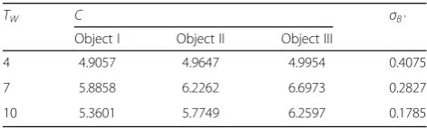
4 4.9057 4.9647 4.9954 0.4075

7 5.8858 6.2262 6.6973 0.2827

10 5.3601 5.7749 6.2597 0.1785

compare the algorithms’ performance. Figure 10a shows the side lobe suppression with MVDR beamformer, and Fig. 10b shows the side lobe suppression with back-ground estimation. It is clear that both the algorithms ad-equately reduce the side lobe. A significant SNR enhancement is achieved by the MVDR beamformer, whereas the boundary representations for potential objects are described in greater detail by the proposed algorithm.

Furthermore, the proposed algorithm is about 200 times faster than the MVDR beamformer. This is a significant improvement in terms of real-time performance.

4 Results and discussion

The proposed approach is verified on several real sonar images, which were obtained from multi-beam sonar de-veloped by Harbin Engineering University. The sonar covers a region of 140 (vertical) × 2.5 (horizontal), with

Fig. 8An illustration of side lobe suppression algorithm.aSonar amplitude image.bNormalized amplitude distribution.cThe max amplitude for each sampling number.dAmplitude of sampling number 250

Fig. 9The side-lobe suppression algorithm for a multi-beam sonar image.aOriginal image.bLocal skewness image before side lobe suppression.cLocal skewness image after side lobe suppression

an operating frequency of 300 kHz. The emitted signal is continuous wave (CW) with a pulse width of 0.1 ms, while the receiver is 64-element uniform linear array with a sampling frequency of 48 kHz. A large number of datasets collected during several trials are processed by beam forming and scan conversion methods [32–35], generating the image sequences with a resolution grid of 0.05 × 0.05 m2, and two of them are selected for example in the following.

Dataset I was acquired from a trial at an indoor tank, Harbin Engineering University, China. The correspond-ing image sequence I has the size of 111 × 241 pixels. Each frame describes the water-column scenes of 7 × 10 m2, in which a plastic ball and a metal block move to-gether in horizontal direction. Two typical frames are presented in Fig. 11a, b, where the objects are hardly vis-ible due to the small size and the similar amplitude of the object comparing to the background. The local skewness is estimated using the computational window size TW= 12, and the results are shown in Fig. 11c, d.

Both the objects are represented with the square struc-ture and distinguished from the background obviously. Table 5 gives the performance results, of which SNR ' is the SNR in local skewness image. The results show that local skewness image obtains the higher SNR ' and lower σB', in contrast to original image.

Dataset II was obtained from a trial at Songhua Lake, Jilin province, China. The corresponding image sequence II has the size of 361 × 601 pixels. Each frame describes the water-column scene of 20 × 30 m2, in which two groups of objects move relatively in vertical direction.

Fig. 10Side lobe suppression using different algorithms.aMVDR beamformer algorithm.bThe proposed algorithm

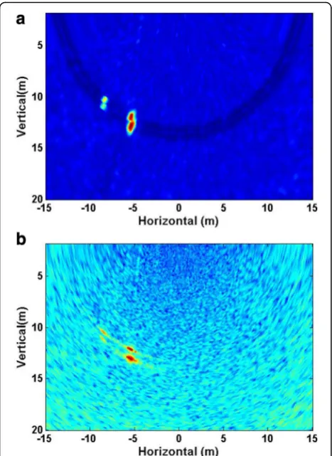
Each group of object is composed of a plastic ball and a metal block. A typical frame is displayed in Fig. 12a. Two groups of objects are distant, of which the object with low SNR can hardly be identified and the object with high SNR has high side lobes. Another frame is shown in Fig. 12b. Two groups of objects are close, of which the side lobes caused by highSNRobjects occlude the other objects. After side lobe suppression, the local skewness is estimated using the computational window size TW= 14. The results are presented in Fig. 12c, d,

where all objects are apparent with the square structure and the influence of side lobe are reduced. Table 6 gives the performance results. It shows that object 1 has a fluctuation of 11.87 dB between the original frames, whereas the corresponding fluctuation is only 1.99 dB between the local skewness frames. It confirms that local skewness is robust for object representation, especially in case of the object with a large SNR fluctuation be-tween consecutive frames. Furthermore, the boundary of the high SNR object is distinct by implementing the pro-posed side lobe suppression algorithm.

5 Conclusions

This paper investigates the capacity of local higher-order statistics (HOS) to represent objects in multi-beam sonar images. Local skewness is estimated using a sliding computational window applied to a sonar image, thus generating local skewness image of which a square struc-ture is associated with a potential object. One finds that: (1) The Weibull distribution has been proved to be a better choice for modeling the background of multi-beam sonar image, by comparing with the log-normal and Rayleigh distributions. (2) The square structure composes of lower values in the middle, higher values on the edge, and the highest value in the corners, and makes the object easily identifiable. (3) Mapping from original image to local skewness image, an object with lower SNR achieves a higher object contrast C, whereas an object with higher SNR obtains a lower object con-trast C, thus the robustness of object representation is improved, especially in case of the object with a large SNR fluctuation. (4) In order to select a suitable sliding computational window size, the αmin deriving from the

Fig. 12Local skewness for multiple objects representation in image sequence II.aFrame 1.bFrame 2.cLocal skewness for frame 1.dLocal skewness for frame 2

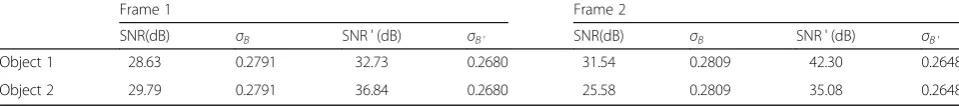
Table 5Performance comparisons between the original image and local skewness image for partial frames of image sequence I

Frame 1 Frame 2

SNR(dB) σB SNR ' (dB) σB' SNR(dB) σB SNR ' (dB) σB'

Object 1 28.63 0.2791 32.73 0.2680 31.54 0.2809 42.30 0.2648

Object 2 29.79 0.2791 36.84 0.2680 25.58 0.2809 35.08 0.2648

size of computational windowTW should correspond to

α' for a highest hT; however, a trade-off between the

higher skewness of objecthTand the lower standard

de-viation of backgroundσB'has to be made. (5) In the case

of object with high SNR, an algorithm based on back-ground estimation is able to significantly reduce the side lobe and completely retain object regions. The local HOS can provide the local feature relating to the poten-tial object for segmentation, detection and classification tasks; however, the robustness of local feature should be further tested and improved for shape recognition. In the future, we plan to extend this work to multiple ob-jects tracking in complex scenes.

Acknowledgements

This work was supported by the National Natural Science Foundation of China (Grant No. 41327004, 41376103, 41306038, and 41506115) and the Fundamental Research Funds for the Central Universities (Grant No. HEUCF160510). The authors would like to thank the anonymous reviewers for the constructive comments on the manuscript.

Competing interests

The authors declare that they have no competing interests.

Received: 16 June 2016 Accepted: 17 December 2016

References

1. SM Simmons, DR Parsons, JL Best, O Orfeo, SN Lane, R Kostaschuk, RJ Hardy, G West, C Malzone, J Marcus, P Pocwiardowski, Monitoring suspended sediment dynamics using MBES. J. Hydraul. Eng.136(1), 45_–49 (2010) 2. I Quidu, L Jaulin, A Bertholom, Y Dupas, Robust multitarget tracking in

forward-looking sonar image sequences using navigational data. IEEE J. Ocean. Eng.37(3), 417–430 (2012)

3. GG Acosta, SA Villar, Accumulated CA_–CFAR process in 2-D for online boject detection from sidescan sonar data. IEEE J. Ocean. Eng.40(3), 558–569 (2015)

4. XF Ye, ZH Zhang, PX Liu, HL Guan, Sonar image segmentation based on GMRF and level-set models. Ocean Eng.37(10), 891_–901 (2010)

5. T Celik, T Tjahjadi, A novel method for sidescan sonar image segmentation. IEEE J. Ocean. Eng.36(2), 186–194 (2011)

6. RJ Campbell, PJ Flynn, A survey of free-form object representation and recognition techniques. Comput. Vis. Image Underst.81(2), 166_–210 (2001) 7. B Moghaddam, A Pentland, Probabilistic visual learning for object

representation. IEEE Trans. Pattern Anal. Mach. Intell.19(7), 786–793 (2005) 8. D Dai, MJ Chantler, DM Lane, N Williams,Proceedings of International

Conference on Image Processing and Its Applications. A spatial-temporal approach for segmentation of moving and static objects in sector scan sonar image sequences, 1995, pp. 163–167

9. JP Stitt, RL Tutwiler, AS Lewis,Proceedings of the IASTED International Conference on Signal and Image Processing. Fuzzy c-means image segmentation of side-scan sonar images, 2001, pp. 27–32

10. M Mignotte, C Collet, P Perez, P Bouthemy, Sonar image segmentation using an unsupervised hierarchical MRF model. IEEE Trans. Image Process.

9(7), 1216–1231 (2000)

11. GJ Dobeck, JC Hyland, L Smedley,Proceedings of the International Society for Optical Engineering (SPIE). Automated detection/classification of sea mines in sonar imagery, 1997, pp. 90_–110

12. S Reed, Y Petillot, J Bell, Model-based approach to the detection and classification of mines in sidescan sonar. Appl Opt43(2), 237_–246 (2004) 13. DP Williams, Bayesian data fusion of multiview synthetic aperture sonar

imagery for seabed classification. IEEE Trans. Image Process.18(6), 1239– 1254 (2009)

14. CM Ciany, W Zurawski,Proceedings of Oceans Mts/IEEE Conference & Exhibition. Performance of computer aided detection/computer aided classification and data fusion algorithms for automated detection and classification of underwater mines, 2001, pp. 277_–284

15. S Reed, IT Ruiz, C Capus, Y Petillot, The fusion of large scale classified side-scan sonar image mosaics. IEEE Trans. Image Process.15(7), 2049_–2060 (2006) 16. GR Cutter Jr, Y Rzhanov, LA Mayer, Automated segmentation of seafloor

bathymetry from multibeam echosounder data using local Fourier histogram texture features. J. Exp. Mar. Biol. Ecol.285(2), 355–370 (2003) 17. A Mahiddine, J Seinturier, JM Boï, P Drap, D Merad,Proceedings of 20th

International Conference on Computer Graphics, Visualization and Computer Vision. Performances Analysis of Underwater Image Preprocessing Techniques on the Repeatability of SIFT and SURF Descriptors, 2012, pp. 275–282 18. S Lyu, H Farid, Steganalysis using higher-order image statistics. IEEE Trans.

Inf. Forensic Secur.1(1), 111_–119 (2006)

19. A Briassouli, I Kompatsiaris, Robust temporal activity templates using higher order statistics. IEEE Trans. Image Process.18(12), 2756_–2768 (2009) 20. F Maussang, J Chanussot, A Hetet, M Amate, Higher-order statistics for the

detection of small objects in a noisy background application on sonar imaging. EURASIP J. Adv. Signal Process.2007(1), 1–17 (2007) 21. F Maussang, J Chanussot, A Hetet, M Amate, Mean–standard deviation

representation of sonar images for echo detection: application to SAS images. IEEE J. Ocean. Eng.32(4), 956–970 (2007)

22. S Kuttikkad, R Chellappa,Proceedings of IEEE International Conference on Image Processing. Non-Gaussian CFAR techniques for target detection in high resolution SAR images, 1994, pp. 910_–914

23. JM Gelb, RE Heath, GL Tipple, Statistics of distinct clutter classes in midfrequency active sonar. IEEE J. Ocean. Eng.35(2), 220–229 (2010) 24. DA Abraham, JM Gelb, AW Oldag, Background and clutter mixture

distributions for active sonar statistics. IEEE J. Ocean. Eng.36(2), 231–247 (2011)

25. IR Joughin, DB Percival, DP Winebrenner, Maximum likelihood estimation of K distribution parameters for SAR data. IEEE Trans. Geosci. Remote Sens.

31(5), 989–999 (1993)

26. DR Iskander, AM Zoubir, B Boashash, A method for estimating the parameters of the K distribution. IEEE Trans. Signal Process47(4), 1147–1151 (1999)

27. M Mignotte, C Collet, P Pérez, P Bouthemy, Three-class Markovian segmentation of high-resolution sonar images. Comput.Vis.Image.Und76(3), 191–204 (1999)

28. DN Joanes, CA Gill, Comparing measures of sample skewness and kurtosis. J.R.Stat.Soc47(1), 183_–189 (1998)

29. JF Synnevag, A Austeng, S Holm, A low-complexity data-dependent beamformer. IEEE Trans. Ultrason. Ferroelectr. Freq. Control58(2), 281_–289 (2011) 30. CC Gaudes, I Santamaría, J Vía, EM Gómez, TS Paules, Robust array

beamforming with sidelobe control using support vector machines. IEEE Trans. Signal Process.55(2), 574–584 (2007)

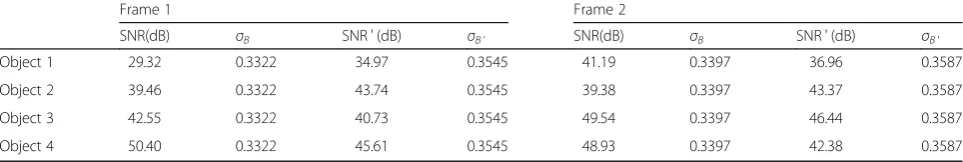
Table 6Performance comparisons between the original image and local skewness image for partial frames of image sequence II

Frame 1 Frame 2

SNR(dB) σB SNR ' (dB) σB' SNR(dB) σB SNR ' (dB) σB'

Object 1 29.32 0.3322 34.97 0.3545 41.19 0.3397 36.96 0.3587

Object 2 39.46 0.3322 43.74 0.3545 39.38 0.3397 43.37 0.3587

Object 3 42.55 0.3322 40.73 0.3545 49.54 0.3397 46.44 0.3587

31. M Wax, Y Anu, Performance analysis of the minimum variance beamformer. IEEE Trans. Signal Process44(4), 928_–937 (1996)

32. C Xu, HS Li, BW Chen, T Zhou, Multibeam interferometric seafloor imaging technology. J. Harbin Eng. Univ.34(9), 1159–1164 (2013)

33. X Liu, HS Li, T Zhou, C Xu, B Yao, Multibeam seafloor imaging technology based on the multiple sub-array detection method. J. Harbin Eng. Univ.

33(2), 197–202 (2012)

34. A Trucco, M Garofalo, S Repetto, G Vernazza, Processing and analysis of underwater acoustic images generated by mechanically scanned sonar systems. IEEE Trans. Instrum. Meas.58(7), 2061_–2071 (2009)

35. R Schettini, S Corchs, Underwater image processing: state of the art of restoration and image enhancement methods. EURASIP J. Adv. Signal Process.2010(3), 1–14 (2010)

Submit your manuscript to a

journal and benefi t from:

7 Convenient online submission 7 Rigorous peer review

7 Immediate publication on acceptance 7 Open access: articles freely available online 7 High visibility within the fi eld

7 Retaining the copyright to your article