R E S E A R C H
Open Access
On the robustness of set-membership
adaptive filtering algorithms
Hamed Yazdanpanah
*, Markus V. S. Lima and Paulo S. R. Diniz
Abstract
In this paper, we address the robustness, in the sense ofl2-stability, of the set-membership normalized least-mean-square (SM-NLMS) and the set-membership affine projection (SM-AP) algorithms. For the SM-NLMS algorithm, we demonstrate that it is robust regardless of the choice of its parameters and that the SM-NLMS enhances the parameter estimation in most of the iterations in which an update occurs, two advantages over the classical NLMS algorithm. Moreover, we also prove that if the noise bound is known, then we can set the SM-NLMS so that it never degrades the estimate. As for the SM-AP algorithm, we demonstrate that its robustness depends on a judicious choice of one of its parameters: the constraint vector (CV). We prove the existence of CVs satisfying the robustness condition, but practical choices remain unknown. We also demonstrate that both the SM-AP and SM-NLMS algorithms do not diverge, even when their parameters are selected naively, provided the additional noise is bounded. Numerical results that corroborate our analyses are presented.
Keywords: Adaptive filtering, Robustness, Set-theoretic estimation, Set-membership filtering, SM-NLMS, SM-AP
1 Introduction
The classical adaptive filtering algorithms are iterative estimation methods based on thepoint estimation theory [1]. This theory focuses on searching for a unique solution that minimizes (or maximizes) some objective function. Two widely used classical algorithms are the normalized least-mean-square (NLMS) and the affine projection (AP) algorithms. These algorithms present a trade-off between convergence rate and steady-state misadjustment, and their properties have been extensively studied [2, 3].
On the other hand, there are few adaptive filtering algo-rithms employing theset estimation theory[4]. This is the case of the algorithms following theset-membership filter-ing (SMF) paradigm. In set estimation theory, a setof feasible solutions is defined and any solution withinis equally acceptable. As real-world problems face many dif-ferent kinds of uncertainties (due to noise, quantization, interference, and modeling errors, for example), it makes more sense to search for an acceptable solution rather than trying to find a single/unique solution, as in point estimation theory.
*Correspondence: [email protected]
DEE–DEL/Poli & PEE/COPPE, Federal University of Rio de Janeiro, Rio de Janeiro, Brazil
The SMF combines the set estimation theory with data selection strategy to introduce the set-membership (SM) adaptive filtering algorithms [5]. The data selection is responsible for reducing the computational complexity of the SM algorithms, as their filter coefficients are updated only when the estimation error is larger than a prescribed upper bound, i.e., SM algorithms evaluate the innova-tion on the input data before incorporating them in the learning process [2, 5–7]. Two important SM algorithms are the membership NLMS (SM-NLMS) and the set-membership AP (SM-AP) algorithms, proposed in [8, 9], respectively. These algorithms keep the advantages of their classical counterparts, but they are more accurate, more robust against noise, and also reduce the compu-tational complexities due to the data selection strategy previously explained [2, 10–12]. Various applications of SM algorithms and their advantages over the classical algorithms have been discussed in the literature [13–21].
Despite the recognized advantages of the SM algo-rithms, they are not broadly used, probably due to the limited analysis of the properties of these algorithms. The steady-state mean-squared error (MSE) analysis of the SM-NLMS algorithm has been discussed in [22, 23]. Also, the steady-state MSE performance of the SM-AP algorithm has been analyzed in [10, 24, 25]. In addition,
the authors of the current paper have presented a few properties of the SM-NLMS algorithm in [26].
In this paper, the robustness of the SM-NLMS and the SM-AP algorithms are discussed in the sense ofl2
stabil-ity [3, 27]. Section 2 describes the robustness criterion. The robustness of the SM-NLMS algorithm is studied in Section 3, where we also discuss the cases in which the noise bound is assumed known and unknown. Section 4 presents the local and global robustness properties of the SM-AP algorithm with the details of the mathemati-cal manipulations left to appendices A and B. Section 5 contains the simulations and numerical results. Finally, concluding remarks are drawn in Section 6.
Notation:Scalars are denoted by lower-case letters. Col-umn vectors (matrices) are denoted by lowercase (upper-case) boldface letters. For a given iterationk, the optimum solution, the adaptive filter coefficient vector, the differ-ence between the optimal solution and the adaptive filter coefficient vector, and the input vector are denoted bywo, w(k), w˜(k), x(k) ∈ RN+1, respectively, whereN stands for the filter order. The desired signal, output signal, error signal, and noise signal are denoted by d(k), y(k), e(k), n(k) ∈ R, respectively. The output signal and the error signal are defined byy(k) xT(k)w(k)= wT(k)x(k)and e(k)d(k)−y(k), respectively, where the superscript(·)T stands for vector or matrix transposition. Thel2-norm of
a vectorw∈RN+1is denoted aswNk=0|w(k)|2.
2 Robustness criterion
At every iterationk, assume that the desired signald(k)is related to the unknown systemwoby
d(k)wTox(k) yo(k)
+n(k), (1)
wheren(k)denotes the unknown noise and accounts for both measurement noise and modeling uncertainties or errors. Also, we assume that the unknown noise sequence
{n(k)}has finite energy [3], i.e.,
j
k=0
|n(k)|2<∞, for allj. (2)
Suppose that we have a sequence of desired signals
{d(k)} and we intend to estimate yo(k) = wTox(k). For this purpose, assume thatyˆk|kis an estimate ofyo(k)and it is only dependent ond(j)forj = 0,· · ·,k. For a given positive number η, we aim at calculating the following estimates yˆk|k ∈ {ˆy0|0,yˆ1|1,· · ·,yˆN|N}, such that for any
n(k) satisfying (2) and any wo, the following criterion is satisfied:
j
k=0
ˆyk|k−yo(k)2
˜
wT(0)w˜(0)+j
k=0|n(k)|2 < η2,
for allj=0,· · ·,N (3)
where w˜(0) wo − w(0) andw(0) is our initial guess about wo. Note that the numerator is a measure of estimation-error energy up to iterationjand the denom-inator includes the energy of disturbance up to iteration j and the energy of the error w˜(0) that is due to the initial guess.
So, the criterion given in (3) requires that we adjust esti-mates {ˆyk|k} such that the ratio of the estimation-error energy (numerator) to the energy of the uncertainties (denominator) does not exceed η2. When this criterion is satisfied, we say that bounded disturbance energies induce bounded estimation-error energies, and therefore, the obtained estimates are robust. The interested reader can refer to [3], pages 719 and 720, for more details about this robustness criterion.
3 Robustness of the SM-NLMS algorithm
In this section, we discuss the robustness of the set-membership NLMS (SM-NLMS) algorithm. In subsec-tions 3.1 and 3.2, we briefly introduce the algorithm and present some robustness properties, respectively. We address the robustness of the SM-NLMS algorithm for the cases of unknown noise bound and known noise bound in subsections 3.3 and 3.4, respectively. Then, in subsection 3.5, we introduce a time-varying error bound aiming at achieving simultaneously fast conver-gence, low computational burden, and efficient use of the input data.
3.1 The SM-NLMS algorithm
The SM-NLMS algorithm is given by the following recur-sion [2]:
w(k+1)=w(k)+ μ(k)
x(k)2+δe(k)x(k), (4)
where
μ(k) 1−
¯
γ
|e(k)| if|e(k)|>γ¯,
0 otherwise, (5)
3.2 Robustness of the SM-NLMS algorithm
Let us consider the problem of identifying the unknown systemwo∈RN+1, such that
d(k)=wTox(k)+n(k), (6)
whered(k),n(k)∈Rdenote the desired (reference) signal and the additive measurement noise, respectively.
The following relation can be derived from (4):
˜
w(k+1)= ˜w(k)− μ(¯ k)
α(k)e(k)x(k)f(e(k),γ )¯ , (7) where w˜(k) wo − w(k) represents the discrepancy betweenw(k)and the quantity we aim to estimatewo, and
¯
μ(k),α(k), and the indicator functionf are defined as
¯
μ(k)1− γ¯
|e(k)|, (8)
α(k)x(k)2+δ, (9)
f(e(k),γ )¯
1 if|e(k)|>γ¯,
0 otherwise. (10)
In addition, observe that the error signal can be written as
e(k)=d(k)−wT(k)x(k)
=wTox(k)+n(k)−wT(k)x(k)
= ˜w T(k)x(k) ˜e(k)
+n(k), (11)
wheree˜(k)represents thenoiseless error, i.e., the error due to a mismatch betweenw(k)andwo.
By computing the energy of (7) and using (11), the robustness property given in Theorem 1 can be derived after some mathematical manipulations (refer to [26] for the proof ).
Theorem 1 (Local Robustness of SM-NLMS)For the SM-NLMS algorithm, it always holds that
˜w(k+1)2= ˜w(k)2,if f(e(k),γ )¯ =0 (12) or
˜w(k+1)2+μ(¯ k)
α(k)e˜
2(k)
< ˜w(k)2+μ(¯ k)
α(k)n
2(k), (13)
if f(e(k),γ )¯ =1.
Theorem 1 presents local bounds for the energy of the coefficient deviation when running from an iteration to the next one. Indeed, (12) states that the coefficient deviation does not change when no coefficient update is actually implemented, whereas (13) provides a bound for
˜w(k+1)2based on ˜w(k)2,˜e2(k), andn2(k), when an
update occurs. Using Theorem 1, Corollary 1 can be easily demonstrated (refer to [26] for the proof ).
Corollary 1(Global Robustness of SM-NLMS)For the SM-NLMS algorithm running from iteration 0 (initializa-tion) to a given iteration K, the following relation holds
˜w(K)2+ k∈Kup
¯
μ(k) α(k)e˜2(k)
˜w(0)2+ k∈Kup
¯
μ(k) α(k)n2(k)
<1, (14)
whereKup = ∅is the set containing the iteration indexes k in which w(k) is indeed updated. If Kup = ∅, then
˜w(K)2 = ˜w(0)2 due to (12), but this case is not of practical interest sinceKup = ∅means that no update is performed at all.
Corollary 1 states that, for the SM-NLMS algorithm, l2-stability from its uncertainties { ˜w(0),{n(k)}0≤k≤K} to its errors { ˜w(K),{˜e(k)}0≤k≤K} is invariably guaranteed.
Unlike the NLMS algorithm, in which the step-size parameter has to be selected properly to guarantee such l2-stability, for the SM-NLMS algorithm it is taken for
granted (i.e., no restriction is imposed onγ¯).
3.3 Convergence of{ ˜w(k)2}with unknown noise
bound
The robustness results mentioned in subsection 3.2 pro-vide bounds for the evolution of { ˜w(k)2} in terms
of other variables. However, we have experimentally observed that the SM-NLMS algorithm presents a well-behaved convergence of the sequence{ ˜w(k)2}, i.e., for most iterations we have ˜w(k+1)2 ≤ ˜w(k)2. There-fore, in this subsection, we investigate under which condi-tions the sequence{ ˜w(k)2}is (and is not) decreasing.
Corollary 2When an update occurs (i.e., f(e(k),γ )¯ =1),
˜
e2(k)≥n2(k)implies ˜w(k+1)2< ˜w(k)2.
ProofBy rearranging the terms in (13) we obtain
˜w(k+1)2+μ(¯ k)
α(k)
˜
e2(k)−n2(k)< ˜w(k)2, (15)
which is valid forf(e(k),γ )¯ = 1. Observe that μ(α(¯kk)) > 0 sinceα(k) ∈ R+andμ(¯ k) ∈ (0, 1)whenf(e(k),γ )¯ = 1. Thus μ(α(¯kk))˜e2(k)−n2(k) ≥ 0 whenf(e(k),γ )¯ = 1 and
˜
e2(k)≥n2(k). Therefore, when an update occurs,˜e2(k)≥ n2(k)⇒ ˜w(k+1)2< ˜w(k)2.
In words, Corollary 2 states that the SM-NLMS algo-rithm improves its estimatew(k+1)every time an update is required and the energy of the error signale2(k)is
dom-inated bye˜2(k), the component of the error which is due
Corollary 2 also explains why the SM-NLMS algorithm usually presents a monotonic decreasing sequence
{ ˜w(k)2}during its transient period. Indeed, in the early iterations, the absolute value of the error is generally large, thus |e(k)| > γ¯ ande˜2(k) > n2(k), implying that
˜w(k + 1)2 < ˜w(k)2. In addition, there are a few iterations during the transient period in which the input data do not bring enough innovation so that no update is performed, which means that ˜w(k+1)2= ˜w(k)2for these few iterations. As a conclusion, it is very likely to have ˜w(k+1)2≤ ˜w(k)2for all iterationskbelonging to the transient period.
After the transient period, however, the SM-NLMS algorithm may yield ˜w(k+1)2> ˜w(k)2in a few
iter-ations. Although it is hard to compute how often such an event occurs, we can provide an upper bound for the probability of this event as follows:
P ˜w(k+1)2> ˜w(k)2 the complementary error function [28], respectively. The first inequality follows from the fact that we do not know exactly what will happen with ˜w(k+1)2when an update
occurs ande˜2(k) <n2(k)at the same time1, and therefore, it corresponds to apessimistic bound. The second inequal-ity is trivial and the subsequent equalinequal-ity follows from [29] by parameterizingγ¯ asγ¯ = τσ2
n, whereτ ∈ R+ (typi-callyτ =5) and by modeling the errore(k)as a zero-mean Gaussian random variable with varianceσn2.
From (16), one can observe that the probability of obtaining ˜w(k+1)2 > ˜w(k)2is small. For instance,
meaning that the SM-NLMS algorithm uses the input data efficiently. Indeed, having ˜w(k+1)2> ˜w(k)2means that the input data was used to obtain an estimatew(k+1) which is further away from the quantity we aim to estimate wo, which is a waste of computational resources (it would be better not to update at all). Here, we showed that this rarely happens for the SM-NLMS algorithm, a property not shared by the classical algorithms, as it will be verified experimentally in Section 5.
3.4 Convergence of{ ˜w(k)2}with known noise bound In this subsection, we demonstrate that if the noise bound is known, then it is possible to set the threshold parameter
¯
γ of the SM-NLMS algorithm so that{ ˜w(k)2}is a
mono-tonic decreasing sequence. Theorem 2 and Corollary 3 address this issue.
Theorem 2 (Strong Local Robustness of SM-NLMS) Assume the noise is bounded by a known constant B∈R+, (i) and the maximum of (ii) as follows:
(i)e˜(k) >γ¯−n(k)⇒ ˜emin>γ¯−B≥B;
Corollary 3(Strong Global Robustness of SM-NLMS) Consider the SM-NLMS algorithm running from iteration 0 (initialization) to a given iteration K. Ifγ¯ ≥ 2B, then
˜w(K)2≤ ˜w(0)2, in which the equality holds only when
no update is performed along all the iterations.
The proof of Corollary 3 is omitted because it is a straightforward consequence of Theorem 2.
3.5 Time-varyingγ (¯ k)
After reading subsections 3.3 and 3.4, one might be tempted to setγ¯as a high value since it reduces the num-ber of updates, thus saving computational resources and also leading to a well-behaved sequence ˜w(k)2 that has high probability of being monotonously decreasing. However, a high value of γ¯ leads to slow convergence, because the updates during the learning stage (transient period) are less frequent and the step-sizeμ(k)is reduced as well. Hence,γ¯ represents a compromise between con-vergence speed and efficiency and therefore should be chosen carefully according to the specific characteristics of the application.
By using such aγ (¯ k), one obtains the best features of the high and low values ofγ¯ discussed in the first para-graph of this subsection. In addition, if the noise bound Bis known, then one should setγ (¯ k) ≥ 2Bfor allk dur-ing the steady-state, as explained in subsection 3.4. It is worth mentioning that (17) provides a general expression forτ(k) that allows it to vary smoothly along the itera-tions even within a single period (i.e., transient period or steady-state).
In order to apply theγ (¯ k)defined above, the algorithm should be able to monitor the environment to determine when there is a transition between transient and steady-state periods. An intuitive way to do this is to monitor the values of|e(k)|. In this case, one should form a win-dow with the E ∈ N most recent values of the error, compute the average of these |e(k)|within the window, and compare it against a threshold parameter to make the decision. An even more intuitive and efficient way to monitor the iterations relies on how often the algo-rithm is updating. In this case, one should form a window of lengthEcontaining Boolean variables (flags, i.e., 1-bit information) indicating the iterations in which an update was performed considering theE most recent iterations. Clearly, if many updates were performed within the win-dow, then the algorithm must be in the transient period; otherwise, the algorithm is likely to be in steady-state.
4 Robustness of the SM-AP algorithm
In this section, we address the robustness of the set-membership affine projection (SM-AP) algorithm. First, we introduce the SM-AP algorithm in subsection 4.1 and then we study its robustness properties in subsection 4.2. In subsection 4.3, we demonstrate that the SM-AP algo-rithm does not diverge.
4.1 The SM-AP algorithm
It is widely known that data-reusing algorithms can increase convergence speed significantly for correlated-input signals [2, 30, 31]. For this purpose, let us define the input matrixX(k), the error vectore(k), the desired vec-tord(k), the additive noise vectorn(k), and the constraint vector (CV)γ(k)as follows:
X(k)=[x(k)x(k−1) · · · x(k−L)]∈R(N+1)×(L+1),
e(k)=[e(k) (k−1)... (k−L)]T∈RL+1,
d(k)=[d(k)d(k−1) · · · d(k−L)]T∈RL+1,
n(k)=[n(k)n(k−1)...n(k−L)]T∈RL+1,
γ(k)=[γ0(k) γ1(k) · · · γL(k)]T∈RL+1,
(18)
where N is the order of the adaptive filter and L is the data-reusing factor, i.e.,Lprevious data are used together
with the data from the current iterationk. The error sig-nal is given bye(k) d(k)−XT(k)w(k), and the entries of the constraint vector should satisfy |γi(k)| ≤ ¯γ, for i = 0,. . .,L, whereγ¯ ∈ R+is the upper bound for the magnitude of the error signale(k).
The SM-AP algorithm is described by the following recursion [9]:
w(k+1)=
w(k)+X(k)A(k)(e(k)−γ(k)) if|e(k)|>γ¯,
w(k) otherwise, (19)
where we assume thatA(k)XT(k)X(k)−1∈RL+1×L+1
exists, i.e.,XT(k)X(k)is a full-rank matrix. Otherwise, we could add a regularization parameter as explained in [2].
4.2 Robustness of the SM-AP algorithm
Suppose that in a system identification problem the unknown system is denoted bywo∈RN+1and the desired (reference) vector is given by
d(k)XT(k)wo+n(k). (20)
By defining the coefficient mismatchw˜(k)wo−w(k), the error vector can be written as
e(k)=XT(k)wo+n(k)−XT(k)w(k)
=XT(k)w˜(k) e˜(k)
+n(k), (21)
where e˜(k) denotes the noiseless error vector (i.e., the error due to a nonzero w˜(k)). By defining the indicator functionf :R×R+→ {0, 1}as in (8) and using it in (19), the update rule of the SM-AP algorithm can be written as follows:
w(k+1)=w(k)
+X(k)A(k)(e(k)−γ(k))f(e(k),γ )¯ . (22) After subtractingwofrom both sides of (22), we obtain
˜
w(k+1)= ˜w(k)
−X(k)A(k)(e(k)− γ(k))f(e(k),γ )¯ . (23) Notice thatA(k)is a symmetric positive definite matrix. To simplify our notation, we will omit the indexkand the arguments of functionf that appear on the right-hand side (RHS) of the previous equation, then by decomposinge(k) as in (21) we obtain
˜
w(k+1)= ˜w−XAef˜ −XAnf+XAγf, (24)
from which Theorem 3 can be derived.
Theorem 3(Local Robustness of SM-AP) For the SM-AP algorithm, at every iteration we have
otherwise ⎧ ⎪ ⎪ ⎨ ⎪ ⎪ ⎩
˜w(k+1)2+˜eTAe˜
˜w(k)2+nTAn <1,if γTAγ <2γTAn
˜w(k+1)2+˜eTAe˜
˜w(k)2+nTAn =1,if γTAγ =2γTAn
˜w(k+1)2+˜eTAe˜
˜w(k)2+nTAn >1,if γTAγ >2γTAn
, (26)
where the iteration index k has been dropped for the sake of clarity, and we assume that ˜w(k)2+nTAn =0just to allow us to write the theorem in a compact form.
ProofProof is left to Appendix A.
The combination of the first two inequalities in (26), which corresponds to the case γTA γ ≤ 2 γTAn, has an interesting interpretation. It describes that for any constraint vectorγ satisfying this condition we have
˜w(k+1)2+ ˜eTAe˜≤ ˜w(k)2+nTAn, (27) no matter what the noise vector n(k) is. In this way, we can derive the global robustness property of the SM-AP algorithm.
Corollary 4 (Global Robustness of SM-AP) Suppose that the SM-AP algorithm running from 0 (initialization) to a given iteration K employs a constraint vector γ sat-isfying γTAγ ≤ 2γTAnat every iteration in which an update occurs. Then, it always holds that
˜w(K)2+ k∈Kup
˜
eTAe˜
˜w(0)2+ k∈Kup
nTAn ≤1, (28)
whereKup= ∅is the set comprised of the iteration indexes k in whichw(k)is indeed updated and the equality holds when γTAγ = 2 γTAn for every k ∈ Kup. If Kup =
∅, then ˜w(K)2 = ˜w(0)2, a case that has no practical interest since no update is performed.
ProofProof is left to Appendix B.
Observe that, unlike the SM-NLMS algorithm, the SM-AP algorithm requires the condition
γTAγ ≤ 2γTAnto be satisfied in order to guarantee l2-stability from its uncertainties { ˜w(0),{n(k)}0≤k≤K} to its errors { ˜w(K),{˜e(k)}0≤k≤K}. The next question is: are
there constraint vectors γ satisfying such a condition? This is a very interesting point because the LHS of the condition is always positive, whereas the RHS is not. Corollary 5 answers this question and shows an example of such a constraint vector.
Corollary 5 Suppose the CV is chosen asγ(k) = cn(k) in the SM-AP algorithm, where n(k) is the noise vector defined in(20). If0 ≤c ≤2, then the conditionγTAγ ≤
2γTAnalways holds, implying that the SM-AP algorithm is globally robust by Corollary 4.
Proof Substitutingγ(k) = cn(k) inγTAγ ≤ 2γTAn leads to the following condition(c2−2c)nT(k)A(k)n(k)≤ 0, which is satisfied forc2−2c≤0⇒0≤c≤2 sinceA(k) is positive definite. Hence, due to Corollary 4 the proposed
γ(k)leads to a globally robust SM-AP algorithm.
It is worth mentioning that the constraint vectorγ(k)in Corollary 5 is not practical becausen(k)is not observable. Therefore, Corollary 5 is actually related to the existence ofγ(k)satisfyingγTAγ <2γTAn.
Unlike the SM-NLMS algorithm, thel2-stability of the
SM-AP algorithm is not guaranteed. Indeed, as demon-strated in Theorem 3 and Corollary 4, a judicious choice of the CV is required for the SM-AP algorithm to be l2-stable.It is worth mentioning that practical choices of γ(k)satisfying the robustness conditionγTAγ ≤ 2γTAn for every iteration k are not known yet! Even widely used CVs, like the simple-choice CV [32], sometimes violate this condition as will be shown in Section 5. However, this does not mean that the SM-AP algorithm diverges. In fact, it does not diverge regardless the choice ofγ(k), as demonstrated in the next subsection.
4.3 The SM-AP algorithm does not diverge
When the SM-AP algorithm updates (i.e., when|e(k)|>γ¯), it generates w(k + 1) as the solution to the following optimization problem [2, 9]:
minimizew(k+1)−w(k)2
subject tod(k)−XT(k)w(k+1)=γ(k). (29)
The constraint essentially states that the a posteriori errors (k−l) d(k−l)−xT(k−l)w(k+1)are equal to their respectiveγl(k), which in turn are bounded byγ¯, as explained in subsection 4.1. This leads to the following derivation:
| (k−l)| = |d(k−l)−xT(k−l)w(k+1)| ≤ ¯γ,
|xT(k−l)w˜(k+1)+n(k−l)| ≤ ¯γ, (30) which should be valid for all iterations and suitable values of the involved variables. Therefore, we have
− ¯γ −n(k−l)≤xT(k−l)w˜(k+1)
≤ ¯γ −n(k−l). (31) Since the noise sequence is bounded and γ <¯ ∞, we have
−∞< N
i=0
xi(k−l)w˜i(k+1) <∞, (32)
| ˜wi(k+1)|is also bounded implying ˜w(k+1)2 < ∞, which means that the SM-AP algorithm does not diverge even when its CV is not properly chosen. In section 5 we verify this fact experimentally by using ageneral CV, i.e., a CV whose entries are randomly chosen but satisfying
|γi(k)| ≤ ¯γ. Such general CV leads to poor performance, in comparison to the SM-AP algorithm using adequate CVs, but the algorithm does not diverge.
The same reasoning could be applied to demonstrate that the SM-NLMS algorithm does not diverge as well. However, from Corollary 1, it is straightforward to verify that ˜w(K)2<∞for everyK, as the denominator in (14) is finite.
5 Simulations
In this section, we provide simulation results for the SM-NLMS and SM-AP algorithms in order to verify their robustness properties addressed in the previous sections. These results are obtained by applying the aforemen-tioned algorithms to a system identification problem. The unknown systemwois comprised of 10 coefficients drawn from a standard Gaussian distribution. The noisen(k)is a zero-mean white Gaussian noise with varianceσn2=0.01 yielding a signal-to-noise ratio (SNR) equal to 20 dB. The regularization factor and the initialization for the adap-tive filtering coefficient vector areδ= 10−12andw(0)= [ 0 · · · 0]T∈ R10, respectively. The error bound parame-ter is usually set asγ¯ =5σ2
n =0.2236, unless otherwise stated.
5.1 Confirming the results for the SM-NLMS algorithm
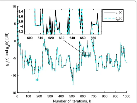
Here, the input signalx(k)is a zero-mean white Gaussian noise with variance equal to 1. Figure 1 aims at verify-ing Theorem 1. Thus, for the iterationskwith coefficient update, let us denote the left-hand side (LHS) and the
Number of iterations, k
0 0 5 1 0
0 0 1 0
0 5 0
g1
(k) and g
2
(k) [dB]
-25 -20 -15 -10 -5 0 5 10 15
g1(k)
g2(k)
1050 1100 1150 1200
-18 -17 -16 -15
Fig. 1Values ofg1(k)andg2(k)over the iterations for the SM-NLMS algorithm corroborating Theorem 1
right-hand side (RHS) of (13) asg1(k)andg2(k), respec-tively. In addition, to simultaneously account for (12), we define g1(k) = ˜w(k +1)2 andg2(k) = ˜w(k)2 for the iterations without coefficient update. Figure 1 depicts g1(k)andg2(k)considering the system identification sce-nario described in the beginning of Section 5. In this figure, we can observe thatg1(k)≤g2(k)for allk. Indeed, we verified thatg1(k) = g2(k) (i.e., curves are overlaid) only in the iterations without update, i.e., w(k +1) = w(k). In the remaining iterations, we haveg1(k) < g2(k), corroborating Theorem 1.
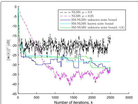
Figure 2 depicts the sequence ˜w(k)2 for the SM-NLMS algorithm and its classical counterpart, the SM-NLMS algorithm. For the SM-NLMS algorithm, we consider three cases: fixedγ¯with unknown noise bound (blue solid line), fixedγ¯ with known noise boundB = 0.11 (cyan solid line), and time-varyingγ (¯ k), defined as5σ2
n dur-ing the transient period and9σ2
nduring the steady-state, with unknown noise bound (green solid line). For the results using the time-varyingγ (¯ k), the window length is E=20 and when the number of updates in the window is less than 4, we assume the algorithm is in the steady-state period. For the NLMS algorithm, two different step-sizes are used:μ = 0.9, which leads to fast convergence but high misadjustment, andμ = 0.05, which leads to slow convergence but low misadjustment.
In Fig. 2, the blue curve confirms the discussion in Sub-section 3.3. Indeed, we can observe that the sequence
˜w(k)2represented by this blue curve increases only 30 times along the 2500 iterations, meaning that the SM-NLMS algorithm did not improve its estimatew(k+1) only in 30 iterations. Thus, in this experiment we have P ˜w(k+1)2> ˜w(k)2 = 0.012, whose value is lower than its corresponding upper bound given by erfc(√2.5)=0.0253, as explained in Subsection 3.3. Also,
Fig. 2 ˜w(k)2w
we can observe that the event ˜w(k+1)2 > ˜w(k)2
did not occur in the early iterations because in these iterationse˜2(k)is usually large due to a significant mis-match betweenw(k)andwo, i.e., the condition specified in Corollary 2 is frequently satisfied.
Also in Fig. 2, the cyan curve shows that when the noise bound is known we can obtain a monotonic decreasing sequence ˜w(k)2 by selecting γ¯ ≥ 2B, corroborat-ing Theorem 2 and Corollary 3. The sequence ˜w(k)2 represented by the green curve in Fig. 2 increases only 3 times, thus confirming the advantage of using a time-varying γ (¯ k) when the noise bound is unknown, as explained in Subsection 3.5. As compared to the SM-NLMS algorithm, the behavior of the sequence ˜w(k)2
for the NLMS algorithm is very irregular. Indeed, for the NLMS algorithm there are many iterations in which
˜w(k+1)2 > ˜w(k)2, even when using a small step-sizeμ. Hence, the NLMS algorithm does not use the input data as efficiently as the SM-NLMS algorithm does, given that the NLMS performs many “useless updates”.
In conclusion, an interesting advantage of the SM-NLMS algorithm over the SM-NLMS algorithm is that the former can achieve fast convergence and has a well-behaved sequence ˜w(k)2(which rarely increases) at the same time. In addition, the SM-NLMS algorithm also saves computational resources by not updating the filter coefficients at every iteration. In Fig. 2, the update rates of the blue, cyan, and green curves are 4.6, 1.5, and 1.9%, respectively. They confirm that the computational cost of the SM-NLMS algorithm is significantly lower than that of the NLMS algorithm2.
5.2 Confirming the results for the SM-AP algorithm
For the case of the SM-AP algorithm, the input is a first-order autoregressive signal generated asx(k)=0.95x(k− 1)+n(k−1). We test the SM-AP algorithm employing L = 2 (i.e., reuse of two previous input data) and three different constraint vectors (CVs)γ(k): a general CV, the simple choice CV, and the noise vector CV. The general CVγ(k), in which the entries are set asγl(k) = ¯γ for 0≤l≤L, illustrates a case where the CV is not properly chosen [5, 32]. The simple choice CV [5, 32] is defined as
γ0(k) = ¯γ|ee((kk))| andγl(k) = (k−l)for 1 ≤ l ≤ L. The noise vector CV is given byγ(k)=n(k).
The results depicted in Figs. 3, 4, 5, and 6 aim at ver-ifying Theorem 3 and Corollary 5. We define g1(k) and g2(k) as the numerator and the denominator of (26) in Theorem 3, respectively, when an update occurs; other-wise, we defineg1(k)= ˜w(k+1)2andg2(k)= ˜w(k)2. The results depicted in Fig. 3 illustrate that, for the general CV, there are many iterations in which g1(k) > g2(k) (about 293 out of 1000 iterations). This is an expected behavior since the general CV does not take into account (directly or indirectly) the value ofn(k)and,
Number of iterations, k
0 100 200 300 400 500 600 700 800 900 1000
g1
(k) and g
2
(k) [dB]
-15 -10 -5 0 5 10
g1(k)
g2(k)
600 610 620 630 640 650 660
-4.2 -4 -3.8 -3.6 -3.4
Fig. 3Values ofg1(k)andg2(k)over the iterations for the SM-AP algorithm withγ(k)as the general CV, whereg1(k)andg2(k)are the numerator and denominator of (26) in Theorem 3, when an update occurs; otherwise,g1(k)= ˜w(k+1)2andg2(k)= ˜w(k)2
therefore, it does not consider the robustness condition
γT(k)A(k)γ(k)≤2γT(k)A(k)n(k).
For the SM-AP algorithm employing the simple choice CV, however, there are very few iterations in which g1(k) >g2(k)(only 19 out of 1000 iterations), as shown in Fig. 4. This means that even the widely used simple choice CV does not lead to global robustness.
Figure 5 depicts the results for the SM-AP algorithm with γ(k) = n(k). In this case, we can observe that g1(k)≤g2(k)for allk, corroborating Corollary 5. In other words, this CV guarantees the global robustness of the SM-AP algorithm.
Number of iterations, k
0 100 200 300 400 500 600 700 800 900 1000
g1
(k) and g
2
(k) [dB]
-20 -15 -10 -5 0
g
1(k)
g2(k)
435 440 445 450 455 460 465
-17.2 -17 -16.8 -16.6 -16.4
Number of iterations, k
0 100 200 300 400 500 600 700 800 900 1000
g1
(k) and g
2
(k) [dB]
-40 -35 -30 -25 -20 -15 -10 -5 0
g1(k)
g2(k)
750 760 770 780
-30.5 -30 -29.5
Fig. 5Values ofg1(k)andg2(k)over the iterations for the SM-AP algorithm withγ(k)=n(k), whereg1(k)andg2(k)are the numerator and denominator of (26) in Theorem 3, when an update occurs; otherwise,g1(k)= ˜w(k+1)2andg2(k)= ˜w(k)2
Figure 6 illustratesg1(k)andg2(k)for the SM-AP algo-rithm with simple choice CV when the noise bound is known and 10 times smaller than γ¯. In contrast with the SM-NLMS algorithm, for the SM-AP algorithm even when the noise bound is known and much smaller thanγ¯, we cannot guarantee thatg1(k)≤g2(k)for allk. In Fig. 6, for example, we observeg1(k) >g2(k)in 15 iterations.
Figure 7 depicts the sequence ˜w(k)2for the AP and the SM-AP algorithms. For the AP algorithm, the step-size
μ is set as 0.9 and 0.05, whereas for the SM-AP algo-rithm the three previously defined CVs are tested. For the AP algorithm, we can observe an irregular behavior
Number of iterations, k
0 100 200 300 400 500 600 700 800 900 1000
g1
(k) and g
2
(k) [dB]
-14 -12 -10 -8 -6 -4 -2 0 2
g
1(k)
g2(k)
865 870 875 880
-12 -11 -10
Fig. 6Values ofg1(k)andg2(k)over the iterations for the SM-AP algorithm withγ(k)as the SC-CV when the noise bound is known, whereg1(k)andg2(k)are the numerator and denominator of (26) in Theorem 3, when an update occurs; otherwise,g1(k)= ˜w(k+1)2 andg2(k)= ˜w(k)2
Fig. 7 ˜w(k)2w(k)−w
o2for the AP and the SM-AP algorithms
of ˜w(k)2, i.e., this sequence increases and decreases very often. Even when a low value ofμis applied we still observe many iterations in which ˜w(k+1)2> ˜w(k)2 (425 out of 1000 iterations). The SM-AP algorithm using the general CV performs similar to the AP algorithm with highμ. But when the CV is properly chosen, like the sim-ple choice CV for examsim-ple, we observe that the number of iterations in which ˜w(k+1)2> ˜w(k)2is dramati-cally reduced (26 out of 1000 iterations), which means that the SM-AP with an adequate CV performs fewer “use-less updates” than the AP algorithm. Another interesting, although not practical, choice of CV isγ(k)=n(k), which leads to a monotonic decreasing sequence ˜w(k)2.
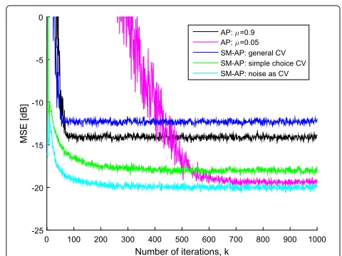
The MSE learning curves for the AP and the SM-AP algorithms are depicted in Fig. 8. These results were com-puted by averaging the squared error over 1000 trials for each curve. Observing the results of the AP algorithm, the
trade-off between convergence rate and steady-state MSE is evident. Indeed, excluding the SM-AP with general CV (which is not an adequate choice for the CV), the AP algo-rithm could not achieve fast convergence and low MSE simultaneously, as the SM-AP algorithm did.
In addition, observe thatγ(k) = n(k)leads to the best results in terms of convergence rate and steady-state MSE, but the performance of the SM-AP with simple choice CV is quite close. The average number of updates required by the SM-AP algorithm using the general CV, the simple choice CV, and the noise CV are 35, 9.7, and 3.6%, respec-tively, implying that the last two CVs also have lower computational cost. It is worth noticing that even when using the general CV, the SM-AP algorithm still converges although it presents poor performance, as explained in subsection 4.3.
6 Conclusions
In this paper, we addressed the robustness (in the sense of l2-stability) of the SM-NLMS and the SM-AP
algo-rithms. In addition to the already known advantages of the SM-NLMS algorithm over the NLMS algorithm, regard-ing accuracy and computational cost, in this paper we demonstrated that: (i) the SM-NLMS algorithm is robust regardless the choice of its parameters and (ii) the SM-NLMS algorithm uses the input data very efficiently, i.e., it rarely produces a worse estimate w(k +1) during its update process. For the case where the noise bound is known, we explained how to set properly the parame-terγ¯ so that the SM-NLMS algorithmnever generates a worse estimate, i.e., the sequence ˜w(k)2(the squared
Euclidean norm of the parameters deviation) becomes monotonously decreasing. For the case where the noise bound is unknown, we designed a time-varying parameter
¯
γ (k) that achieves simultaneously fast convergence and efficient use of the input data.
Unlike the SM-NLMS algorithm, we demonstrated that there exists a condition to guarantee the l2-stability of
the SM-AP algorithm. This robustness condition depends on a parameter known as the constraint vector (CV)
γ(k). We proved the existence of vectorsγ(k)satisfying such a condition, but practical choices remain unknown. In addition, it was shown that the SM-AP with an ade-quate CV uses the input data more efficiently than the AP algorithm.
We also demonstrated that both the AP and SM-NLMS algorithms do not diverge, even when their param-eters are not properly selected, provided the noise is bounded. Finally, numerical results that corroborate our study were presented.
Endnotes
1This is because Corollary 2 provides a sufficient, but
not necessary, condition for ˜w(k+1)2< ˜w(k)2.
2In comparison to the NLMS algorithm, whenever the
SM-NLMS algorithm updates it performs two additional operations: one division and one subtraction due to the computation of μ(k). However, for most of the itera-tions the SM-NLMS algorithm requires fewer operaitera-tions because it does not update often.
Appendix A: Proof of Theorem 3
For convenience, let us start by rewriting Eq. (24):
˜
w(k+1)= ˜w−XAef˜ −XAnf +XAγf. (33)
By computing the Euclidean norm of this equation and rearranging the terms, we get
˜w(k+1)2
= ˜wTw˜ − ˜wTXAef˜ − ˜wTXAnf
+ ˜wTXAγf − ˜eTATXTwf˜
+ ˜eTATA−1Aef˜ 2+ ˜eTATA−1Anf2
− ˜eTATA−1Aγf2−nTATXTwf˜
+nTATA−1Aef˜ 2+nTATA−1Anf2
−nTATA−1Aγf2+γTATXTwf˜
−γTATA−1Aef˜ 2−γTATA−1Anf2
+γTATA−1Aγf2
= ˜w2− ˜eTAef˜ − ˜eTAnf + ˜eTAγf
− ˜eTAef˜ + ˜eTAef˜ 2+ ˜eTAnf2
− ˜eTAγf2−nTAef˜ +nTAef˜ 2
+nTAnf2−nTAγf2+γTAef˜
−γTAef˜ 2−γTAnf2+γTAγf2, (34)
where it was used that A−1 = XT(k)X(k) and e˜(k) = XT(k)w˜(k). From the above equation, we observe that whenf =0 we have
˜w(k+1)2= ˜w(k)2 (35) as expected, sincef = 0 means that the algorithm does not update its coefficients. However, when f = 1 the following equality is achieved from (34):
˜w(k+1)2= ˜w2− ˜eTAe˜+nTAn
−2γTAn+γTAγ. (36) After rearranging the terms of the previous equation, we obtain
˜w(k+1)2+ ˜eTAe˜=
˜w2+nTAn−2γTAn+γTAγ . (37)
Therefore, ˜w(k+ 1)2 + ˜eTAe˜ < ˜w2+ nTAn if
γTAγ =2γTAn, and ˜w(k+1)2+˜eTAe˜> ˜w2+nTAn ifγTAγ >2γTAn.
Assuming ˜w2+nTAn = 0 we can summarize the discussion above in a compact form as follows:
⎧
Appendix B: Proof of Corollary 4
Denote byK{0, 1, 2,. . .,K−1}the set of all iterations. LetKup ⊆ Kbe the subset containing only the iterations
in which an update occurs, whereasKupc K \Kup is
comprised of the iterations in which the filter coefficients are not updated.
As a consequence of Theorem 3, when an update occurs the inequality given in (27) is valid providedγ is chosen such thatγTAγ ≤ 2γTAnis respected. In this way, by summing such inequality for allk∈Kupwe obtain
dent variable k, which we have omitted for the sake of simplification. In addition, for the iterations without coef-ficient update, we have (25), which can be summed for all k∈Kcupleading to both sides of the above inequality simplifying it as follows
˜w(K)2+
Assuming a nonzero denominator, we can write the previous inequality in a compact form
˜w(K)2+ is satisfied for every iteration in which an update occurs, i.e., for everyk ∈ Kup. The only assumption used in the
derivation is thatKup = ∅. Otherwise, we would have
˜w(K)2 = ˜w(0)2, which would occur only ifw(k)is never updated, which is not of practical interest.
Acknowledgements
The authors would like to thank CAPES, CNPq, and FAPERJ agencies for funding this research work.
Authors’ contributions
All authors have contributed equally. All authors read and approved the final manuscript.
Competing interests
The authors declare that they have no competing interests.
Publisher’s Note
Springer Nature remains neutral with regard to jurisdictional claims in published maps and institutional affiliations.
Received: 19 April 2017 Accepted: 8 October 2017
References
1. EL Lehmann, G Casella,Theory of Point Estimation, 2nd edn. (Springer, New York, 2003)
2. PSR Diniz,Adaptive Filtering: Algorithms and Practical Implementation, 4th edn. (Springer, New York, 2013)
3. AH Sayed,Adaptive Filters. (Wiley-IEEE, New York, 2008)
4. PL Combettes, The foundations of set theoretic estimation. Proc. IEEE. 81(2), 182–208 (1993). doi:10.1109/5.214546
5. MVS Lima, PSR Diniz, in21st European Signal Processing Conference (EUSIPCO 2013). Fast learning set theoretic estimation (IEEE, Marrakech, 2013), pp. 1–5
6. E Fogel, Y-F Huang, On the value of information in system
identification–bounded noise case. Automatica.18(2), 229–238 (1982). doi:10.1016/0005-1098(82)90110-8
7. JR Deller, Set-membership identification in digital signal processing. IEEE ASSP Magazine.6(4), 4–20 (1989). doi:10.1109/53.41661 8. S Gollamudi, S Nagaraj, S Kapoor, Y-F Huang, Set-membership filtering
and a set-membership normalized LMS algorithm with an adaptive step size. IEEE Signal Process. Lett.5(5), 111–114 (1998). doi:10.1109/97.668945 9. S Werner, PSR Diniz, Set-membership affine projection algorithm.
IEEE Signal Process. Lett.8(8), 231–235 (2001). doi:10.1109/97.935739 10. MVS Lima, PSR Diniz, Steady-state MSE performance of the
set-membership affine projection algorithm. Circ. Syst. Signal Process. 32(4), 1811–1837 (2013). DOI:10.1007/s00034-012-9545-4
11. R Arablouei, K Dogancay, inSignal&Information Processing Association Annual Summit and Conference (APSIPA ASC 2012). Tracking performance analysis of the set-membership NLMS adaptive filtering algorithm (IEEE, Hollywood, 2012), pp. 1–6
12. A Carini, GL Sicuranza, inIEEE International Conference on Acoustics, Speech and Signal Processing (ICASSP 2006). Analysis of a multichannel filtered-x set-membership affine projection algorithm, (2006).
doi:10.1109/ICASSP.2006.1660623
communications systems. IEEE Trans. Signal Process.46(9), 2372–2385 (1998). doi:10.1109/78.709523
14. S Nagaraj, S Gollamudi, S Kapoor, Y-F Huang, BEACON: An adaptive set-membership filtering technique with sparse updates. IEEE Trans. Signal Process.47(11), 2928–2941 (1999). doi:10.1109/78.796429 15. L Guo, Y-F Huang, Frequency-domain set-membership filtering and its
applications. IEEE Trans. Signal Process.55(4), 1326–1338 (2007). doi:10.1109/TSP.2006.888890
16. S Werner, Jr. JAA, PSR Diniz, Set-membership proportionate affine projection algorithms. EURASIP J. Audio Speech Music. Process.2007(1), 1–10 (2007). doi:10.1155/2007/34242
17. WA Martins, MVS Lima, PSR Diniz, inIEEE 9th Workshop on Signal Processing Advances in Wireless Communications (SPAWC 2008). Semi-blind data-selective equalizers for QAM, (Recife, Brazil, 2008), pp. 501–505. doi:10.1109/SPAWC.2008.4641658
18. H Yazdanpanah, PSR Diniz, New trinion and quaternion set-membership affine projection algorithms. IEEE Trans. Circ. Syst. II Express Briefs.64(2), 216–220 (2017)
19. MZA Bhotto, A Antoniou, Robust set-membership affine-projection adaptive-filtering algorithm. IEEE Trans. Signal Process.60(1), 73–81 (2012). doi:10.1109/TSP.2011.2170980
20. S Zhang, J Zhang, Set-membership NLMS algorithm with robust error bound. IEEE Trans. Circ. Syst. II Express Briefs.61(7), 536–540 (2014). doi:10.1109/TCSII.2014.2327376
21. WL Mao, Robust set-membership filtering techniques on gps sensor jamming mitigation. IEEE Sensors J.17(6), 1810–1818 (2017). doi:10.1109/JSEN.2016.2558192
22. MVS Lima, PSR Diniz, in7th International Symposium on Wireless Communication Systems (ISWCS 2010). On the steady-state MSE performance of the set-membership NLMS algorithm, (York, 2010), pp. 389–393. doi:10.1109/ISWCS.2010.5624323
23. N Takahashi, I Yamada, Steady-state mean-square performance analysis of a relaxed set-membership NLMS algorithm by the energy conservation argument. IEEE Trans. Signal Process.57(9), 3361–3372 (2009). doi:10.1109/TSP.2009.2020747
24. PSR Diniz, Convergence performance of the simplified set-membership affine projection algorithm. Circ. Syst. Signal Process.30(2), 439–462 (2011). doi:10.1007/s00034-010-9219-z
25. MVS Lima, PSR Diniz, inIEEE International Conference on Acoustics, Speech and Signal Processing (ICASSP 2010). Steady-state analysis of the set-membership affine projection algorithm, (Dallas, 2010), pp. 3802–3805. doi:10.1109/ICASSP.2010.5495836
26. H Yazdanpanah, MVS Lima, PSR Diniz, in9th IEEE Sensor Array and Multichannel Signal Processing Workshop (SAM 2016). On the robustness of the set-membership NLMS algorithm (IEEE, Rio de Janeiro, 2016) 27. M Rupp, Pseudo affine projection algorithms revisited: Robustness and
stability analysis. IEEE Trans. Signal Process.59(5), 2017–2023 (2011). doi:10.1109/TSP.2011.2113346
28. JG Proakis,Digital Communications. (McGraw-Hill, USA, 1995)
29. JF Galdino, JA Apolinario, MLR de Campos, inInternational Symposium on Circuits and Systems (ISCAS 2006). A set-membership NLMS algorithm with time-varying error bound, (2006), pp. 277–280
30. S Haykin,Adaptive Filter Theory, 4th edn. (Prentice Hall, Englewood Cliffs, 2002)
31. K Ozeki, T Umeda, An adaptive filtering algorithm using an orthogonal projection to an affine subspace and its properties. Electron. Commun. Jpn.67-A(5), 19–27 (1984)