Sparse and smooth canonical correlation analysis through rank 1 matrix approximation

R E S E A R C H

Open Access

Sparse and smooth canonical correlation

analysis through rank-1 matrix approximation

Abdeldjalil Aïssa-El-Bey

and Abd-Krim Seghouane

Abstract

Canonical correlation analysis (CCA) is a well-known technique used to characterize the relationship between two sets of multidimensional variables by finding linear combinations of variables with maximal correlation. Sparse CCA and smooth or regularized CCA are two widely used variants of CCA because of the improved interpretability of the former and the better performance of the later. So far, the cross-matrix product of the two sets of multidimensional variables has been widely used for the derivation of these variants. In this paper, two new algorithms for sparse CCA and smooth CCA are proposed. These algorithms differ from the existing ones in their derivation which is based on penalized rank-1 matrix approximation and the orthogonal projectors onto the space spanned by the two sets of multidimensional variables instead of the simple cross-matrix product. The performance and effectiveness of the proposed algorithms are tested on simulated experiments. On these results, it can be observed that they outperform the state of the art sparse CCA algorithms.

Keywords: Canonical correlation analysis, Sparse representation, Rank-1 matrix approximation

1 Introduction

Canonical correlation analysis (CCA) [1] is a multivariate analysis method, the aim of which is to identify and quan-tify the association between two sets of variables. The two sets of variables can be associated with a pair of linear transforms (projectors) such that the correlation between the projections of the variables in lower dimensional space through these linear transforms are mutually maximized. The pair of canonical projectors are easily obtained by solving a simple generalized eigenvalue decomposition problem, which only involves the covariance and cross-covariance matrices of the considered random vectors. CCA has been widely applied in many important fields, for instance, facial expression recognition [2, 3], detection of neural activity in functional magnetic resonance imag-ing (fMRI) [4, 5], machine learnimag-ing [6, 7] and blind source separation [8, 9].

In the context of high-dimensional data, there is usu-ally a large portion of features that is not informative in data analysis. When the canonical variables involve all fea-tures in the original space, the canonical projectors are, in

*Correspondence: [email protected]

1_{IMT Atlantique, UMR CNRS 6285 Lab-STICC, Université Bretagne Loire, Brest} 29238, France

Full list of author information is available at the end of the article

general, not sparse. Therefore, it is not easy to interpret canonical variables in such high-dimensional data anal-ysis. These problems may be tackled by selecting sparse subsets of variables, i.e. obtaining sparse canonical projec-tors in the linear combinations of variables of each data set [7, 10–12]. For example, in [11], the authors propose a new criterion for sparse CCA and applied a penalized matrix decomposition approach to solve the sparse CCA problem, and in [10], the presented sparse CCA approach computes the canonical projectors from primal and dual representations.

In this paper, we adopt an alternative formulation of the CCA problem which is based on rank-1 matrix approx-imation of the orthogonal projectors of data sets [13]. Based on this new formulation of the CCA problem, we developed a new sparse CCA based on penalized rank-1 matrix approximation which aims to overcome the draw-back of CCA in the context of high-dimensional data and improved interpretability. The proposed sparse CCA seeks to obtain iteratively a sparse pair of canonical pro-jectors by solving a penalized rank-1 matrix approxima-tion via a sparse coding method. Also, we present in this paper a smoothed version of the CCA problem based on rank-1 matrix approximation where we impose some smoothness on the projections of the variables in order to

avoid abrupt or sudden variations. These proposed algo-rithms differ from the existing ones in their derivation which is based on penalized rank-1 matrix approximation and the orthogonal projectors onto the space spanned by the two sets of multidimensional variables instead of the simple cross-matrix product [7, 10–12].

The rest of the paper is organized as follows: In Section 2, we give a brief review of the CCA problem. In Section 3, we present a formulation of CCA using a rank-1 matrix approximation of the orthogonal projectors of data sets and derive the smoothed solution. In Section 4, we introduce our new sparse CCA algorithm. In Section 5, we present some simulation results to demonstrate the effectiveness of the proposed method compared to state of the art CCA algorithms. Finally, Section 6 concludes the paper.

Henceforth, bold lower cases denote real-valued vectors and bold upper cases denote real-valued matrices. The transpose of a given matrixAis denoted byAT. All vectors will be column vectors unless transposed. Throughout the paper,Instands forn×nidentity matrix,0stands for the null vector and1nis the (column) vector ofRnwith one entries only. For a vectorx, the notationxiwill stand for theithcomponent ofx. As usual, for any integerm,1,m stands for{1, 2,. . .m}.

2 Canonical correlation analysis

In this section, we present briefly a review of CCA and its optimization problem. Let x ∈ Rdx _andy ∈ Rdy _be

the two random vectors, and we assume, without loss of generality, that bothxandyhave zero mean, i.e.E[x]=0 andE[y]=0whereE[·] is the expectation operator. CCA seeks a pair of linear transformwx ∈ Rdx andwy ∈ Rdy, such that correlation betweenwT_xxandwT_yyis maximized. Mathematically, the objective function to be maximized is given by:

Then, the objective functionρcan be rewritten as:

ρ(wx,wy)= invariant with the magnitude of the projection direction, we can turn to solve the following optimization problem

arg max

wx,wy

wT_xCxywy

subject to wT_xCxxwx=1, wTyCyywy=1.

Incorporating these two constraints, the Lagrangian is given by:

Taking derivatives with respect towxandwy, we obtain

∂J

These equations lead to the following generalized eigen-value problem

Cxywy = λCxxwx (6)

CT_xywx = λCyywy, (7)

whereλ=2λx=2λy. One way to solve this problem is as proposed in [6] by assumingCyyis invertible; we can write

wy= 1

λC−yy1CTxywx, (8)

and so substituting in Eq. (6) and assumingCxxis invert-ible gives

C−_xx1CxyC−yy1CTxywx=λ2wx. (9)

It has been shown in [6] that we can choose the associ-ated eigenvectors corresponding to the top eigenvalues of the generalized eigenvalue problem in (9) and then use (8) for find the correspondingwy. A number of existing meth-ods for sparse and smooth CCA have used the description provided above of CCA and focused on the use of the cross matrix Cxy for the derivation of new CCA variant algorithms [7, 10–12]. For the derivation of the proposed CCA variants, we adopt an alternative description of CCA which is based on the orthogonal projectors onto the space spanned by the two sets of multidimensional variables [13].

3 Canonical correlation analysis based on rank-1 matrix approximation

In practice, the covariance matrices Cxx, Cyy and Cxy are usually not available. Instead, the estimated covari-ance matrices are constructed based on given sample data set. LetX =[x1,. . .,xN]∈ Rdx×N andY =[y1,. . .,yN]∈ Rdy×N _{be the two sets of instances of x andy,}

respec-tively. Without loss of generality, we can assume both

μx = N−1

mization problem for CCA based on estimated covariance matrices is given by

arg max

wx,wy

wT_xXYTwy (10)

subject to wT_xXXTwx=1, wTyYYTwy=1,

and the generalized eigenvalue problem given by Eqs. (6) and (7) can be rewritten as

XYTwy = λXXTwx (11)

Y XTwx = λY YTwy. (12)

Then, by multiplying both sides of Eqs. (11) and (12) by

XT(XXT)−1andYT(Y YT)−1, respectively, we obtain: the orthogonal projectors onto the linear spans of the rows ofXandY respectively. So substitutingXTwxin Eq. (14) andYTwyin Eq. (13) gives

PxPyXTwx=KxyXTwx = λ2XTwx

PyPxYTwy=KyxYTwy = λ2YTwy.

Therefore, we can observe thatXTwxandYTwyare the left singular vectors associated to the largest singular val-ues of the matricesKxy =PxPyandKyx =PyPx respec-tively. By using the symmetric property of the matricesPx andPywe have:

Kyx=PyPx=PTyPTx =(PxPy)T=KTxy. (15)

The singular value decomposition of the matricesKxy andKyxis given by: (15) that the left singular vectors ofKyxcorrespond to the right singular vectors ofKxy.

In order to estimate the canonical projectors, we define the nearest rank-1 matrix approximation ofKxyby:

K1=d1u1vT1 ,

where the nearest means that the squared Frobenius norm betweenKxyandK1, defined byKxy−K12_F, is minimal.

Therefore, the rank-1 matrix approximation ofKxycan be formulated as solving the following optimization from:

arg min

wx,wy

Kxy−XTwxwTyY

2

F. (18)

Consequently, the projected dataXTwxandYTwy con-sist of the left and right singular vectors, respectively, associated to the largest singular value of the matrixKxy. Therefore, after estimating the left and right singular vec-torsu1andv1. respectively, and associated singular value

d1of the matrixKxy, we can obtain the projectorswxand wy by solving the following least square equations (see Step 5 in Algorithm 1):

arg min

Hence, for multiple projected data, the solution consist of the associated singular vectors corresponding to the top singular values of the matrixKxy.

Algorithm 1 Rank-1 matrix approximation CCA algorithm

From (18),we can observe that the optimization prob-lem (10) that involves the two constraints wT_xX2 = 1

andwT_yY2 =1 has now been transformed into a

rank-1 matrix approximation problem free of constraints and which can be solved with an SVD. With this approach, the proposed algorithm avoids the need of using these con-straints and hence also avoids their relaxations as it was proposed in [11].

One disadvantage of the above approach is the restric-tion thatXXTandY YTmust be non-singular. In order to prevent overfitting and avoid the singularity ofXXT and

γx > 0,γy > 0 are added in (10). Therefore, the regu-larized version solves the generalized eigenvalue problem withPx = XT(XXT +γxIdx)−

1_{X andP}

y = YT(Y YT +

γyIdy)−

1_{Y. We summarized the method of solving the}

entire rank-1 matrix approximation CCA in Algorithm 1.

3.1 Smoothed rank-1 matrix approximation CCA algorithm

In order to give preference to a particular solution with desirable properties for the proposed CCA problem, a regularization term (Tikhonov regularization) can be included in Eq. (18) such that:

arg min multiple of the identity matrix, giving preference to solu-tions with smaller norms. In our case, the matrices x andyare non-negative definite roughness penalty matri-ces used to penalize the second differenmatri-ces [14, 15], and

αx>0 andαy>0 are trade-off parameters such as:

The choice of such matrices may be used to enforce smoothness if the underlying vector is believed to be mostly continuous. The criterion of Eq. (19) can be rewrit-ten as

The optimization problem (21) can be alternatively solved by optimizingwx andwy. Specifically, we first fix wyand solvewxby minimizing (21). Then, we fixwxand minimize (21) to obtain wy. The above two procedures are repeated until convergence. Taking derivatives with respect towxandwy, we obtain

Therefore, we obtain wx and wy by solving the above equations in the least square sense (see Steps 7 and 9 in Algorithm 2). For multiple canonical projectors, let us consider the singular value decomposition ofKxy =

UDVT =

N i=1

diuivTi , where ui and vi are the ith

col-umn vectors of the matricesU andV, respectively, and

D = diag(d1,. . .,dN) such thatd1 ≥ d2 ≥ . . . ≥ dN. In order to estimate the second pair of canonical projec-tors, we must remove the contribution of the first pair of canonical projectors from the matrixKxy. To this end, we must remove the contribution of the singular vectors associated to the largest singular valued1using:

Kxy−d1u1vT1 =

N

i=2

diuivTi .

As presented in Section 3, the singular vectors u1

and v1 represent the projected data XTwx and YTwy, respectively. Then, by using the unitary property of matrices U and V, we can compute the singular value associated to the singular vectors u1 and v1 by d1 =

uT₁Kxyv1. Therefore, we propose to use a deflation

pro-cedure where the second pair of canonical projectors are defined by using the corresponding residual matrixKxy− wT_xXKxyYTwyXTwxwTyY. Then, we can define the other pair of projectors. The method for solving the smoothed rank-1 matrix approximation CCA is summarized by Algorithm 2.

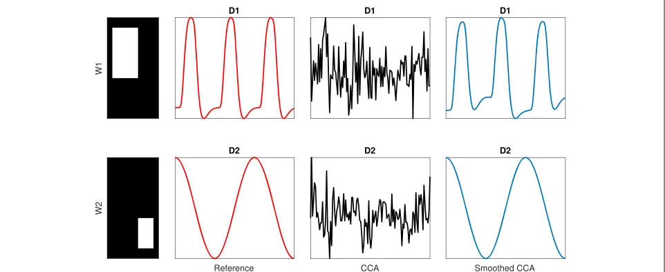
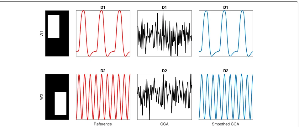
For illustrating the advantage of the proposed smoothed CCA approach over standard CCA, we generated for three distinct simulated activation cases; spatially independent case S1, partial spatial overlapS2, and complete spatial

overlap caseS3as done in [16]. Three temporal sources,

with 120 s duration, were constructed to represent the brain hemodynamics, i.e. block design activation (T1), and

two sinusoids (T2 andT3) with frequencies∈ {1.5, 9.5}

Hz, respectively, and box signals were used as brain acti-vation patterns [16]. Three distinct visual patterns of size 10×10 voxels were created with amplitudes of 1 at voxel indexes{2,. . ., 6} × {2,. . ., 6}for patternA,{8, 9} × {8, 9} for pattern B, and {5,. . ., 9} × {5,. . ., 9} for pattern C, and 0 elsewhere. The three simulated cases are shown in Figs. 1, 2 and 3: spatially independent events in Fig. 1, partial spatial overlapping events in Fig. 2 and complete spatial overlapping events in Fig. 3.

We can observe from Figs. 1, 2 and 3 that the proposed smoothed CCA algorithm have recovered both the tem-poral signal and spatial maps with better accuracy than CCA for the three presented casesS1,S2 andS3. This demonstrates the effectiveness of the proposed smoothed CCA approach in regularization when the estimated sig-nals are believed to be continuous and smooth.

4 Sparse CCA algorithm based on rank-1 matrix approximation

In this section, we will propose the sparse CCA method based on rank-1 matrix approximation by penalizing the optimization problem (18). Then, we propose an effi-cient iterative algorithm to solve the sparse solution of the proposed criterion.

In general, the canonical projectorswxandwyfound as solutions in Eq. (18) are not sparse, i.e., the entries of both

wx andwyare non-zeros. To obtain the sparse solution, we adopt the similar trick used in [7, 11, 12, 17] by impos-ing penalty functions on the optimization problem (18). Therefore, we can write the new optimization problem as:

arg min

wx,wy

_Kxy−XTwxwTyY

2

F subject to

Fx(wx)≤βx and Fy(wy)≤βy,

(22)

where Fx(·) andFy(·) are penalty functions, which can take on a variety of forms. Useful examples are0

-quasi-normF(z) = z0which count the non-zero entries of

a vector; Lasso penalty with1-norm F(z) = z1and

so on.

The optimization problem (22) can be alternatively solved by optimizingwxandwy. Specifically, we first fixwy and solve forwxby minimizing (22). Then, we fixwxand minimize (22) to obtainwy. The above two procedures are repeated until convergence.

The straightforward approach to solve this problem is to formulate it as an ordinary sparse coding task. Then, for a fixwy the problem (22) is equivalent to much simpler sparse coding problem

arg min

wx

KxyYTwy−XTwx2₂ subject to Fx(wx)≤βx,

which can be solved by using any sparse approximation method. In the same way, we can solve the problem (22) regarding wy for a fix wx by minimizing the following criterion:

arg min

wy

KT_xyXTwx−YTwy2₂ subject to Fy(wy)≤βy.

Based on the above description, we can obtain the first pair of sparse projectorswx andwy. For multiple projec-tion vectors, we propose to use a deflaprojec-tion procedure as

Fig. 2Illustrative example for simulated partial spatial overlap activation caseS2. Comparison of CCA and smoothed CCA (Algorithm 2) for simulated partial spatial overlap activation caseS2

presented in Section 3.1 where the second pair of sparse projectors are defined by using the corresponding residual matricesKxy−XTwxKxywTyY wTxXYTwy. Using the same way, we can define the other pair of sparse projectors.

The uncorrelated entries of the projected vector is obtained due to the orthogonality of the canonical com-ponents . The orthogonality among these comcom-ponents is lost due to the constraints added to the cost (18), a nice property enjoyed by standard CCA. Several other CCA procedures lose this property as well; this is just the price to pay for using the other constraints (sparsity or smoothness).

Then, we summarized the method of solving the entire sparse rank-1 matrix approximation CCA in Algorithm 3

In terms of difference between the proposed approach to achieve sparse CCA and the method proposed in [11]; the method proposed in [11] uses a penalized matrix decomposition on the cross-product matrixXYT

, whereas our proposed approach is based on a rank-1 matrix approximation ofKxy as defined in (18). Further-more, the method proposed in [11] makes the assumption thatXXTandY YTare identities to replace the constraints

wT_xXXTwx ≤ 1 andwTyY YTwy ≤ 1 bywx22 ≤ 1 and

wy2₂≤1 (Eqs. (4.2) and (4.3) of [11]). This assumption is

relaxed in the proposed sparse CCA algorithm presented in Section 4. This is obtained by directly including these constraintswT_xXXTwx = 1 andwTyY YTwy = 1 in the derivation of the matrixKxyused in the penalized rank-1 matrix approximation via Eq. (3).

The same argument is valid for [7] and [12] as both these papers are based on the cross-product matrixXYT; furthermore, their approaches used for regularization is similar to the one described in Algorithm 1 and therefore different from the regularization adopted in this paper given in Algorithm 2.

Algorithm 3 Sparse rank-1 matrix approximation CCA algorithm

In this section, we present several computer simulations in the context of blind channel estimation in single-input multiple-output (SIMO) systems and blind source sepa-ration to demonstrate the effectiveness of the proposed algorithm. We compare the performance of the proposed

algorithm with existing state of the art sparse CCA methods:

• The sparse CCA presented in [11], relying on a penalized matrix decomposition denoted PMD. An R package implementing this algorithm, called PMA, is available at http://cran.r-project.org/web/packages/ PMA/index.html. Sparsity parameters are selected using the permutation approach presented in [18] of which the code is provided in PMA package. • The sparse CCA presented in [7] where the CCA is

reformulated as a least-squares problem denoted LS CCA. A Matlab package implementing this algorithm is available at http://www.public.asu.edu/~jye02/ Software/CCA/.

• The sparse CCA presented in [12] where the sparse canonical projectors are computed by solving two

1-minimization problems by using the Linearized

Bregman iterative method [19]. This algorithm is denoted CCA LB (Linearized Bregman). We

re-implemented the sparse CCA algorithm proposed in [12] using Matlab.

For the proposed sparse CCA algorithm, we have used Fx(z) = Fy(z) = z0 as penalty functions. We solve

the sparse coding problem by using orthogonal matching pursuit (OMP) algorithm [20, 21]. For proposed smoothed CCA algorithm, we chosex=yand given by Eq. (20).

5.1 Synthetic data

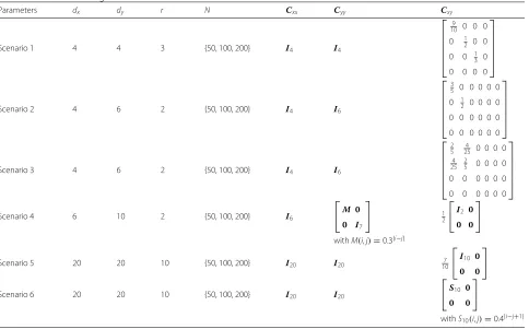
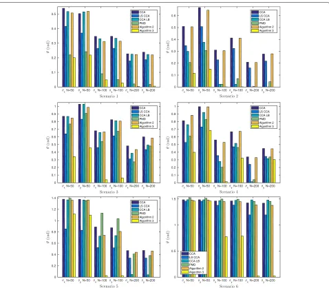
This simulation setup is inspired from [22]. The synthetic dataX andY were generating according to multivariate normal distribution, with covariance matrices described in Table 1. The number of simulations with each config-uration wasNk =1000. We compare the performance of our algorithm to the state of the art methods by estimating the precision accuracy of the space spanned by r esti-mated canonical projectors. We compute for each simula-tion runkthe angleθk(Wˆ k_x,Wx)between the subspace1 spanned by the estimated canonical projectors contained in the columns ofWˆ k and the subspace spanned by the true canonical projectors contained in the columns of

Table 1Simulation settings

For each algorithm, we used the following parameters: LS CCA algorithm withλx = λy = 0.5, CCA LB algo-rithm withμx = μy = 2; Algorithm 2 withαx = αy = 10−2; and Algorithm 3 with βx = βy = 3. The simu-lation performance on the estimated angle between the subspace spanned by the true canonical projectors and the estimated one by the different methods are reported in Tables 2 and 3, and plotted in Fig. 4. Note that the true canonical projectors Wx and Wy are sparse due to the structure of the matricesCxy(see Eqs. (8) and (9)).

We can observe that the simulation accuracy of the proposed sparse CCA method is significantly better com-pared to other CCA methods. In the case of low number of observations, the proposed sparse CCA method is still doing well and where the performance gain increases with increasing number of observations. This demonstrates the robustness of our sparse CCA method with respect to the number of available observations and the benefit of using our sparse CCA method in the context of a relatively low number of observations

5.2 Blind channel identification for SIMO systems Blind channel identification is a fundamental signal processing technology aimed at retrieving a system’s unknown information from its outputs only. Estimation of sparse long channels (i.e. channels with small number of nonzero coefficients but a large span of delays) is

considered in this simulation. Such sparse channels are encountered in many communication applications: high-definition television (HDTV) [23], underwater acous-tic communications [24] and wireless communications [25, 26]. The problem addressed in this section is to deter-mine the sparse impulse response of a SIMO system in a blind way, i.e. only the observed system outputs are avail-able and used without assuming knowledge of the specific input signal.

Let us consider a mathematical model where the input and the output are discrete, the system is driven by a single-input sequence s(t) and yields two output sequences x1(t) and x2(t) and the system has finite

impulse responses (FIR’s) hi(t), for t = 0,. . .,L and i = 1, 2 with L as the maximal channel length (which is assumed to be known). Such a system model can be described as follows :

x1(t) = s(t)∗h1(t) + η1(t)

x2(t) = s(t)∗h2(t) + η2(t), (23)

where∗denotes linear convolution,η(t) =[η1(t),η2(t)]T

is an additive spatial white Gaussian noise, i.e.

E[η(t)η(t)T_{]= σ}2_I

2 , and h =[hT1hT2]T with

Table 2Simulation results part 1

θx(rad) θy(rad) θx(rad) θy(rad) θx(rad) θy(rad)

Method N=50 N=100 N=200

Scenario 1: CCA 0.5395 0.5033 0.3468 0.3475 0.2273 0.2388

LS CCA 0.4161 0.3697 0.2649 0.2650 0.1784 0.1872

CCA LB 0.5172 0.5151 0.3310 0.3341 0.2250 0.2228

PMD 0.2203 0.2420 0.0908 0.0506 0.0207 0.0175

Algorithm 2 0.5074 0.5189 0.3123 0.3140 0.2225 0.2202

Algorithm 3 0.2011 0.2191 0.0491 0.0273 0.0044 0.0057

Scenario 2: CCA 0.5091 0.6682 0.3108 0.4123 0.2089 0.2771

LS CCA 0.3481 0.5083 0.2285 0.3247 0.1605 0.2182

CCA LB 0.3000 0.3761 0.0227 0.0228 0.0008 0.0009

PMD 0.2061 0.3068 0.0230 0.0706 0.0043 0.0443

Algorithm 2 0.5064 0.6462 0.3062 0.4111 0.2061 0.2792

Algorithm 3 0.1162 0.1508 0.0012 0.0015 0.0001 0.0001

Scenario 3: CCA 0.8699 1.0281 0.6800 0.8254 0.4823 0.6009

LS CCA 0.6398 0.8314 0.4608 0.6139 0.3116 0.4348

CCA LB 0.8681 1.0285 0.6575 0.8122 0.3859 0.4938

PMD 0.7690 0.9080 0.5382 0.6736 0.2736 0.4811

Algorithm 2 0.8465 0.9876 0.6654 0.8078 0.4345 0.5839

Algorithm 3 0.3424 0.4571 0.0393 0.0628 0.0001 0.0016

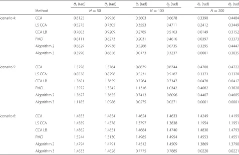
Table 3Simulation results part 2

θx(rad) θy(rad) θx(rad) θy(rad) θx(rad) θy(rad)

Method N=50 N=100 N=200

Scenario 4: CCA 0.8125 0.9956 0.5603 0.6678 0.3390 0.4484

LS CCA 0.5275 0.7305 0.3553 0.4711 0.2412 0.3449

CCA LB 0.7603 0.9209 0.2785 0.5163 0.0149 0.3152

PMD 0.6111 0.8273 0.2031 0.4616 0.0397 0.3373

Algorithm 2 0.8829 0.9938 0.5288 0.6735 0.3295 0.4447

Algorithm 3 0.3990 0.6856 0.0173 0.3237 0.0001 0.3035

Scenario 5: CCA 1.3798 1.3764 0.8879 0.8744 0.4700 0.4722

LS CCA 0.8538 0.8298 0.5231 0.5187 0.3373 0.3378

CCA LB 1.3681 1.3659 0.7264 0.7347 0.0478 0.0417

PMD 1.3972 1.3542 1.1316 1.0342 0.4082 0.3820

Algorithm 2 1.3627 1.3655 0.7413 0.8096 0.4407 0.4605

Algorithm 3 1.1185 1.0986 0.0275 0.0271 0.0001 0.0001

Scenario 6: CCA 1.4853 1.4854 1.4624 1.4633 1.4249 1.4199

LS CCA 1.4589 1.4578 1.3797 1.3838 1.1954 1.1951

CCA LB 1.4862 1.4851 1.4684 1.4740 1.4830 1.4793

PMD 1.5244 1.5130 1.4985 1.4954 1.4553 1.4551

Algorithm 2 1.4794 1.4791 1.4512 1.4509 1.3869 1.3790

Fig. 4Synthetic data simulation results. Performance comparison of CCA, LS CCA, CCA LB, PMD, Algorithm 2 and Algorithm 3 for synthetic data

is to estimate the channel coefficients vector h. The identification method presented by Xu et al. in [27] which is closely related to linear prediction exploits the com-mutativity of the convolution. Based on this approach and inspired from [28], we present in the following an experience to asses the performance of blind channel identification methods based on CCA.

From Eq. (23), the noise-free outputsxi(n),i=1, 2 and using the commutativity of convolution, it follows :

h2(t)∗x1(t)=h1(t)∗x2(t). (24)

In case the outputsxi(t)are corrupted by additive noise, this property inspired the design of the identification dia-gram shown in Fig. 5, which allows to find estimates of the channels impulse response,h1 andh2, by collecting

T observations sample and minimizing the following cost function

arg min

h1,h2

X1h2−X2h12

subject to X1h12= X2h22=1 ,

where

Xi= ⎡ ⎢ ⎣

xi(L) . . . xi(0) ..

. . .. ... xi(T−1) . . . xi(T−L−1)

⎤ ⎥

⎦ i=1, 2.

This problem is a canonical correlation analysis (CCA) problem.

Fig. 5SIMO system scheme. The block diagram of a SIMO system A linear SIMO system and the corresponding blind identification diagram

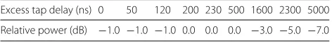
polynomial transfer function of degreeL = 66. The chan-nel impulse response is generated following 3GPP ETU (Extended Typical Urban) channel model [29] with fre-quency sampling 15.36 MHz which is used to model a channel impulse response for urban area in the context of wireless communications. The multipath delay profile for this channel is shown in Table 4.

The input signal is a BPSK i.i.d. sequence of length T = {256, 1024}. The observation is corrupted by the additive white Gaussian noise with a varianceσ2_chosen

such that the signal to noise ratio SNR= _σh₂2 varies in the range [ 0, 40] in dB. Statistics are evaluated overNk=100 Monte Carlo runs, and estimation performance are given by the normalized mean square error criterion :

NMSE= 1

wherehkdenotes the estimated channel coefficient vector at thekth_{Monte Carlo run. For each algorithm, we used} the following parameters: LS CCA algorithm withλx =

λy = 10−2, CCA LB algorithm with μx = μy = 10−1; Algorithm 2 withαx=αy =10−3; and Algorithm 3 with

βx=βy=10.

In Figs. 6 and 7, the normalized mean square error is plotted versus the SNR for the proposed approaches and state of the art algorithm. It is clearly shown that our sparse CCA based on rank-1 matrix approximation provide the best results for all SNR range and all observa-tion length. Especially, we can observe that the proposed method outperforms the PMD algorithm [11] by 9 dB for moderate and high SNR. This results show the robustness of the proposed method against the additive noise and its fast convergence. Indeed, from Fig. 6, we can observe that the proposed sparse CCA method provide for moder-ate and high SNR a near-optimal performance even in the case of low observation size.

Table 43GPP extended typical urban channel model [29]

Excess tap delay (ns) 0 50 120 200 230 500 1600 2300 5000

Relative power (dB) −1.0 −1.0 −1.0 0.0 0.0 0.0 −3.0 −5.0 −7.0

Fig. 6NMSE versus SNR forT=256. Normalized mean square error (NMSE) versus the SNR for SIMO system with two sensors and

T=256: performance comparison between CCA based methods for blind channel identification

5.3 Blind source separation for fMRI signals

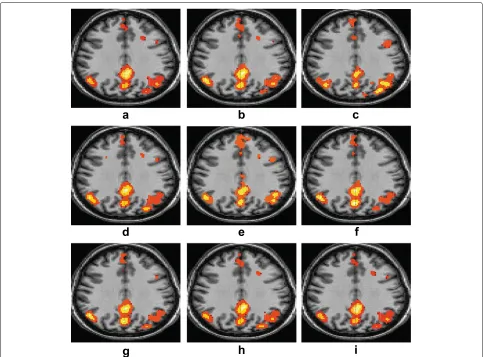
In this section, we evaluate the performance of the pro-posed CCA variant algorithms on a problem of func-tional magnetic resonance imaging (fMRI) resting state experiment (see Fig. 8 and Table 5). In this case, we are interested in functional connectivity and recovering a resting state network, i.e. the default mode network from a data matrix Y formed by vectorizing each time series observed in every voxel creating a matrixn×Nwheren is the number of time points andNthe number of voxels (≈10, 000−100, 000) [30].

Fig. 7NMSE versus SNR forT₌1024. Normalized mean square error (NMSE) versus the SNR for SIMO system with two sensors and

Fig. 8FMRI simulation results. The functional connectivity results of a single subject for default mode network (DMN) using eight different CCA variant algorithms.aReference.bCCA.cLS CCA,_λx=λy=0.5.dCCA LB,μx=μy=10.ePMD,fAlgorithm 2,αx=αy=10−4.gAlgorithm 2, αx=αy=10−3.hAlgorithm 3,βx=βy=3.iAlgorithm 3,βx=βy=4

To use CCA, either a second data set obtained from a different subject is used or the second data set is obtained from the original data Y by time delay [31]. This last option is used in this application example. Instead of tak-ing N as the total number of voxels, only the cortical, subcortical and cerebellum regions in the brain obtained by parcellating the whole brain into 116 ROIs using auto-mated anatomical labelling [32] were considered. For each considered region, the average time series was generated and used.

The single subject (id 100307) rsfMRI dataset used in this section was obtained from the Human Connectome Project Q1 release [33]. The acquisition parameters of rsfMRI data are 90 × 104 matrix, 220 mm FOV, 72

slices, TR = 0.72 s, TE = 33.1 ms, flip angle = 52◦ , BW = 2290Hz/Px, in-plane FOV = 208 × 180 mm with 2.0 mm isotropic voxels. The obtained data was already preprocessed with the preprocessing pipeline consisting of motion correction, temporal pre-whitening, slice time correction and global drift removal, and the scans were spatially normalized to a standard MNI152 template and were resampled to 2 mm × 2 mm × 2 mm voxels. The reader is referred to [33, 34] for more details regarding data acquisition and preprocessing.

The second data set obtained by a single sample delay was used for CCA. The different CCA algorithms were applied onY andYt−1of dimensionn×Nto allow us to

generate canonical correlation components representing

Table 5Performance comparison in terms of correlation with the reference Fig. 8 (a)

Algorithms CCA LS CCA CCA LB PMD Algo 2 (f) Algo 2 (g) Algo 3 (h) Algo 3 (i)

maximally correlated temporal profile. The neural dynam-ics of interest can be obtained by correlating the mod-ulation profile of the canonical correlation components with the time series representing average neural dynamics for regions of interest (ROIs). For functional connectiv-ity analysis of the default mode network (DMN), the modulation profile that was most correlated with pos-terior cingulate cortex (PCC) representative time series is used. Using the neural dynamics of interest, sparsely distributed and clustered origin of the dynamics are obtained by converting the associated coefficient rows to z-scores.

Using the different CCA variant algorithms, the con-nected regions obtained for DMN are mostly PCC, medial pre-frontal cortex (MFC) and right inferior parietal lobe (IPL). As there is no gold standard reference for DMN connectivity available, therefore, we relied on the simi-larity of temporal dynamics of DMN-based modulation profile with PCC representative time series. The similar-ity measure used was correlation and estimated as> 0.9 for all the algorithms.

6 Conclusions

In this paper, we have developed two new variants of CCA; more specifically, we have introduced new algorithms for sparse and smooth CCA. The proposed algorithms are based on penalized rank-1 matrix approximation and dif-fer from the existing ones in the matrices they use for their derivation. Indeed, instead of focusing on the cross-matrix product of the two sets of multidimensional variables, we have used the product of the orthogonal projectors onto the space spanned by the columns of the two sets of mul-tidimensional variables. Using this approach, the sparse and smooth CCA algorithms proposed differ only in the penalty used in the penalized rank-1 matrix approxima-tion. Simulation results illustrating the effectiveness of the proposed CCA variant algorithms are provided where we can observe that proposed sparse CCA outperforms state of the art methods. As a continuation of the pre-sented work and in order to fix the tuning parameters of the proposed approaches, the main idea of the per-mutation method presented in [18] will be studied and adapted.

Endnotes

1_{LetAandBbe two matrices. In order to compute the}

angleθbetween the subspaces spanned by the columns of

AandB; first, we compute an orthonormal basisA_⊥and

B_⊥for the range ofAandBrespectively.θis computed by

θ =arccos(min(AT_⊥B_⊥)).

Funding

No funding was received or used to prepare this manuscript.

Authors’ contributions

All authors contributed equally to this work. All authors discussed the results and implications and commented on the manuscript at all stages. Both authors read and approved the final manuscript.

Competing interests

The authors declare that they have no competing interests.

Author details

1_{IMT Atlantique, UMR CNRS 6285 Lab-STICC, Université Bretagne Loire, Brest}

29238, France.2Department of Electrical and Electronic Engineering, University of Melbourne, Parkville, Melbourne 3010, Australia.

Received: 8 March 2016 Accepted: 24 February 2017

References

1. H Hotelling, Relations between two sets of variables. Biometrika.28(3–4), 321–377 (1936)

2. W Zheng, X Zhou, C Zou, L Zhao, Facial expression recognition using kernel canonical correlation analysis (KCCA). IEEE Trans. Neural Netw.

17(1), 233–238 (2006)

3. XY Jing, S Li, C Lan, D Zhang, J Yang, Q Liu, Color image canonical correlation analysis for face feature extraction and recognition. Signal Process.91(8), 2132–2140 (2011)

4. O Friman, J Carlsson, P Lundberg, M Borga, H Knutsson, Detection of neural activity in functional MRI using canonical correlation analysis. Magn. Reson. Med.45(2), 323–330 (2001)

5. DR Hardoon, J Mourao-Miranda, M Brammer, J Shawe-Taylor, Unsupervised analysis of fMRI data using kernel canonical correlation. NeuroImage.37(4), 1250–1259 (2007)

6. DR Hardoon, S Szedmak, J Shawe-Taylor, Canonical correlation analysis: an overview with application to learning methods. Neural Comput.

16(12), 2639–2664 (2004)

7. L Sun, S Ji, J Ye, Canonical correlation analysis for multilabel classification: a least-squares formulation, extensions, and analysis. IEEE Trans. Pattern Anal. Mach. Intell.33(1), 194–200 (2011)

8. W Liu, DP Mandic, A Cichocki, Analysis and online realization of the CCA approach for blind source separation. IEEE Trans. Neural Netw.18(5), 1505–1510 (2007)

9. Y-O Li, T Adali, W Wang, VD Calhoun, Joint blind source separation by multiset canonical correlation analysis. IEEE Trans. Signal Process.57(10), 3918–3929 (2009)

10. DR Hardoon, J Shawe-Taylor, Sparse canonical correlation analysis. Mach. Learn.83(3), 331–353 (2011). doi:10.1007/s10994-010-5222-7

11. DM Witten, R Tibshirani, T Hastie, A penalized matrix decomposition, with applications to sparse principal components and canonical correlation analysis. Biostatistics.10(3), 515–534 (2009).

doi:10.1093/biostatistics/kxp008

12. D Chu, LZ Liao, MK Ng, X Zhang, Sparse canonical correlation analysis: new formulation and algorithm. IEEE Trans. Pattern Anal. Mach. Intell.

35(12), 3050–3065 (2013)

13. KV Mardia, JT Kent, JM Bibby,Multivariate Analysis. Probability and mathematical statistics, 1st edn. (Academic Press, University of Leeds, Leeds, 1979)

14. AN Tikhonov, On the stability of inverse problems. Doklady Akademii nauk SSSR.39(5), 195–198 (1943)

15. JO Ramsay, BW Silverman,Functional Data Analysis, 2nd edn. (Sprinver-Verlag, New York, 2005)

16. K Lee, SK Tak, JC Yee, A data driven sparse GLM for fMRI analysis using sparse dictionary learning and MDL criterion. IEEE Trans. Med. Imaging.

30, 1176–1089 (2011)

17. A Aïssa-El-Bey, A-K Seghouane, inIEEE International Conference on Acoustics, Speech and Signal Processing (ICASSP). Sparse canonical correlation analysis based on rank-1 matrix approximation and its application for FMRI signals, (2016), pp. 4678–4682.

doi:10.1109/ICASSP.2016.7472564

19. JF Cai, S Osher, Z Shen, Convergence of the linearized bregman iteration for1-norm minimization. Technical Report CAM Report 08–52, University

of California Los Angeles (2008)

20. YC Pati, R Rezaiifar, PS Krishnaprasad. Orthogonal matching pursuit: recursive function approximation with applications to wavelet decomposition, Proceedings of 27th Asilomar Conference on Signals, Systems and Computers, vol. 1, (Pacific Grove, 1993), pp. 40–44. doi:10.1109/ACSSC.1993.342465

21. G Davis, S Mallat, M Avellaneda, Adaptive greedy approximations. Constr. Approximation.13(1), 57–98 (1997). doi:10.1007/BF02678430

22. JA Branco, C Croux, P Filzmoser, MR Oliveira, Robust canonical correlations: a comparative study. Comput. Stat.20(2), 203–229 (2005). doi:10.1007/BF02789700

23. W Schreiber, Advanced television systems for terrestrial broadcasting: some problems and some proposed solutions. Proc. IEEE.83(6), 958–981 (1995)

24. M Kocic, D Brady, M Stojanovic, inProc. OCEANS. Sparse equalization for real-time digital underwater acoustic communications, vol. 3, (San Diego, 1995), pp. 1417–1422

25. L Perros-Meilhac, E Moulines, K Abed-Meraim, P Chevalier, P Duhamel, Blind identification of multipath channels: a parametric subspace approach. IEEE Trans. Signal Process.49(7), 1468–1480 (2001) 26. S Ariyavisitakul, N Sollenberger, L Greenstein, Tap selectable

decision-feedback equalization. IEEE Trans. Commun.45(12), 1497–1500 (1997)

27. G Xu, H Liu, L Tong, T Kailath, A least-squares approach to blind channel identification. IEEE Trans. Signal Process.43(12), 2982–2993 (1995) 28. S Van Vaerenbergh, J Via, I Santamaria, Blind identification of SIMO Wiener

systems based on kernel canonical correlation analysis. IEEE Trans. Signal Process.61(9), 2219–2230 (2013)

29. 3GPP TS 36.104, Evolved Universal Terrestrial Radio Access (E-UTRA); Base Station (BS) Radio Transmission and Reception (2015). 3GPP TS 36.104. www.3gpp.org/dynareport/36104.htm

30. NA Lazar,Statistics for Biology and Health. The Statistical Analysis of Functional MRI Data, 1st edn. (Springer, New York, 2008)

31. MU Khaled, AK Seghouane. Improving functional connectivity detection in FMRI by combining sparse dictionary learning and canonical correlation analysis, 10th IEEE International Symposium on Biomedical Imaging, (San Francisco, 2013), pp. 286–289. doi:10.1109/ISBI.2013.6556468

32. N Tzourio-Mazoyer, B Landeau, D Papathanassiou, F Crivello, O Etard, N Delcroix, B Mazoyer, M Joliot, Automated anatomical labeling of activations in SPM using a macroscopic anatomical parcellation of the mni mri single-subject brain. NeuroImage.15, 273–289 (2002) 33. DM Barch, GC Burgess, MP Harms, SE Petersen, BL Schlaggar, M Corbetta,

MF Glasser, S Curtiss, S Dixit, C Feldt, D Nolan, E Bryant, T Hartley, O Footer, JM Bjork, R Poldrack, S Smith, H Johansen-Berg, AZ Snyder, DCV Essen, Function in the human connectome: task-fMRI and individual differences in behavior. NeuroImage.80, 169–189 (2013)

34. MF Glasser, SN Sotiropoulos, JA Wilson, TS Coalson, B Fischl, JL Andersson, J Xu, S Jbabdi, M Webster, JR Polimeni, DCV Essen, M Jenkinson, The minimal preprocessing pipelines for the human connectome project. NeuroImage.80, 105–124 (2013)

Submit your manuscript to a

journal and benefi t from:

7Convenient online submission 7Rigorous peer review

7Immediate publication on acceptance 7Open access: articles freely available online 7High visibility within the fi eld

7Retaining the copyright to your article