Using discretization for extending the set of predictive features

R E S E A R C H

Open Access

Using discretization for extending the set

of predictive features

Avi Rosenfeld

, Ron Illuz

, Dovid Gottesman

and Mark Last

Abstract

To date, attribute discretization is typically performed by replacing the original set of continuous features with a transposed set of discrete ones. This paper provides support for a new idea that discretized features should often be used in addition to existing features and as such, datasets should be extended, and not replaced, by discretization. We also claim that discretization algorithms should be developed with the explicit purpose of enriching a non-discretized dataset with discretized values. We present such an algorithm, D-MIAT, a supervised algorithm that discretizes data based on minority interesting attribute thresholds. D-MIAT only generates new features when strong indications exist for one of the target values needing to be learned and thus is intended to be used in addition to the original data. We present extensive empirical results demonstrating the success of using D-MIAT on 28 benchmark datasets. We also demonstrate that 10 other discretization algorithms can also be used to generate features that yield improved performance when used in combination with the original non-discretized data. Our results show that the best predictive performance is attained using a combination of the original dataset with added features from a “standard” supervised discretization algorithm and D-MIAT.

1 Introduction

Discretization is a data preprocessing technique that transforms continuous attributes into dis-crete ones. This is accomplished by dividing each numeric attribute A into m discrete intervals where D = {[d0,d1] ,(d1,d2] ,. . .,(dm−1,dm]}where d0is the minimal value,dm is the maximal value anddi < di+1 for i = 0,1, ..., m–1. The resulting values within D constitute a discretization scheme for attribute A and P= {d1,d2, ...,dm−1}isA’s set of cut points. Traditionally, discretization has been used in place of the original values such that after preprocessing the data,Dis used instead ofA[1].

Two basic types of discretization exist, supervised and unsupervised. Unsupervised discretization divides each A into a fixed number of intervals within D, typi-cally through equal–width (EW) or equal–frequency (EF) heuristics [2]. Supervised discretization further considers the target class,C, in creatingD. One popular supervised discretization algorithm is based on information entropy

*Correspondence:rosenfa@jct.ac.il

1_{Jerusalem College of Technology, Jerusalem, Israel}

Full list of author information is available at the end of the article

maximization (IEM) whereby the set of cut points is cre-ated to minimize the entropy withinD[3]. An interesting by-product of IEM, and other supervised discretization methods, is that if no cut points are found according to the selection criteria, then only one bin is created for that variable, effectively eliminatingAfrom the dataset asD is the null set. In this way, supervised discretization can also function as a type of feature selection [4]. A large number of supervised discretization algorithms have been developed in addition to IEM, including Ameva, CAIM, CACC, Modified-Chi2, HDD, IDD, and ur-CAIM [5–11]. We refer the reader to a recent survey [1] for a detailed comparison of these and other algorithms.

While discretization was originally performed as a nec-essary preprocessing step for certain supervised machine-learning algorithms which require discrete feature spaces [3], several additional+ advantages have since been noted. First, discretization can at times improve the performance of some classification algorithms that do not require dis-cretization. Consequently, multiple studies have usedD instead ofAto achieve improved prediction performance [3, 12–14]. Most recently, this phenomenon has par-ticularly been noted within medical and bioinformatic datasets [12–15]. It has been hypothesized that the source for this improvement is due to the attribute selection

component evident within supervised discretization algo-rithms [13]. A second advantage of discretization is that it contributes to the interpretability of the machine-learning results, as people can better understand the connection between different ranges of values and their impact on the learned target [3,13].

This paper’s first claim is that discretization should not necessarily be used to replace a dataset’s original values but instead to generate new features that can augment the existing dataset. As such, each discretized featureD should be used inadditionto the original featureA. Using discretization in this fashion is to the best of our knowl-edge a completely novel idea. We claim that using datasets with bothAandDcan often improve the performance of a classification algorithm for a given dataset.

This claim is somewhat surprising and may not seem intuitive. It is widely established that reducing the num-ber of features through feature selection, and by extension using discretization for feature selection, helps to improve prediction performance [16]. At the core of this claim is that the curse of dimensionality can be overcome by reducing the number of candidate predictive attributes. Counter to this claim, we posit that it is not the num-ber of attributes that is problematic, but the lack of added value within those attributes. At times, the information gained from the discretized attributes is significant, to the point that its addition to the original attributes improves prediction accuracy.

This paper also contains a second claim that discretiza-tion algorithms should be explicitly developed for the purpose of augmenting the original data. As support for this point, we present D-MIAT, an algorithm that discretizes numeric data based on minority interesting attribute thresholds. We believe D-MIAT to be unique as to the best of our knowledge, it is the first discretization algorithm that explicitly extends a set of features through discretization. D-MIAT generates features where only the minority of an attribute’s values strongly point to one of the target classes. We claim that at times it can be impor-tant to create discretized features with such indications. However, attribute selection approaches to date typically treat all values within a given attribute equally, and thus focus on the general importance of all values within a given attribute, or combinations of the full set of different attributes’ values [17,18]. Hence, these approaches would typically not focus on cut points based on strong indica-tions within only a small subset of values. Once again, the potential success of D-MIAT may see counterintuitive as it generates features in addition to the original dataset, something often believed to reduce performance [16].

To support these claims we studied the prediction accu-racy within the 28 datasets of a previous discretization study [11]. We considered the performance of seven dif-ferent classification algorithms: Naive Bayes, SVM, K-nn,

AdaBoost, C4.5, Random Forest, and Logistic regres-sion, on five different types of datasets. First, we con-sidered the accuracy of the original dataset (A) with-out any discretization. Second, we created a dataset with the original data combined with the features gen-erated by D-MIAT and studied where this combination was more successful. Third, we compared the accuracy of the baseline datasets (A) to the discretized datasets (D) from the 10 algorithms previously considered [11], using the training and testing data from that paper. Somewhat surprisingly, we found that prediction accu-racy on average decreased when only the discretized data was considered. Based on the understanding that discretized features can improve performance, we then created a fourth dataset which appended the original data to the features generated by each of the 10 canoni-cal discretization algorithms, creating 10 new combined datasets based onAandD. Again, we noted that the com-bination of the discretized features with the original data has improved predictive performance. Fifth, we studied how combinations of features from different discretiza-tion algorithms can be created. Specifically, we created a dataset that combined the discretized values of D-MIAT and the three discretization algorithms with the best prediction performance. The combination of the three types of features, the original data, those of the “stan-dard” discretization algorithms and D-MIAT, performed the best.

2 The D-MIAT Algorithm

Contrary to other discretization algorithms, the D-MIAT was explicitly developed to augment the original data with discretized features. It will only generate such fea-tures when strong indications exist for one of the target classes, even within a relatively small subsets of values within A. Our working hypothesis is that these gener-ated features improve prediction accuracy by encapsu-lating features that classification algorithms could miss in the original data or using “standard” discretization methods.

To make this general idea clearer, consider the following example. Assume that attributeAis a numeric value for how many cigarettes a person smokes in a given day. The dataset contains a total population of 1000 where only 10% smoked more than three cigarettes a day. Most of these heavier smokers develop cancer (say 95 of 100 people) while the cancer rates within the remaining 90% (900 people) are not elevated. Traditional discretization will analyze all values within the attribute equally and may thus ignore this relatively small, but evidently impor-tant, subset of this dataset. Methods such as IEM that discretize based on the overall effectiveness of the dis-cretization criteria; here, entropy reduction will not find this attribute interesting as this subset is not neces-sarily large enough for a significant entropy reduction within the attribute. Accordingly, it will not discretize this attribute, effectively removing it from the dataset. Simi-larly, even discretization algorithms with selection mea-sures not based on information gain will typically ignore the significance of this subset of minority attribute val-ues due to its size, something that D-MIAT was explicitly designed to do.

Specifically, we define the D-MIAT algorithm as follows. We assume thatnnumeric attributes exist in the dataset, which are denotedA1. . .An. Each given attribute,Aj, has a continuous set of values, which can be sorted and then denoted as val1. . .valb. There are c target values (class labels) within the target variableC withc >= 2. A new discretized cut will be created if a subset of a minimum sizesuppexists with a strong indication,conf, for one of the target values within C. As per D-MIAT’s assumption, we only attempt to create up to two cuts withinAjbetween the minimumval1tod1and between the maximum value valbandd2. In both cases, the size of each subset needs to contain at leastsupprecords.

We considered two types of “strong” indications as sup-port, one type based on entropy and one based on lift. Most similar to IEM, we considered confidence thresholds

based on entropy. Entropy can be defined asC i=1−

pilog2pi

where pi here is the relative size of Ci within C. This value can be used a threshold to quantify the support as the percentage of values within a given attribute that points to a given target Ci. For example, if the smallest 10% of values of A1 point to the first target value C1, then the entropy within this subset is 0 and thus consti-tutes a strong indication. A second type of confidence is based on lift, which is typically defined as p_p(x_(x|c₎) where p(x|c)is the conditional probability forxgivencdivided by the general probability ofx. We use lift in this con-tent as a support measure for the relative strength of subset for a target value given its general probability. For example, let us again consider a subset with the lowest 10% of values withinA1with respect toC1. The relative

strength of a subset can here be defined as the probability of P([val1. . .d1])|C1/P([val1. . .d1]). Assuming that the general probability of C1 is 0.05 as it occurs 50 times out of 1000 records of which 40 of these occurrences are within the 100 lowest values ofA1and only 10 additional times within the other 900 values, then its lift will be (40/100)/(50/1000) or 8. Assuming D-MIAT’s value for theconf parameter is less than 8, then this subset would be considered significant and D-MIAT will create a dis-cretized cut with that subset.

It is worth noting that the two parameters within D-MIAT,suppandconf, are motivated from association rule learning [20]. In both cases, we attempt to find even rela-tively small subsets of values, however, above a minimum amount of supportsupp. Similarly, in both cases, we refer to a confidence threshold that can be defined as the abso-lute and relative number of instances within a subset corresponding to a target value. To the best of our knowl-edge, D-MIAT is the first discretization algorithm using support and confidence to find these significant subsets of attribute values.

Algorithm 1: D-MIAT Algorithm to Generate Fea-tures with Important Values

1: Procedure D-MIAT({A}) 2: Initialize {D} to be empty

search (BinarySearch) to find potential cut points based on the selection criteria,conf. Trivially, this step could end with bound1 being equal to the smallest value withinAj and bound2 being Aj’s largest value. Typically, the sub-set will be beyond these two points. Regardless, lines 7 and 12 check if the number of records within this inter-val is larger than the predefined support threshold,supp. If so, a new discretized variable is created. In our imple-mentation, the new discretized variable will have values of 1 for all original values within [A1,Abound1] and zero for (Abound1,b] or a value of 1 for [Abound2,Ab] and zero for [A1,Abound2). In lines 9 and 14 we add these new cuts to the generated features withinD. Thus, this algorithm can potentially create two cuts for every value ofAj, but will typically create much fewer as per the stringent require-ments typically assigned tosuppandconf by association rule algorithms. Line 18 returns the new dataset combin-ing the original attributes inAwith the new discretized features from D-MIAT.

The motivation for D-MIAT’s attempt to potentially cre-ate two cuts at the extremes, and not to search for support within any subset as per association rule theory, is based on medical research. One motivation for D-MIAT comes from the observation that the probability distribution of features relating to any medical classification problem need not be unimodal. In fact, as discussed in the previ-ous smoker example, features are likely to be multi–modal with some modes having very low representation in the sampled dataset, but within those modes prevalence of one class may be significantly different from that for the remainder of the samples. Furthermore, we expect to find that the discretized cuts at the extreme values forAjwould have the highest amount of interpretability—one of the main general motivations behind discretization [3,13].

Table 1 presents a small portion of one of the 28 datasets, glass, used in our experiments. In this dataset, the goal is to identify the type of glass with target val-ues of 1–7. We present three attributes from within this

dataset: A1 = Ba,A2 = Ca andA3 = Fe and due to limited space and the size of the dataset only a subset of values for these three attributes is shown. D-MIAT was run using a minimal support parameter of 10% (supp=0.1) of the dataset and a lift value of 1.5 as minimal confi-dence (conf >=Lift(1.5)). Note that the values of Ba are sorted with the non-zero values being highlighted in the first column of Table1. The algorithm found that for the 33 records of the training set whereA1>0.09, 23 records belonged to class 7 (see column 4). Class 7 occurs with approximately 0.1 probability within the training set and with approximately 0.7 probability for the cutA1 >0.09. D-MIAT then computed that the Lift(P(7)|A1 > 0.09) = P(7|A1 > 0.09)/P(7)) = 7 which is much greater than 1.5. Thus, D-MIAT created a cut for the higher values of Ba based on line 11 of Algorithm 1, with the resulting cut, D1 being shown in column 4 of Table 1. Note that the discretized cut is for all values within this range, includ-ing those with other target values, such as class 1. No cut was created based on the lower values of A1 (line 6 of Algorithm 1) as the size of the resulting cut (line 7) was not greater than the required support. Conversely, for A2= Ca, a cut was created based on the value of bound1 in line 6 of Algorithm 1. Here, D-MIAT found strong indications for one of the target values—here target number 2—as it found that of the 80 instances in the training set with values less than 8.4, 43 corresponded to this target (see column 5). This probability (0.53) is significantly higher than the general probability of target 2 within the dataset (0.35) and thus the lift is greater than 1.5 (1.51).

For comparison, we present in columns 6–8 the dis-cretized cuts from the IEM algorithm for these three attributes. The IEM algorithm is based on the use of the entropy minimization heuristic for discretization of a continuous value into 0, 2, or more intervals. For the Ba attribute it minimized the overall entropy with one cut at 0.4158, and thus created two intervals—either less than or greater than this value. For the Ca attribute, four

intervals were created and for Fe no intervals were created (represented by the uniform value of “All” in this imple-mentation). This example highlights both the similarities and differences between D-MIAT and other discretiza-tion algorithms. First, D-MIAT is a binary discretizadiscretiza-tion method– each cut D-MIAT creates will only have two intervals, one wheresuppandconfare met and one where they are not met. In contrast, IEM, and other classic dis-cretization algorithms maximize a score over all attribute values (such as entropy reduction for IEM). Thus, these algorithms often choose different numbers of cuts (such as IEM creating for four different interval cuts for Ca) and thresholds for these cuts (0.09 for D-MIAT within Ba and 0.4158 for IEM).

These different cut values impact the interpretability of the results. As D-MIAT focuses on a subset, it will focus one’s analysis on a range of values either below a given threshold (if the subset range starts at the minimum value) or above a given threshold (if the subset range ends at the maximum value). In Table1, we see both examples. Please note that the first D-MIAT cut focuses one’s atten-tion on the higher range of values (Ba>0.09), where a strong indication exists for the target value of 7. The sec-ond cut focuses one’s attention on the smaller range of values (Ca<8.4), where a strong indication exists for the target value of 2. Often these algorithms agree and will both find nothing of interest. Note that Fe had no dis-cretized cuts formed by either D-MIAT or IEM as both algorithms’ conditions for creating cuts were not present for this attribute. As we explain below, all experiments were generated with the discretization cuts being gener-ated only on the training data and then applied to the testing data.

3 Experimental results

We used the same 28 datasets within a recent discretiza-tion study [11]. These datasets were collected from the the KEEL [21] and UCI [22] machine learning repositories and represent a variety of complexity, number of classes, number of attributes, number of instances, and imbalance ratio (ratio of the size of the majority class to the minor-ity class). Detailed information about the datasets can be found online1. We downloaded the discretized versions of these datasets for the discretization algorithms they considered. This included the unsupervised algorithms of equal–width (EW) and equal–frequency (EF) [2], and the supervised algorithms of information entropy maximiza-tion (IEM) [3], class-attribute interdependence maximiza-tion (CAIM) [5], Ameva [6], Modified-Chi2 [7], Hyper-cube Division-based Discretization (HDD) [8], Class-Attribute Contingency Coefcient (CACC) [9], Interval Distance-Based Method for Discretization (IDD) [10] and ur-CAIM [11]. These datasets each contain 100 different folds whereby the discretized intervals were determined

by the training portion in the first 90% of the file and these intervals were then applied to the remaining 10% of the data used for testing. Thus, the 28 datasets contained 10 independently constructed training and testing com-ponents to effectively create 10-fold cross validation for a total of 280 training and testing pairs.

The general thesis of this work is that adding features is not inherently detrimental, so long as these features have some added value. Conversely, we claim that tradi-tional use of discretization, where the continuous values are replaced with discretized ones, can be detrimental if important information is lost by removing the origi-nal continuous values. We expected to find that datasets enriched with D-MIAT provide more accurate results than those without it, and more generally removing the original features in favor of exclusively using the dis-cretized ones would be less effective than using the combi-nation of features in one extended set. We checked several research questions to study these issues:

1. Do the features generated by D-MIAT improve prediction performance when adding them to the original data?

2. Does the classic use of discretization of removing the continuous values help improve performance? 3. Is it advantageous to use the discretized featuresin

addition to the original ones?

4. Should the features generated by D-MIAT be used in conjunction with other discretization algorithms?

In order to check these issues we then proceeded to cre-ate five different sets of data. The first set of data was composed of the 28 base datasets without any modifi-cation to their training and testing components (A) and used the data from a previous study [11]. The second set of data was the original data in addition to the dis-cretized cuts (D) from D-MIAT. The third set of data consisted of the discretized versions of the 28 datasets with the 10 abovementioned algorithms (D) and were also generated based on a previous study [11]. The fourth set of data appended the original datasets (A) with each of the discretized datasets (D). Last, we created a fifth set of data by appending the original data to the features created by D-MIAT and several other best performing discretization algorithms. To facilitate replicating these experiments in the future, we have made a Matlab version of D-MIAT available at:http://homedir.jct.ac.il/~rosenfa/

D-MIAT.zip2. We ran D-MIAT on a personal computer

with an Intel i7 processor and 32 GB of memory. Process-ing the full set of 280 files with D-MIAT took a total of approximately 15 min.

C4.5, Random Forest, and Logistic regression on each of these datasets. The first 6 algorithms were implemented in Weka [23] with the same parameters used in previous work [11]. The last algorithm was added as it is a well-accepted deterministic classification algorithm that was not present in the previous study. The default parameters were used within Weka’s Simple Logistic implementation of this algorithm.

As shown below, we found that the classic use of dis-cretization often did not improve the average perfor-mance across these datasets. Instead, using discretization in addition to the original features typically yielded better performance, either through using D-MIAT in addition to the original data or through using discretized fea-tures from canonical algorithms in addition to the original data. The best performance was typically reached by the combined dataset of the original data enriched with D-MIAT and other discretization algorithms as posited by the research question #4. Thus, we present evidence that the most effective pipeline is using D-MIAT along with discretized features to extend a given set of features.

3.1 D-MIAT results

The goal of the D-MIAT algorithm is to supplement, not supplant, the original data. The decision as to whether additional features will be generated depends on thesupp andconf parameters in Algorithm 1 and it is applied to every numeric attributeAj within the dataset. Thus, D-MIAT could potentially generate two features for every attribute based on lines 7 and 12 of the Algorithm 1. In our experiments, we definedsuppequal to 10% of the train-ing data. Three confidence values, conf, were checked. The first value was conf=Entropy(0), meaning the cut yielded a completely decisive indication for one of the tar-get classes and thus yielded zero entropy as per the first type of confidence mentioned above. We also considered 2 types of lift confidence:conf= Lift(1.5) andconf=Lift(2.0). As per these confidence levels, we checked if the cut yielded a stronger indication for one of the target classes as measured per their lift values. Potentially, both of these lift thresholds could be satisfied. For example, assume a cut yielded a lift of 3, then both confidence thresh-olds would consider this cut significant and generate a new feature accordingly. We also considered the possibil-ity that the cuts could be added cumulatively and thus overlapping cuts could be added based on combinations of these 3 different thresholds. Conversely, if all thresh-olds used were not met, no cuts were created for a given attribute.

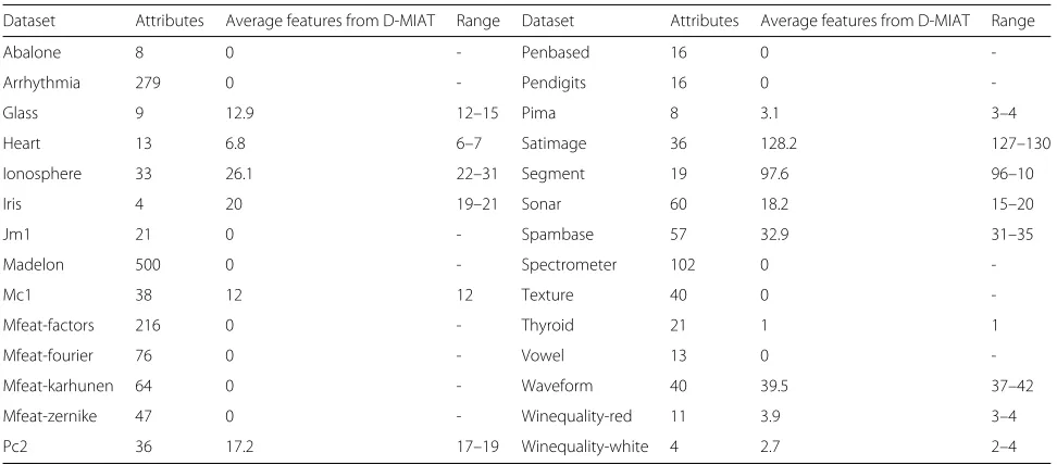
To illustrate this point, Table 2 presents the number of continuous attributes in each of the 28 datasets and the total number of attributes D-MIAT generated within each of these datasets combined with the three thresh-olds for conf we considered. As D-MIAT generated its

cuts exclusively based on 10 different iterations within the training set, it was possible that the number of features that D-MIAT generated would vary across these iterations within the 28 datasets. For example, note that the first two datasets, abalone and arrhythmia, had no features gener-ated by D-MIAT across any of the iterations and for any of the values ofconf andsupp. This shows that the D-MIAT can have a more stringent condition for generating cuts than all of the 10 canonical discretization algorithms pre-viously studied that did generate features in all of these datasets. Also note that D-MIAT generated an average of 12.9 features within the glass dataset. Based on the train-ing data, D-MIAT generated between 12 and 15 features, leading to the average being a fraction. Most times, as is the case here, the number of discretized features gener-ated by D-MIAT is less than the number of the original features. However, a notable example is found in the iris dataset which contains only four continuous attributes, but on average, D-MIAT generated 20 features. In this case, many cuts were generated for eachAjas per each one ofconf conditions in Algorithm 1.

We then checked if the features generated by D-MIAT improved predictive performance. Table 3 displays the average accuracy of the baseline data for each of the 15 files where D-MIAT generated cuts which are noted in Table 2. Please note that each of the D-MIAT supp thresholds—0 entropy in line 2, Lift of 1.5 in line 3, and lift of 2 in line 4—typically improved the prediction per-formance across all the classification algorithms. This demonstrates that the values chosen within this threshold are not extremely sensitive as all values chosen typically improve prediction accuracy. Note that all performance increases are highlighted in the table. A notable exception is the AdaBoost algorithm where no performance increase was noted (nor any decrease). Also, we note that certain algorithms, such as Naive Bayes, SVM, and logistic regres-sions consistently benefited, while the other algorithms did not. We also find that combination of the features cre-ated by the cuts from all three D-MIAT thresholds, the results of which are found in the fifth line of Table 3, yielded the best performance. As each of the cuts gener-ated by D-MIAT is significant, it is typically advantageous to add all cuts in addition to the original data. For the remainder of the paper, we will use the results of D-MIAT using all cuts as we found this yielded the highest per-formance. Thus, we overall found support for this paper’s thesis that the addition of features is not necessarily prob-lematic, unless there is a lack of added value within those attributes, even if the thresholds within the discretized cuts are not necessarily optimal.

Table 2The total number of new features generated by three D-MIAT thresholds in the each of the 28 datasets

Dataset Attributes Average features from D-MIAT Range Dataset Attributes Average features from D-MIAT Range

Abalone 8 0 - Penbased 16 0

-Arrhythmia 279 0 - Pendigits 16 0

-Glass 9 12.9 12–15 Pima 8 3.1 3–4

Heart 13 6.8 6–7 Satimage 36 128.2 127–130

Ionosphere 33 26.1 22–31 Segment 19 97.6 96–10

Iris 4 20 19–21 Sonar 60 18.2 15–20

Jm1 21 0 - Spambase 57 32.9 31–35

Madelon 500 0 - Spectrometer 102 0

-Mc1 38 12 12 Texture 40 0

-Mfeat-factors 216 0 - Thyroid 21 1 1

Mfeat-fourier 76 0 - Vowel 13 0

-Mfeat-karhunen 64 0 - Waveform 40 39.5 37–42

Mfeat-zernike 47 0 - Winequality-red 11 3.9 3–4

Pc2 36 17.2 17–19 Winequality-white 4 2.7 2–4

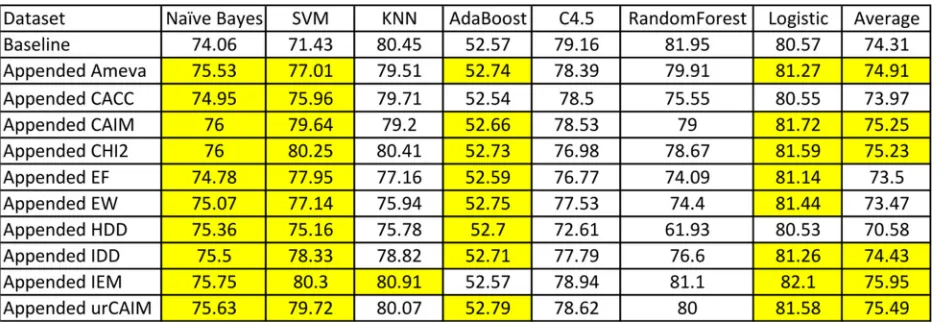
found to be correct and that using the discretized features alone would typically be useful, as has been previously been found [3,12–14]. To our surprise, we did not find this to often be the case within the 28 datasets we con-sidered. Table4, displays the average accuracy results of this experiment. The baseline here is again the average performance without discretization (A) to which we com-pared the 10 canonical discretization algorithm across the same 7 classification algorithms. Once again, each colored cell represents an improvement of a given discretization algorithm versus the baseline and note the lack of color within much of Table2. While some algorithms, particu-larly Naive Bayes and SVM, showed often large improve-ments versus the non-discretized data, the majority of classification algorithms (K-nn, AdaBoost, C4.5, Random Forest and Logistic Regression) typically did not show any improvement across the discretization algorithms in these datasets. This point is illustrated in the last column of this table, which shows that for most discretization algo-rithms, adecreasein accuracy is on average found through exclusively using discretized features. Thus, we did found that for most classification algorithms in the datasets we considered, using discretization alone was less effective than using the original features.

We found significantly more empirical support for this paper’s third research question, that using discretization in combination with the original features is more effective than using either the original set or those generated from discretization alone. The results of this experiment are found in Table5where we compare the results of the orig-inal dataset and the combination of the origorig-inal data with the features from the discretization algorithms. We again find that the Naive Bayes and SVM algorithms benefit from this combined dataset the most. When considering these two learning algorithms, improvements were now noted through combining all discretization algorithms. We note a strong improvement in the results in Table5 versus those in Table4 within the AdaBoost and Logis-tical Regression algorithms. In contrast to the results in Table 4, the average performance across all algorithms (found in the last columns of the table) now shows an improvement. Also note that almost without exception, the combined features outperformed the corresponding discretized set. For example, the average accuracy for the Ameva algorithm with C4.5 is 70.46, but this jumps to 78.39 for Ameva combined with the original data. Even when improvements were not noted, we found that performance was typically not negatively affected by the

Table 4Comparing the accuracy results from seven different classification algorithms within the original, baseline data (A) and the discretized data (D) formed from the Ameva, CACC, CAIM, Chi2, EF, EW, HDD, IDD, IEM, and ur-CAIM algorithms

addition of these features as one would assume due to the curse of dimensionality.

Despite the general support being found for the research question #3 in that using discretization to augment the original data is better than using the discretized data alone, we still note that some algorithms, particularly the K-nn, C4.5 and Random Forest learning algorithms, often did not benefit from any form of discretization. We fur-ther explore these results differences, and generally the impact of discretization on all algorithms, in Section3.4.

3.3 Using D-MIAT and other discretization algorithms as additional features

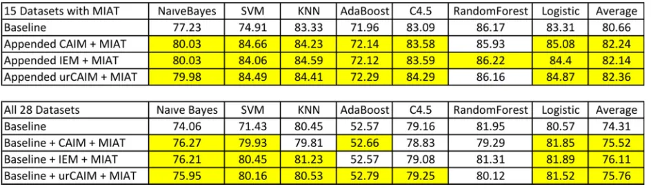
Given the finding that adding features from both D-MIAT and canonical discretization algorithms helps improve performance, we hypothesized that the combination of these features would be effective to achieve the best performance as per research question #4. To evaluate this issue, we combined the D-MIAT features with those of the best performing discretization algorithms in these

datasets– CAIM, IEM, and urCAIM. We then consid-ered the performance of this combination within the 15 datasets where D-MIAT generated some features and on average within all 28 datasets. The results of this experi-ment are found in Table6.

As can be seen from the results from the 15 datasets (top portion of Table6), the combination of discretiza-tion algorithms almost always outperforms the original data and improvements in predictive accuracy are noted in all three combinations in the Naive Bayes, SVM, K-nn, AdaBoost, C4.5, and logistic regression algorithms. The one exception seems to be the Random Forest algorithm where large performance improvements are not noted. For comparison, we also present the improvements across all 28 datasets in the bottom portion of Table 6, which include 13 datasets where there are no features generated by D-MIAT. As expected, the combination of D-MIAT was somewhat less significant once again demonstrating the benefit of adding the features from D-MIAT. Overall, and on average across the algorithms we considered, we

Table 6Combining D-MIAT with discretization features yields the highest performance when considering the 15 datasets where D-MIAT added features, and on average across all 28 datasets

found that this combination was the most successful, with prediction accuracies typically improving by over 1%. Thus, we found the thesis #4 to typically be correct and using D-MIAT in conjunction with existing discretization algorithms is recommended to enrich the set of features to be considered.

3.4 Discussion and future work

We were somewhat surprised that using discretization alone was not as successful as it has been previously found with such classification algorithms as Random Forests and C4.5 [3,12–14]. We believe that differences in the datasets being analyzed is likely responsible for these gaps. As such, we believe that an important open question is to predict when discretization will be successful, given the machine learning algorithm and the dataset used for input. In con-trast, we found that D-MIAT yielded more stable results as it typically only improved the performance, something other discretization algorithms did not do, especially for these two learning algorithms. We are now exploring how to make other discretization algorithms similarly more stable.

We note that the pipeline described in this paper of using D-MIAT and discretized features in addition to the original data was most effective with algorithms without discretization, namely the Naive Bayes, SVM, and Logis-tic Regression classification algorithms. Conversely, this approach was less effective with methods having a dis-cretization component, particularly with C4.5, Random Forests, and AdaBoost algorithms. It has been previously noted that C4.5 has a localized discretization component (re–applied at each internal node of the decision tree) and thus may gain less from adding globally discretized fea-tures, which are split into the same intervals across all decision tree nodes Dougherty et al. [3]. Similarly, the decision stumps used as weak classifiers in AdaBoost per-form essentially a global discretization and thus may have made it less likely to benefit from the globally discretized features added by D-MIAT, something that is evident from

Table3. As can be noted from Table6, the Random Forest algorithm benefited the least from the pipeline described in this paper– again possibly due to its discretization component. We hope to further study when and why algorithms with an inherent discretization component still benefit from additional discretization. Additionally, it seems that the K-nn algorithm, despite not having a dis-cretization component, benefits less from the proposed pipeline than other algorithms. It seems plausible this is because this algorithm is known to be particularly sen-sitive to the curse of dimensionality [24, 25] and thus this specific algorithm does not benefit from the pro-posed approach while other classification algorithms are less sensitive to it. We plan to study this complex issue in our future research.

thresholds used in this study represent an optimal value, or set of values, for all datasets. One potential solution to this would be to develop a metacognition mechanism for learning these thresholds for a given dataset. Similarly, it is possible that a form of metacognition could be added to machine learning algorithms as has been generally sug-gested within neural networks [27] to help achieve this goal.

4 Conclusions

In this paper, we present a paradigm shift in how dis-cretization can be used. To date, disdis-cretization has typi-cally been used as a pre-processing step which removes the original attribute values, replacing them with dis-cretized intervals. Instead, we suggest using the features that are generated by discretization to extend the dataset by using both the discretized and non-discretized versions of the data. We have demonstrated that discretization can often be used to generate new features which should be used in addition to the dataset’s non-discretized features. The D-MIAT algorithm we present in this paper is based on this assumption. This is because D-MIAT will only dis-cretize values with particularly strong indications based on high confidence, yet relatively low support for the tar-get class, as it assumes that classification algorithms will also be using the original data. We also show that other canonical discretization algorithms can be used in a simi-lar fashion, and in fact a combination of the original data with D-MIAT and discretized features from other algo-rithms yields the best performance. We are hopeful that the ideas presented in this paper will advance the use of discretization and its application to new datasets and algorithms.

Endnotes

1_{http://www.uco.es/grupos/kdis/wiki/ur-CAIM/}

2_{The file “run_all.m” found in this zip was used to run}

D-MIAT in batch across all files in a specified directory.

Funding

The work by Avi Rosenfeld, Ron Illuz, and Dovid Gottesman was partially funded by the Charles Wolfson Charitable Trust.

Authors’ contributions

AR, RI, and DG were responsible for data collection and analysis. AR and ML were responsible for the algorithm development and writing of the paper. All authors read and approved the final manuscript.

Competing interests

The authors declare that they have no competing interests.

Publisher’s Note

Springer Nature remains neutral with regard to jurisdictional claims in published maps and institutional affiliations.

Author details

1_{Jerusalem College of Technology, Jerusalem, Israel.}2_{Ben Gurion University of} the Negev, Beersheba, Israel.

Received: 23 May 2017 Accepted: 4 January 2018

References

1. S Garcia, J Luengo, JA Sáez, V Lopez, F Herrera, A survey of discretization techniques: Taxonomy and empirical analysis in supervised learning. IEEE Trans. Knowl. Data Eng.25(4), 734–750 (2013)

2. MR Chmielewski, JW Grzymala-Busse, Global discretization of continuous attributes as preprocessing for machine learning. Int. J. Approx. Reason.

15(4), 319–331 (1996)

3. J Dougherty, R Kohavi, M Sahami, et al, inMachine learning: proceedings of the twelfth international conference,volume 12. Supervised and unsupervised discretization of continuous features (Morgan Kaufmann Publishers, San Francisco, 1995), pp. 194–202

4. H Liu, R Setiono, Feature selection via discretization. IEEE Trans. Knowl. Data Eng.9(4), 642–645 (1997)

5. LA Kurgan, KJ Cios, Caim discretization algorithm. IEEE Trans. Knowl. Data Eng.16(2), 145–153 (2004)

6. L Gonzalez-Abril, FJ Cuberos, F Velasco, JA Ortega, Ameva: An

autonomous discretization algorithm. Expert Syst. Appl.36(3), 5327–5332 (2009)

7. FEH Tay, L Shen, A modified chi2 algorithm for discretization. IEEE Trans. Knowl. Data Eng.14(3), 666–670 (2002)

8. P Yang, J-S Li, Y-X Huang, Hdd: a hypercube division-based algorithm for discretisation. Int. J. Syst. Sci.42(4), 557–566 (2011)

9. C-J Tsai, C-I Lee, W-P Yang, A discretization algorithm based on class-attribute contingency coefficient. Inf. Sci.178(3), 714–731 (2008) 10. FJ Ruiz, C Angulo, N Agell, Idd: a supervised interval distance-based

method for discretization. IEEE Trans. Knowl. Data Eng.20(9), 1230–1238 (2008)

11. A Cano, DT Nguyen, S Ventura, KJ Cios, ur-caim: improved caim discretization for unbalanced and balanced data. Soft Comput.20(1), 173–188 (2016)

12. JL Lustgarten, V Gopalakrishnan, H Grover, S Visweswaran, inAMIA. Improving classification performance with discretization on biomedical datasets (American Medical Informatics Association (AMIA), Bethesda, 2008)

13. JL Lustgarten, S Visweswaran, V Gopalakrishnan, GF Cooper, Application of an efficient bayesian discretization method to biomedical data. BMC Bioinformatics.12(1), 309 (2011)

14. DM Maslove, T Podchiyska, HJ Lowe, Discretization of continuous features in clinical datasets. J. Am. Med. Inform. Assoc.20(3), 544–553 (2013) 15. A Rosenfeld, DG Graham, R Hamoudi, R Butawan, V Eneh, S Khan, H Miah,

M Niranjan, LB Lovat, in2015 IEEE International Conference on Data Science and Advanced Analytics, DSAA. MIAT: A novel attribute selection approach to better predict upper gastrointestinal cancer (Campus des Cordeliers, Paris, 2015), pp. 1–7

16. I Guyon, A Elisseeff, An introduction to variable and feature selection. J. Mach. Learn. Res.3(Mar), 1157–1182 (2003)

17. I Guyon, An introduction to variable and feature selection. J. Mach. Learn. Res.3, 1157–1182 (2003)

18. Y Saeys, I Inza, P Larrañaga, A review of feature selection techniques in bioinformatics. Bioinformatics.23(19), 2507–2517 (2007)

19. RA Hamoudi, A Appert, et al, Differential expression of nf-kappab target genes in malt lymphoma with and without chromosome translocation: insights into molecular mechanism. Leukemia.24(8), 1487–1497 (2010)

20. Z Zheng, R Kohavi, L Mason, inProceedings of the seventh ACM SIGKDD international conference on Knowledge discovery and data mining. Real world performance of association rule algorithms (ACM, New York, 2001), pp. 401–406

21. J Alcalá-Fdez, A Fernández, J Luengo, J Derrac, S García, L Sanchez, F Herrera, Keel data-mining software tool: data set repository, integration of algorithms and experimental analysis framework. J. Mult. Valued Log. Soft. Comput.17, 255–287 (2011)

22. M Lichman,UCI Machine Learning Repository. (University of California, School of Information and Computer Science, Irvine, 2013).http://archive. ics.uci.edu/ml

24. JsH Friedman, et al.,Flexible metric nearest neighbor classification.Technical report, Technical report. (Department of Statistics, Stanford University, 1994)

25. DW Aha, Editorial. Artif. Intell. Rev.11, 7–10 (1997)

26. C Watkins,Learning about learning enhances performance(Institute of Education, University of London, 2001)

27. R Savitha, S Suresh, N Sundararajan, Metacognitive learning in a fully complex-valued radial basis function neural network. Neural Comput.