Vibrato in Singing Voice: The Link between
Source-Filter and Sinusoidal Models
Ixone Arroabarren
Departamento de Ingenier´ıa El´ectrica y Electr´onica, Universidad P´ublica de Navarra, Campus de Arrosadia, 31006 Pamplona, Spain Email:[email protected]
Alfonso Carlosena
Departamento de Ingenier´ıa El´ectrica y Electr´onica, Universidad P´ublica de Navarra, Campus de Arrosadia, 31006 Pamplona, Spain Email:[email protected]
Received 4 July 2003; Revised 30 October 2003
The application of inverse filtering techniques for high-quality singing voice analysis/synthesis is discussed. In the context of source-filter models, inverse filtering provides a noninvasive method to extract the voice source, and thus to study voice quality. Although this approach is widely used in speech synthesis, this is not the case in singing voice. Several studies have proved that inverse filtering techniques fail in the case of singing voice, the reasons being unclear. In order to shed light on this problem, we will consider here an additional feature of singing voice, not present in speech: thevibrato. Vibrato has been traditionally studied by sinusoidal modeling. As an alternative, we will introduce here a novel noninteractive source filter model that incorporates the mechanisms of vibrato generation. This model will also allow the comparison of the results produced by inverse filtering techniques and by sinusoidal modeling, as they apply to singing voice and not to speech. In this way, the limitations of these conventional techniques, described in previous literature, will be explained. Both synthetic signals and singer recordings are used to validate and compare the techniques presented in the paper.
Keywords and phrases:voice quality, source-filter model, inverse filtering, singing voice, vibrato, sinusoidal model.
1. INTRODUCTION
Inverse filtering provides a noninvasive method to study voice quality. In this context, high-quality speech synthesis is developed using a source-filter model, where voice texture is controlled by glottal source characteristics. Efforts to ap-ply this approach to singing voice have failed, the reasons being not clear: either the unsuitability of the model, or the different range of frequencies, or both, could be the cause. The lyric singers, being professionals, have an efficiency re-quirement, and as a result, they are educated to change their formants position moving them towards the first harmonics position, what could also be another reason of the model’s failure [1].
This paper purports to shed light on this problem by comparing two salient methods for glottal source and vo-cal tract response (VTR) estimation, with a novel frequency-domain method proposed by the authors. In this way, the inverse filtering approach will be tested in singing voice anal-ysis. In order to have a benchmark, the source-filter model will be compared to sinusoidal model and this comparison will be performed thanks to the particular feature of singing voice: vibrato.
Regarding the voice production models, we can distin-guish two approaches as follows.
(ii) On the other hand, Non Interactive Models separate the glottal source and the VTR, and both are independently modeled as linear time-varying systems. This is the case of the source-filter model proposed by Fant in [6]. The VTR is modeled as an all-pole filter, in the case of nonnasal sounds. For the glottal source several waveform models have been proposed [7,8,9], but all of them try to include some of the features of the source-tract interaction, typically the asym-metric shape of the pulse. These models provide a high qual-ity synthesis framework for the speech with a low compu-tational complexity. The synthesis is preceded by an anal-ysis stage, which is divided into two steps: an inverse fil-tering step where the glottal source and the VTR are sepa-rated [9,10,11,12,13] and a parameterization step where the most relevant parameters of both elements are obtained [14,15,16].
In general, inverse filtering techniques yield worse re-sults as the fundamental frequency increases, as is the case of women and children in speech and singing voice. In the latter case, singing voice, the number of published works is very scarce [1,17]. In [1], the glottal source features are stud-ied in speech and singing voice by acoustic and electroglotto-graphic signals [18,19]. From these works, it is not apparent which is the main limitation of inverse filtering in singing voice. It might be possible that the source-tract interaction was more complex than in speech, what would represent a paradox in the noninteractive assumption [20]. Other rea-son mentioned in [1] is that perhaps the glottal source mod-els used in speech are not suitable for singing voice. These statements are not demonstrated, but are interesting ques-tions that should be answered.
On the other hand, in [17] the noninteractive source-filter model is used as a high-quality singing voice synthesis approach. The main contribution of that work is the devel-opment of an analysis procedure that estimates the param-eters of the synthesis model [12,21]. However, there is no evidence that could point to differences between speech and singing as it is indicated in [1].
One of the goals of the present work is to clarify whether the noninteractive models are able to model singing voice in the same way as high-quality speech, or on the contrary, the source-tract interaction is different from speech, and pre-cludes this linear model assumption. If the noninteractive model could model singing voice, the reason of the failure of inverse filtering techniques would be just the high funda-mental frequency of singing voice.
To this end, we will compare in this paper three diff er-ent inverse filtering techniques, one of them novel and pro-posed recently by the authors in order to obtain the source-filter decomposition. Though they work correctly for speech and low-frequency signals, we will show their limitations as the fundamental frequency increases. This is described in
Section 2.
Since fundamental frequency in singing voice is higher than in speech, it seems obvious that the above-mentioned methods fail, apparently due to the limited spectral informa-tion provided in high pitched signals. To compensate for that, we claim that the introduction of a feature such as vibrato
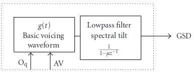
Singing voice Lip radiation
diagram 1−l·z−1 VTR
Glottal source
Figure1: Noninteractive source-filter model of voice production system.
may serve to increase the information available by virtue of the frequency modulated nature, and therefore wider band-width, of vibrato [22,23,24]. Frequency variations are in-fluenced by the VTR, and this effect can be used to obtain information about it.
With this in mind, it is not surprising that vibrato has been traditionally analyzed by sinusoidal modeling [25,26], the most important limitation being the impossibility to sep-arate the sound generation and the VTR. In Section 3, we will take a step forward by introducing a source-filter model, which accounts for the physical origin of the main features of singing voice. Making use of this model, we will also demon-strate how the simpler sinusoidal model can serve to obtain a complementary information to inverse filtering, particularly in those conditions where the latter method fails.
2. INVERSE FILTERING
Along this section, the noninteractive source-filter model, depicted inFigure 1, will be considered and some of the pos-sible estimation algorithms for it will be reviewed.
According to the block diagram inFigure 1, singing voice production can be modeled by a glottal source excitation that is linearly modified by the VTR and the lip radiation dia-gram. Typically, the VTR is modeled by an all-pole filter, and relying on the linearity of the model, the lip radiation sys-tem is combined with the glottal source, in such a way that the glottal source derivative (GSD) is considered as the vocal tract excitation.
In this context, during the last decades many inverse fil-tering algorithms to estimate the model elements have been proposed. This technique is usually accomplished in two steps. In the first one, the GSD waveform and the VTR are estimated. In the second one, these signals are parameterized in a few numerical values. This whole analysis can be practi-cally implemented in several ways. For the sake of clarity, we can group these possibilities into two types.
Voice source parameters Voice source
parameters optimization Preemphasis
Voice source model
Covariance LPC
Vocal tract parameters Preemphasis
Speech
Figure2: Block diagram of the AbS inverse filtering algorithm.
(ii) The procedures in the second group split the whole process into two stages. Regarding the first step, different inverse filtering techniques are proposed, [11,13]. These al-gorithms remove the GSD effect from the speech signal and the VTR is obtained by linear prediction (LP) [28] or alterna-tively by discrete all-pole (DAP) modeling [29], which avoids the fundamental frequency dependence of the former.
For this comparative study three inverse filtering ap-proaches have been selected. The first one is theanalysis by synthesis(AbS) procedure presented in [9], the second one is the one proposed by the authors in [13],Glottal Spectrum Based(GSB) inverse filtering. In this way, both groups of al-gorithms mentioned above are represented. In addition, the Closed Phase Covariance(CPC) [10] has been added to the comparison. This approach is difficult to classify because it only obtains the VTR, as it is the case in the second group, but it is a time domain implementation as in the first one. The most interesting feature of this algorithm is that it is less affected by the formant ripple due to the source-tract inter-action, because it only takes into account the time interval when the vocal folds are closed. In what follows, the three approaches will be shortly described, and finally compared.
2.1. Analysis by synthesis
This inverse filtering algorithm was proposed in [9]. It is based on covariance LPC [29], but the least squares error is modified in order to include the input of the system:
E=
N−1
n=0
s(n)−sˆ(n)2
=
N−1
n=0
s(n)−
p
k=1
aks(n−k) +ap+1g(n) 2
, (1)
whereg(n) represents the GSD, and
H(z)= ap+1 1−kp=1akz−k
(2)
represents the VTR. Since neither VTR nor GSD parameters are known, an iterative algorithm is proposed and a
simul-taneous search is developed. The block diagram of the algo-rithm is represented inFigure 2.
As in covariance LP without source, this approach al-lows shorter analysis windows. However, the stability of the system is not guaranteed and a stabilization step must be in-cluded with this purpose. Also, and since it is a time domain implementation, the voice source model must be synchro-nized with the speech signal and a high sampling frequency is mandatory in order to obtain satisfactory results. As a result, the computational load is also high. Regarding the GSD pa-rameter optimization, it is dependent on the chosen model. In the results shown inSection 2.4, the LF model is selected because it is one of the most powerful GSD models, and it allows an independent control of the three main features of the glottal source: open quotient, asymmetry coefficient and spectral tilt. The disadvantage of this model is its computa-tional load. For more details on the topic readers are referred to [8].
Regarding fundamental frequency limits, it is shown in [1] that this algorithm provides unsatisfactory results for medium and high pitched signals.
2.2. Glottal spectrum based inverse filtering
This technique was proposed by the authors in [13] and will be briefly described here. Unlike the technique described in the previous section, it is essentially a frequency domain im-plementation. In the AbS approach, the GSD effect was in-cluded in the LP error, and the AR coefficients were obtained by Covariance LPC. In our case, a short term spectrum of speech is considered (3 or 4 fundamental periods), and the GSD effect is removed from the speech spectrum. Then, the AR coefficients of (2) are obtained by the DAP modeling [29].
For this spectral implementation, the KLGLOTT88 model [7] has been considered. It is less powerful than the LF model, but of a simpler implementation.
GSD
Figure3: Block diagram of the KLGLOTT88 model.
Vocal tract
Figure4: Block diagram of the GSB inverse filtering algorithm.
In our inverse filtering algorithm, once the short term spectrum is calculated, the glottal source effect is removed, by spectral division, by using the spectrum of the basic voicing waveform (3), which can be directly obtained by the Fourier transform of the basic voicing waveform [30]:
G(f)= 27 AV
The spectral tilt (ST) and the VTR are combined in an (N+ 1)th order all-pole filter. The block diagram of the algorithm is shown inFigure 4.
Since DAP modeling is the most important part of the algorithm, we should explain its rationale. In classical auto-correlation LP [28], it is a well-known effect that as funda-mental frequency increases the resulting transfer function is biased by the spectral peaks of the signal. This happens be-cause the signal is assumed to be the impulse response of the system, and this assumption is obviously not entirely correct. In order to avoid this problem, an alternative proposed in [29] is to obtain the LP error based on the spectral peaks, instead of on the time domain samples. Unfortunately, this error calculation is based on an aliased version of the right autocorrelation of the signal, and this aliasing grows as the fundamental frequency increases. Then, the resulting trans-fer function is not correct again. To solve this problem, the DAP modeling uses the Itakura-Saito error, instead of the least squares error, and it can be shown that the error is min-imized using only the spectral peaks information. The de-tails of the algorithm are explained in [29]. This technique allows higher fundamental frequencies than classical auto-correlation LP, but for proper operation requires an enough number of spectral peaks in order to estimate the right
trans-GSD
Figure5: Closed phase interval in voice.
Closed
Figure6: Closed phase covariance (CPC).
fer function. So, this inverse filtering algorithm will also have a limit in the highest achievable fundamental frequency.
2.3. Closed phase covariance
This inverse filtering technique was proposed in [31]. It is also based on covariance LP, as the AbS approach explained above. However, instead of removing the effect of the GSD from a long speech interval, the classical covariance LP takes only into account a portion of a single cycle where the vocal folds are closed. In this way, and in the considered time in-terval, there is no GSD information to be removed, and the application of covariance LP will lead to the right transfer function. Considering the linearity of the model shown in
Figure 1, the closed phased interval will be the time interval
where the GSD is zero. This situation is depicted inFigure 5. The most difficult step in this technique is to detect the closed phase in the speech signal. In [10], a two-channel speech processing is proposed, making use of electroglotto-graphic signals to detect the closed phase. Electroglottogra-phy (EGG) is a technique used to indirectly register laryngeal behavior by measuring the electrical impedance across the throat during speech. Rapid variation in the conductance is mainly caused by movement of the vocal folds. As they ap-proximate and the physical contact between them increases, the impedance decreases, what results in a relatively higher current flow through the larynx structures. Therefore, this signal will provide information about the contact surface of the vocal cords.
The complete inverse filtering algorithm is represented in
GSB CPC AbS Original GSD
0.02 0.025 0.03 0.035 0.04 0.045 0.05 0.055 0.06 Time (s)
(a)
GSB CPC AbS Original GSD
0.014 0.016 0.018 0.02 0.022 0.024 0.026 Time (s)
(b)
GSB CPC AbS Original VTR
0 1000 2000 3000 4000 5000 6000 7000 Frequency (Hz)
−50 −40 −30 −20 −10 0 10 20 30 40 50
A
m
plitude
(dB)
(c)
GSB CPC AbS Original VTR
0 1000 2000 3000 4000 5000 6000 7000 Frequency (Hz)
−40 −30 −20 −10 0 10 20 30 40 50
A
m
plitude
(dB)
(d)
Figure7: (a) Estimated GSD.F0=100 Hz, vowel “a.” (b) Estimated GSD.F0=300 Hz, vowel “a.” (c) Estimated VTR.F0=100 Hz, vowel “a.” (d) Estimated VTR.F0=300 Hz, vowel “a.”
InFigure 6, a GCI detection block [27] is included,
be-cause, even though both acoustic and electroglottographic signals are simultaneously recorded, there is a propaga-tion delay between the acoustic signal recorded on the microphone and the impedance variation at the neck of the singer. Thus, a precise synchronization is mandatory.
Since this technique is based on the covariance LP, it may work with very short window lengths. However, as the fun-damental frequency increases, the time length of the closed phase gets shorter, and there is much less information left for the vocal tract estimation. This fact imposes a fundamental frequency limit, even using the covariance LP.
2.4. Practical results
Once the basics of three inverse filtering techniques have been presented and described, they will be compared by sim-ulations and also by making use of natural singing voice records. The main goal of this analysis is to see how the three techniques are compared in terms of their fundamental fre-quency limitations.
2.4.1. Simulation results
First, the non interactive model for voice production shown
in Figure 1will be used in order to synthesize some
artifi-cial signals for test. The lip radiation effect and the glottal source are combined in a mathematical model for the GSD, also making use of the LF model. It is well known [1,17] that the formant position can affect inverse filtering results. In [3], it is also shown that the lower first formant central fre-quency is, the higher is the source-tract interaction. So, the interaction is higher in vowels where the first format central frequency is lower. Therefore, and in order to cover all pos-sible situations, two vocal all-pole filters have been used for synthesizing the test signal: one representing Spanish vowel “a,” and the other one representing Spanish vowel “e.” In this latter case, the first formant is located at lower frequencies.
GSB
Figure8: Fundamental frequency dependence. (a) ErrorF1in vowel “a.” (b) ErrorF1in vowel “e.” (c) ErrorGSDin vowel “a.” (d) ErrorGSDin vowel “e.”
7d, the glottal GSD and the VTR estimated by the three ap-proaches are shown for two different fundamental frequen-cies. Note that in them, and in other figures, DC level has been arbitrarily modified to facilitate comparisons.
Comparing the results obtained by the three inverse fil-tering approaches, it is shown that as fundamental frequency increases the error in both GSD and VTR increases. Recall-ing the implementation of the algorithms, the CPC uses only the time interval where the GSD is zero. When the funda-mental frequency is low, it is possible to see that the result of this technique is the closest one to the original one. In the case of the other two techniques, both have slight vari-ations in the closed phase, because in both cases the glottal source effect is removed from the speech signal in an approx-imated manner. Otherwise, when the fundamental frequency is high, the AbS approach leads comparatively to the best re-sult. However, it provides neither the right GSD, nor the right VTR.
InFigure 8, the relative error in the first formant central
frequency and the error in the GSD are represented for the
three methods, calculated according to the following expres-sions:
whereF1represents the first formant central frequency and
g(n) and ˆg(n) are the original and estimated GSD waveforms, respectively.
GSB CPC AbS
1.269 1.274 1.279 1.284 1.289 1.294 1.299 Time (s)
(a)
GSB CPC AbS
0 1000 2000 3000 4000 5000 6000 7000 Frequency (Hz)
−100 −80 −60 −40 −20 0
A
m
plitude
(dB)
(b)
GSB CPC AbS
0.765 0.767 0.769 0.771 0.773 0.775 0.777 Time (s)
(c)
GSB CPC AbS
0 1000 2000 3000 4000 5000 6000 7000 Frequency (Hz)
−100 −80 −60 −40 −20 0
A
m
plitude
(dB)
(d)
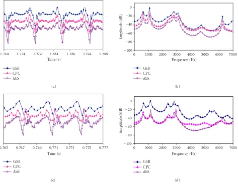
Figure9: (a) Estimated GSD.F0=123 Hz, vowel “a.” (b) Estimated VTR.F0=123 Hz, vowel “a.” (c) Estimated GSD.F0=295 Hz, vowel “a.” (d) Estimated VTR.F0=295 Hz, vowel “a.”
2.4.2. Natural singing voice results
For this analysis, three male professional singers were recorded: two tenors and one baritone. They were asked to sing notes of different fundamental frequency values, in or-der to register samples of all of their tessitura. Besides, diff er-ent vocal tract configurations are considered, and thus, this exercise was repeated for the five Spanish vowels “a,” “e,” “i,” “o,” “u.” The singing material was recorded in a professional studio, in such a way that reverberation was reduced as much as possible. Acoustic and electroglottographic signals were synchronously recorded, with a bandwidth of 20 KHz, and stored in.wav format. In order to remove low frequency am-bient noise, the signals were filtered out by a high pass lin-ear phase FIR filter whose cut-offfrequency was set to a 75% of the fundamental frequency. In the case of electroglotto-graphic signals, this filtering was also applied because of low frequency artifacts typical of this kind of signals due to larynx movements.
In Figures 9a to 9c, the results obtained for different fundamental frequencies and vowel “a,” for the same singer,
are shown. These results are also representative of the other singers’ recordings and of the different vowels.
By comparing Figures9aand9c, it is possible to conclude that in the case of a low fundamental frequency, the three al-gorithms provide very close results. In the case of CPC, the GSD presents less formant ripple in the closed phase interval. Regarding the VTR, the central frequencies of the formants and the frequency responses are very similar. Nevertheless, in the case of a high fundamental frequency, the resulting GSD of the three analyses are very different from those of
Figure 9a, and also from the waveform model provided by
the LF model. Also, the calculated VTR is very different for the three methods. Thus, conclusions with natural recorded voices are similar to those obtained with synthetic signals.
3. VIBRATO IN SINGING VOICE
3.1. Definition
In Section 2, inverse filtering techniques, successfully
processing. It has been shown that as fundamental frequency increases, they reach a limit and thus an alternative technique should be used. As we will show in this section, the introduc-tion of vibrato in singing voice provides more informaintroduc-tion about what can be happening.
Vibrato in singing voice could be defined as a small quasiperiodic variation of the fundamental frequency of the note. As a result of this variation, all of the harmonics of the voice will also present an amplitude variation, because of the filtering effect of the VTR. Due to these nonstationary char-acteristics of the signal, singing voice has been modeled by the modified sinusoidal model [25,26]:
s(t)=
N−1
i=0
ai(t) cosθi(t) +r(t), (5)
where
θi(t)=2π t
−∞ fi(τ)dτ (6)
andai(t) is theinstantaneous amplitude of the partial,fi(t) the instantaneous frequency of the partial, andr(t) thestochastic residual.
The acoustic signal is composed by a set of components, (partials), whose amplitude and frequency change with time, plus a stochastic residual, which is modeled by a spectral density time-varying function. Also in [25,26], detailed in-formation is given on how these time-varying characteristics can be measured.
Of the two features of a vibrato signal, frequency and amplitude variations, frequency is the most widely stud-ied and characterized. In [32, 33], the instantaneous fre-quency is characterized and decomposed into three main components which account for three musically meaningful characteristics, respectively. Namely,
f(t)=i(t) +e(t) cosϕ(t), (7)
where
ϕ(t)=2π t
−∞r(τ)dτ (8)
f(t) being the instantaneous frequency,i(t) theintonationof the note, which corresponds to slow variations of pitch;e(t) represents theextent or amplitude of pitch variations, and
r(t) represents therateor frequency of pitch variations. All of them are time-dependent magnitudes and rely on the musical context and singer’s talent and training. In the case of intonation, its value depends on the sung note, and thus, on the context. But extent and rate are mostly singer-dependent features, typical values being a 10% of the intona-tion value and 5 Hz, respectively.
Regarding the amplitude variation of the harmonics dur-ing vibrato, a well-established parameterization is not ac-cepted, and probably it does not exist, because this varia-tion is different for all of the harmonics. It is therefore not strange that amplitude variation has been the topic of
inter-0 500 1000 1500 2000 2500 3000 3500 4000 4500 5000 Frequency (Hz)
−90 −80 −70 −60 −50 −40 −30 −20 −10 0
A
m
plitude
(dB)
Figure10: AM-FM representation for the first 20 harmonics. Ane-choic tenor recordingF0=220 Hz, vowel “a.”
est of some few papers. The first work on this topic is [34], where the perceptual relevance on spectral envelope discrim-ination of the instantaneous amplitude is proven. In [22], the relevance of this feature is experimentally demonstrated in the case of synthesis of singing voice. Also, its physical cause is tackled and a representation in terms of the instantaneous amplitude versus instantaneous frequency of the harmonics is introduced for the first time. This representation is pro-posed as a means of obtaining a local information of the VTR in limited frequency ranges. Something similar is done in [35], where the singing voice is synthesized using this lo-cal information of the VTR. We have also contributed in this direction, for instance in [23], where the instantaneous am-plitude is decomposed in two parts. The first one represents the sound intensity variation and the other one represents the amplitude variation determined by the local VTR, in an attempt to split the contribution of the source and the vocal tract. Moreover, in [24], different time-frequency processing tools have been used and compared in order to identify the relationship between instantaneous amplitude and instanta-neous frequency.
In that work, the AM-FM representation is defined as the instantaneous amplitude versus instantaneous frequency representation, with time being an implicit parameter. This representation is compared to the magnitude response of an all-pole filter, which is typically used for VTR modeling. Two main conclusions are derived, the first one is that only when anechoic recordings are considered, these two representa-tions can be compared. Otherwise, the instantaneous mag-nitudes will be affected by reverberation. The second one is that, as a frequency modulated input is considered, and fre-quency modulation is not a linear operation, the phase of the all-pole system will affect the AM-FM representation, leading to a different representation than the vocal tract magnitude response. However the relevance of this effect depends on the formant bandwidth and vibrato characteristics, vibrato rate in this case. It was also shown that in natural vibrato the phase effect of VTR is not noticeable, because vibrato rate is slow comparing to formant bandwidths.
Figure 10 constitutes a good example of the kind of
harmonic’s instantaneous amplitude is represented versus its instantaneous frequency. For this case, only two vibrato cy-cles, where the vocal intensity does not change significantly, have been considered. As the number of harmonic increases, the frequency range swept by each harmonic widens. Com-paringFigure 10andFigure 9b, the AM-FM representation of the former one is very similar to the VTR of Figure 9b. However, in the case of the AM-FM representation, no source-filter separation has been made, and thus both ele-ments are melted in that representation. The results obtained by other authors [22,35] are quite similar regarding the in-stantaneous amplitude versus inin-stantaneous frequency rep-resentation, however, in those works no comment is made about the conditions of recordings.
3.2. Simplified noninteractive source-tract model with vibrato
The main conclusion from the results presented above could be that vibrato might be used in order to extract more in-formation about glottal source and VTR in singing voice. Therefore, we will propose here a simplified noninteractive source-filter model with vibrato that will be a signal model of vibrato production and will explain the results provided by sinusoidal modeling. We will first make some basic as-sumptions regarding what is happening with GSD and VTR during vibrato. These assumptions are based on perceptual aspects of vibrato, and on the AM-FM representation for nat-ural singing voice.
(1) The GSD characteristics remain constant during vi-brato, and only the fundamental frequency of the voice changes. This assumption is justified by the fact that perceptually there is no phonation change during a single note.
(2) The intensity of the sound is constant, at least during one or two vibrato cycles.
(3) The VTR remains invariant during vibrato. This as-sumption relies on the fact that vocalization does not change along the note.
(4) The three vibrato characteristics remain constant. This assumption is not strictly true, but their time constants are considerably larger than the signal fundamental period.
Taking into account these four assumptions, the simpli-fied noninteractive source-filter model with vibrato could be represented by the block diagram inFigure 11.
Based on this model, we will simulate the produc-tion of vibrato. The GSD characteristics are the same as
in Section 2.4, and the VTR has been implemented as an
all-pole filter whose frequency response represents Spanish vowel “a.” A frequency variation, typical of vibrato, has been applied to the GSD with a 120 Hz intonation, an extent of 10% of the intonation value, and a rate of 5,5 Hz. All of them are kept constant in the complete register.
We have applied to the resulting signal both inverse fil-tering (where the presence or absence of vibrato does not fluence the algorithm), and sinusoidal modeling, where
in-Singing voice VTR
H(z)= 1 1−pk=1akz−k
F0(t): vibrato intonation rate extent Glotal source
derivative LF model
Oq
ft
α
Figure11: Noninteractive source-filter model with vibrato.
stantaneous amplitude and instantaneous frequency of each harmonic need to be measured. Results obtained for this sim-ulation are shown in Figures12,13,14, and15. InFigure 12a
inverse filtering results are shown for a short window analy-sis. When fundamental frequency is low, GSD and VTR are well separated. In Figures12a,13a, sinusoidal modeling re-sults are shown. The frequency variations of the harmonics of the signal are clearly observed and, as a result, the am-plitude variation. On the other hand, inFigure 14, the AM-FM representation of the partials is shown. Taking into ac-count the AM-FM representation of every partial, and com-paring this to the VTR shown in Figure 12a, it is possible to conclude that a local information of the VTR is provided by this method. However, as no source-filter decomposition has been developed, each AM-FM representation is shifted in amplitude depending on the GSD spectral features. This effect is a result of keeping GSD parameters constant during vibrato. Comparing Figures14and15, it can be noticed that if the GSD magnitude spectrum is removed from the AM-FM representation of the harmonics, the resulting AM-FM rep-resentation would provide only VTR information. The result of this operation is shown inFigure 16.
For this simplified noninteractive source-filter model with vibrato, instantaneous parameters of sinusoidal model-ing provide a complementary information about both GSD and VTR. When inverse filtering works, the GSD effect can be removed from the AM-FM representation provided by si-nusoidal modeling and only the information of the VTR re-mains.
3.3. Natural singing voice
The relationship between these two signal models, noninter-active source-filter model and sinusoidal model, has been es-tablished for a synthetic signal where vibrato has been in-cluded under the four assumptions stated at the beginning of the section. Now, the question is whether this relationship holds in natural singing voice too. Therefore, both kinds of signal analysis will be now applied to natural singing voice. In order to get close to simulation conditions, some precautions have been taken in the recording process.
Original GSD Inverse filtered GSD
0.402 0.407 0.412 0.417 0.422 0.427 0.432 Time (s)
(a)
Original VTR Inverse filtered VTR
0 2000 4000 6000
Frequency (Hz) −50
−40 −30 −20 −10 0 10 20 30
A
m
plitude
(dB)
(b) Figure12: Inverse filtering results. GSB inverse filtering algorithm. (a) GSD. (b) VTR.
0 0.2 0.4 0.6 0.8
Time (s) 0
500 1000 1500 2000 2500
Fre
q
u
en
cy
(H
z)
(a)
0 0.2 0.4 0.6 0.8
Time (s) 35
40 45 50 55 60 65 70 75 80
A
m
plitude
(dB)
(b)
Figure13: Sinusoidal modeling results. (a) Instantaneous frequency. (b) Instantaneous amplitude.
0 500 1000 1500 2000 2500 3000
Frequency (Hz) 0
10 20 30 40 50 60 70 80
A
m
plitude
(dB)
Figure14: AM-FM representation.
(2) Recordings have been done in a studio where reverber-ations are reduced but not completely eliminated as in an anechoic room. In this situation, the AM-FM rep-resentation will present slight variations from the ac-tual VTR, but it is still possible to develop a qualitative study.
Short term spectrum Spectral peaks
0 500 1000 1500 2000 2500 3000
Frequency (Hz) −70
−60 −50 −40 −30 −20 −10 0
A
m
plitude
(dB)
Figure15: GSD short term spectrum. Blackman-Harris window.
AM-FM representation without source VTR
0 500 1000 1500 2000 2500 3000
Frequency (Hz) 40
50 60 70 80 90 100 110
A
m
plitude
(dB)
Figure16: AM-FM representation without source.
However, the extent of vibrato in this baritone recording is lower than in synthetic signal. In the case of instantaneous amplitude, natural singing voice results are not as regular as synthetic ones. This is because of reverberation and irreg-ularities of natural voice. Regarding intensity of the sound, there are not large variations in instantaneous amplitude, and so, for one or two vibrato cycles it could be considered constant. In this situation, the AM-FM representation of the harmonics, shown inFigure 19, is very similar to synthetic signal’s AM-FM representation, though the already men-tioned irregularities are present. InFigure 20, the GSD spec-trum is shown for the signal of Figures17a,18a. It is very sim-ilar to the synthetic GSD spectrum, both are low frequency periodic signals, although it has slight variations in its har-monic amplitudes that will be explained later.
Now, the so-obtained GSD spectrum will be used to ex-tract from the AM-FM the information of the VTR. The re-sult of this operation is shown inFigure 21.
As in the case of synthetic signal, the compensated AM-FM representation is very close to the VTR obtained by in-verse filtering. However, the matching is not as perfect as for the synthetic signal.
From this two-signal model comparison, it is possible to conclude that the simplified noninteractive source-filter model with vibrato can explain, in an approximated way, what is happening in singing voice when vibrato is present. Now, it is possible to say that GSD and VTR have not large variations during a few vibrato cycles. In this way, the in-stantaneous amplitude and frequency obtained by sinusoidal modeling provide more, and complementary, information about GSD and VTR during vibrato than known analysis methods.
It is important to note that the AM-FM representation by itself does not provide information of GSD and VTR sep-arately, but it represents, in the vicinity of each harmonic, a small section of the VTR. In order to know what is exactly happening with GSD and VTR during vibrato, precautions have to be taken with recording conditions. Even in nonopti-mum conditions, AM-FM representation of vibrato provides complementary information to that of inverse filtering meth-ods.
4. DISCUSSION OF RESULTS AND CONCLUSIONS
InSection 2, inverse filtering techniques have been reviewed,
and their dependence on the fundamental frequency has been shown. It seems to be obvious that, regardless of the particular technique, inverse filtering in speech fails as fre-quency increases. In natural singing voice, where pitch is in-herently high, there are no references in order to make sure whether this is the only cause of this failure. In Section 3, and with the aim to give an answer to this question, a novel noninteractive source-filter model has been introduced for singing voice modeling, including vibrato as an additional feature. It has been shown that this model can represent the vibrato production in singing voice. In addition, this model has allowed a relationship between sinusoidal modeling and source-filter model, through which authors have coined as AM-FM representation.
In this last section, AM-FM representation will be used again in singing voice analysis, in order to determine whether there are other effects in singing voice when fundamen-tal frequency increases. To this end, the same analysis of
Section 3has been applied to the signal database ofSection 2
corresponding to three male singers’ recordings. On the one hand, inverse filtering is applied and GSD and VTR are estimated. On the other hand, sinusoidal modeling is considered and the two instantaneous magnitudes (fre-quency and amplitude for each harmonic) are measured. Then, the AM-FM representation is obtained for each (fre-quency modulated) harmonic, and the GSD is removed from this representation using the GSD obtained by the inverse filtering.
InFigure 22, the results obtained for several
fundamen-tal frequencies, for the baritone singer, are shown. As in
Section 2, these results are representative of other singers’
recordings and other vowels.
Regarding the AM-FM representation, it is possible to say, looking atFigure 22, that as fundamental frequency in-creases, the frequency range swept by one harmonic is wider, because of the extent and intonation relationship. Also, as fundamental frequency increases, the AM-FM representa-tions of two consecutive harmonics are more separated, which is a direct consequence of their harmonic relationship. In addition to these obvious effects, there is no other evi-dent consequence of fundamental frequency increase in this analysis, and thus the simplified noninteractive source-filter model with vibrato can model high-pitched singing voice with vibrato, from the signal point of view.
The main limitation of the plain AM-FM representa-tion is that no source-filter separarepresenta-tion is possible unless it is combined with other method, and thus, from here, nothing can be said about the exact shape of GSD and VTR. How-ever, the main advantage of this representation is that it has no fundamental frequency limit, and so, it can be applied in every singing voice sample with vibrato. This conclusion brings along another evidence: the noninteractive source-filter model remains valid in singing voice.
Time (s)
2.759 2.764 2.769 2.774 2.779 2.784
(a)
0 1000 2000 3000 4000 5000
Frequency (Hz) −30
−20 −10 0 10 20 30 40
A
m
plitude
(dB)
(b)
Figure17: Inverse filtering results. GSB inverse filtering algorithm. (a) GSD (b) VTR.
1.2 1.4 1.6 1.8 2 2.2
Time (s) 0
500 1000 1500 2000 2500
Fre
q
u
en
cy
(H
z)
(a)
1.2 1.4 1.6 1.8 2 2.2
Time (s) 30
35 40 45 50 55 60
A
m
plitude
(dB)
(b)
Figure18: Sinusoidal modeling results. (a) Instantaneous frequency. (b) Instantaneous amplitude.
0 500 1000 1500 2000 2500 3000
Frequency (Hz) 0
10 20 30 40 50 60 70 80
A
m
plitude
(dB)
Figure19: AM-FM representation.
GSD spectrum Spectral peaks
0 500 1000 1500 2000 2500 3000
Frequency (Hz) 0
10 20 30 40 50 60
A
m
plitude
(dB)
Figure20: GSD Short term spectrum. Blackman-Harris window.
AM-FM representation without source VTR of inverse filtering
0 500 1000 1500 2000 2500 3000
Frequency (Hz) −20
−10 0 10 20 30 40 50
A
m
plitude
(dB)
Figure21: AM-FM representation without source.
(i) Several representative inverse filtering techniques have been critically compared when applied to speech. It has been shown how all of them fail as frequency increases, as it is the case in singing voice.
(ii) A novel noninteractive source-filter model has been proposed for singing voice, which includes vibrato as a possible feature.
AM-FM representation without source VTR of inverse filtering
0 500 1000 1500 2000 2500 3000
Frequency (Hz) −20
−10 0 10 20 30 40
A
m
plitude
(dB)
(a)
AM-FM representation without source VTR of inverse filtering
0 500 1000 1500 2000 2500 3000
Frequency (Hz) −20
−10 0 10 20 30 40 50
A
m
plitude
(dB)
(b)
AM-FM representation without source VTR of inverse filtering
0 500 1000 1500 2000 2500 3000
Frequency (Hz) −30
−20 −10 0 10 20 30
A
m
plitude
(dB)
(c)
Figure22: AM-FM representation removing the source and VTR given by inverse filtering. (a)F0 = 110 Hz, vowel “a,” (b)F0 = 156 Hz, vowel “a,” (c)F0=227 Hz, vowel “a.”
Model. In other words, although both are signal mod-els for singing voice, the first one is related to the voice production and the second one is a general signal model, but thanks to vibrato both can be linked. (iv) Even though sinusoidal modeling does not allow to
obtain separate information about the sound source
and VTR, the AM-FM representation gives comple-mentary information particularly in high frequency ranges, where inverse filtering does not work.
ACKNOWLEDGMENTS
The Gobierno de Navarra and the Universidad P ´ublica de Navarra are gratefully acknowledged for financial support. Authors would also like to acknowledge the support from Xavier Rodet and Axel Roebel (IRCAM, Paris), material and medical support from Ana Mart´ınez Arellano, and the col-laboration from student Daniel Erro who implemented some of the algorithms.
REFERENCES
[1] N. Henrich, Etude de la source glottique en voix parl´ee et chant´ee : mod´elisation et estimation, mesures acoustiques et ´electroglottographiques, perception, Ph.D. thesis, Paris 6 Uni-versity, Paris, France, 2001.
[2] B. H. Story, “An overview of the physiology, physics and mod-eling of the sound source for vowels,” Acoustical Science and Technology, vol. 23, no. 4, pp. 195–206, 2002.
[3] B. Guerin, M. Mrayati, and R. Carre, “A voice source taking account of coupling with the supraglottal cavities,” inProc. IEEE Int. Conf. Acoustics, Speech, Signal Processing (ICASSP ’76), vol. 1, pp. 47–50, Philadelphia, Pa, USA, April 1976.
[4] T. V. Ananthapadmanabha and G. Fant, “Calculation of the true glottal flow and its components,”Speech Communication, vol. 1, no. 3-4, pp. 167–184, 1982.
[5] M. Berouti, D. G. Childers, and A. Paige, “Glottal area ver-sus glottal volume-velocity,” inProc. IEEE Int. Conf. Acous-tics, Speech, Signal Processing (ICASSP ’77), vol. 2, pp. 33–36, Cambridge, Mass, USA, May 1977.
[6] G. Fant, Acoustic Theory of Speech Production, Mouton, The Hague, The Netherlands, 1960.
[7] D. H. Klatt and L. C. Klatt, “Analysis, synthesis, and percep-tion of voice quality variapercep-tions among female and male talk-ers,”Journal of the Acoustical Society of America, vol. 87, no. 2, pp. 820–857, 1990.
[8] G. Fant, J. Liljencrants, and Q. Lin, “A four-parameter model of glottal flow,” Speech Transmission Laboratory-Quarterly Progress and Status Report, vol. 85, no. 2, pp. 1–13, 1985. [9] H. Fujisaki and M. Ljungqvist, “Proposal and evaluation
of models for the glottal source waveform,” inProc. IEEE Int. Conf. Acoustics, Speech, Signal Processing (ICASSP ’86), vol. 11, pp. 1605–1608, Tokyo, Japan, April 1986.
[10] A. K. Krishnamurthy and D. G. Childers, “Two-channel speech analysis,”IEEE Trans. Acoustics, Speech, and Signal Pro-cessing, vol. 34, no. 4, pp. 730–743, 1986.
[11] P. Alku and E. Vilkman, “Estimation of the glottal pulseform based on discrete all-pole modeling,” inProc. 2nd Interna-tional Conf. on Spoken Language Processing (ICSLP ’94), pp. 1619–1622, Yokohama, Japan, September 1994.
[12] H.-L. Lu and J. O. Smith, “Joint estimation of vocal tract fil-ter and glottal source waveform via convex optimization,” in IEEE Workshop on Applications of Signal Processing to Audio and Acoustics (WASPAA ’99), pp. 79–92, New Paltz, NY, USA, October 1999.
[14] E. L. Riegelsberger and A. K. Krishnamurthy, “Glottal source estimation: methods of applying the LF-model to inverse fil-tering,” inProc. IEEE Int. Conf. Acoustics, Speech, Signal Pro-cessing (ICASSP ’93), vol. 2, pp. 542–545, Minneapolis, Minn, USA, April 1993.
[15] B. Doval, C. d’Alessandro, and B. Diard, “Spectral meth-ods for voice source parameters estimation,” in Proc. 5th European Conference on Speech Communication and Technol-ogy (EUROSPEECH ’97), vol. 1, pp. 533–536, Rhodes, Greece, September 1997.
[16] I. Arroabarren and A. Carlosena, “Glottal source parame-terization: a comparative study,” inProc. ISCA Tutorial and Research Workshop on Voice Quality: Functions, Analysis and Synthesis, Geneva, Switzerland, August 2003.
[17] H.-L. Lu, Toward a high-quality singing synthesizer with vocal texture control, Ph.D. thesis, Stanford University, Stanford, Calif, USA, 2002.
[18] N. Henrich, B. Doval, and C. d’Alessandro, “Glottal open quotient estimation using linear prediction,” inProc. Inter-national Workshop on Models and Analysis of Vocal Emissions for Biomedical Applications, Firenze, Italy, September 1999. [19] N. Henrich, B. Doval, C. d’Alessandro, and M. Castellengo,
“Open quotient measurements on EGG, speech and singing signals,” inProc. 4th International Workshop on Advances in Quantitative Laryngoscopy, Voice and Speech Research, Jena, Germany, April 2000.
[20] N. Henrich, C. d’Alessandro, and B. Doval, “Spectral cor-relates of voice open quotient and glottal flow asymmetry: theory, limits and experimental data,” inProc. 7th European Conference on Speech Communication and Technology (EU-ROSPEECH ’01), Aalborg, Denmark, September 2001. [21] H.-L. Lu and J. O. Smith, “Glottal source modeling for singing
voice synthesis,” inProc. International Computer Music Con-ference (ICMC ’00), Berlin, Germany, August 2000.
[22] R. Maher and J. Beauchamp, “An investigation of vocal vi-brato for synthesis,” Applied Acoustics, vol. 30, no. 2-3, pp. 219–245, 1990.
[23] I. Arroabarren, M. Zivanovic, and A. Carlosena, “Analysis and synthesis of vibrato in lyric singers,” inProc. 11th European Signal Processing Conference (EUSIPCO ’02), Toulose, France, September 2002.
[24] I. Arroabarren, M. Zivanovic, X. Rodet, and A. Carlosena, “Instantaneous frequency and amplitude of vibrato in singing voice,” inProc. IEEE 28th Int. Conf. Acoustics, Speech, Signal Processing (ICASSP ’03), Hong Kong, China, April 2003. [25] R. J. McAulay and T. F. Quatieri, “Speech analysis/synthesis
based on a sinusoidal representation,” IEEE Trans. Acoustics, Speech, and Signal Processing, vol. 34, no. 4, pp. 744–754, 1986. [26] X. Serra, “Musical sound modeling with sinusoids plus noise,” inMusical Signal Processing, C. Roads, S. Pope, A. Picialli, and G. De Poli, Eds., Swets & Zeitlinger, Lisse, The Netherlands, May 1997.
[27] C. Ma, Y. Kamp, and L. F. Willems, “A Frobenius norm ap-proach to glottal closure detection from the speech signal,” IEEE Trans. Speech and Audio Processing, vol. 2, no. 2, pp. 258– 265, 1994.
[28] J. Makhoul, “Linear prediction: a tutorial review,”Proceedings of the IEEE, vol. 63, no. 4, pp. 561–580, 1975.
[29] A. El-Jaroudi and J. Makhoul, “Discrete all-pole modeling,” IEEE Trans. Signal Processing, vol. 39, no. 2, pp. 411–423, 1991. [30] B. Doval and C. d’Alessandro, “Spectral correlates of glot-tal waveform models: an analytic study,” inProc. IEEE 22th Int. Conf. Acoustics, Speech, Signal Processing (ICASSP ’97), pp. 1295–1298, Munich, Germany, April 1997.
[31] D. Y. Wong, J. D. Markel, and A. H. Gray, “Least squares glottal inverse filtering from the acoustic speech waveform,” IEEE
Trans. Acoustics, Speech, and Signal Processing, vol. 27, no. 4, pp. 350–355, 1979.
[32] E. Prame, “Vibrato extent and intonation in professional western lyric singing,” Journal of the Acoustical Society of America, vol. 102, no. 1, pp. 616–621, 1997.
[33] I. Arroabarren, M. Zivanovic, J. Bretos, A. Ezcurra, and A. Carlosena, “Measurement of vibrato in lyric singers,”IEEE Trans. Instrumentation and Measurement, vol. 51, no. 4, pp. 660–665, 2002.
[34] S. McAdams and X. Rodet, “The role of FM-induced AM in dynamic spectral profile analysis,” inBasic Issues in Hearing, H. Duifhuis, J. Horst, and H. Wit, Eds., pp. 359–369, Aca-demic Press, London, UK, 1988.
[35] M. Mellody and G. H. Wakefield, “Signal analysis of the singing voice:low-order representations of singer identity,” in Proc. International Computer Music Conference (ICMC ’00), Berlin, Germany, August 2000.
Ixone Arroabarren was born in Arizkun, Navarra, Spain, on December 11, 1975. She received her Eng. degree in telecommunica-tions in 1999, from the Public University of Navarra, Pamplona, Spain, where she is cur-rently pursuing her Ph.D. degree in the area of signal processing techniques as they apply to musical signals. She has collaborated in industrial projects for the vending machine industry.
Alfonso Carlosena was born in Navarra, Spain, in 1962. He received his M.S. de-gree with honors and his Ph.D. in physics in 1985 and 1989, respectively, both from the University of Zaragoza, Spain. From 1986 to 1992 he was an Assistant Professor in the Department of Electrical Engineering and Computer Science at the University of Zaragoza, Spain. Since October 1992, he has been an Associate Professor with the