Can we estimate total magnetization directions from aeromagnetic data using
Helbig’s integrals?
Jeffrey D. Phillips
U.S. Geological Survey, Denver, Colorado 80225, U.S.A.
(Received January 30, 2004; Revised September 27, 2004; Accepted September 27, 2004)
An algorithm that implements Helbig’s (1963) integrals for estimating the vector components (mx,my,mz)
of the magnetic dipole moment from the first order moments of the vector magnetic field components (X,
Y, Z) is tested on real and synthetic data. After a grid of total field aeromagnetic data is converted to vector component grids using Fourier filtering, Helbig’s infinite integrals are evaluated as finite integrals in small moving windows using a quadrature algorithm based on the 2-D trapezoidal rule. Prior to integration, best-fit planar surfaces must be removed from the component data within the data windows in order to make the results independent of the coordinate system origin. Two different approaches are described for interpreting the results of the integration. In the “direct” method, results from pairs of different window sizes are compared to identify grid nodes where the angular difference between solutions is small. These solutions provide valid estimates of total magnetization directions for compact sources such as spheres or dipoles, but not for horizontally elongated or 2-D sources. In the “indirect” method, which is more forgiving of source geometry, results of the quadrature analysis are scanned for solutions that are parallel to a specified total magnetization direction.
Key words:Aeromagnetic, magnetization, interpretation.
1.
Introduction
Total magnetization, which is the vector sum of the re-manent magnetization and the induced magnetization, is the effective magnetization we see when looking at anomalies on an aeromagnetic map. Knowledge of total magnetiza-tion direcmagnetiza-tions is useful for modeling the sources of mag-netic anomalies, for filtering operations such as reduction-to-the-pole or pseudogravity transformations where rema-nent magnetization cannot be ignored, and for inferring rel-ative geologic ages or tectonic histories of the sources.
Traditional approaches to estimating the total magnetiza-tion direcmagnetiza-tion for a 3-D source require that the shape of the body be known or assumed (Bhattacharyya, 1966; Emilia and Massey, 1974; Rao et al., 1977; Schnetzler and Tay-lor, 1984; Parkeret al., 1987; Blakely, 1995, pp. 223–228). This requirement can be relaxed through an approach called “inversion of source moments” (Medeiros and Silva, 1995), which uses moments up to second order of a component of the magnetic field and involves an iterative solution. In gen-eral, these approaches are not appropriate for rapid analysis of large aeromagnetic data sets where the source geometries vary and source locations are not well known.
In a largely forgotten paper, Klaus Helbig (1963) devel-oped integral relations for estimating the direction of total magnetization of a localized magnetic source body (or bod-ies) from first order moments of magnetic component data. In the late 1990’s, Phillip Schmidt and David Clark of Aus-tralia’s Commonwealth Scientific and Industrial Research
Published by TERRAPUB for The Society of Geomagnetism and Earth, Planetary and Space Sciences (SGEPSS), The Seismological Society of Japan, The Volcanolog-ical Society of Japan, The Geodetic Society of Japan, and The Japanese Society for Planetary Sciences.
Organisation (CSIRO) rediscovered Helbig’s paper and ad-vocated applying the method to modern total field data by using Fourier-method component transformations (Schmidt and Clark, 1997, 1998). They also presented some exam-ples from Australia, one of which will be revisited here.
This paper describes a practical approach for estimating total magnetization directions from aeromagnetic data us-ing Helbig’s integrals. The approach involves evaluatus-ing Helbig’s infinite integrals as finite integrals within small data windows of differing sizes, then either comparing the results from different window sizes to find grid nodes where the angular difference between magnetization solutions is small, or identifying grid nodes having magnetization di-rections close to a specified direction. The method is tested on several example data sets.
2.
Theory—Helbig’s Integrals
According to Helbig (1963), given magnetic field com-ponents (X, Y, Z) produced by localized magnetic sources, all having the same total magnetization direction, the following integrals, which represent means and first or-der moments, should vanish:
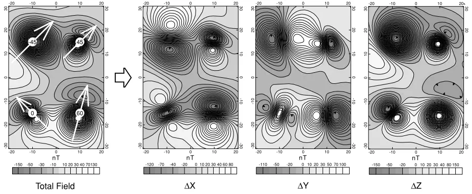
ΔX ΔY ΔZ
Fig. 1. The four-dipole example. The total field anomaly grid produced by four dipole sources having different magnetization directions (Total Field) is converted to magnetic component grids (X,Y,Z) by applying Fourier filters. The arrows represent the horizontal components of the magnetizations, the filled circles indicate the horizontal source locations, and the numbers in the circles indicate the inclinations of the magnetizations. The regional field has an inclination of 60◦and a declination of 15◦.
I5=
∞
−∞
∞
−∞xY d x d y=0
Furthermore (Helbig, 1963), the following integrals, repre-senting the remaining first order moments, should yield the average components of the magnetic dipole moment of the sources:
Here negative signs have been added to correct Helbig’s published equations for the case where the plane of integra-tion is above the sources andzis positive downward. Note that there are two estimates for the vertical component of the magnetic dipole moment,mz.
Because the total magnetization is parallel to the mag-netic dipole moment, it follows from (2) that the average magnetic dipole moment|m|, inclination im, and
declina-tiondmof the total magnetization are given by
|m| =m2
positive downward, anddmis positive clockwise from north
when viewed from above.
3.
Implementation
In order to apply Helbig’s equations to modern total field aeromagnetic data, we must first convert the gridded mag-netic data to vector component grids using Fourier filtering techniques (Lourenco and Morrison, 1973; Blakely, 1995, pp. 342–343). To do this, we only need to know the lo-cal geomagnetic field direction, which can be determined from models such as the International Geomagnetic Refer-ence Field (IGRF, Macmillanet al., 2003). Theoretically such transformations should only be applied to data that are measured on, or continued to a horizontal surface, but in practice this restriction is often ignored. Figure 1 shows this transformation for a four-dipole example, in which each of the dipoles has a different magnetization direction. This four-dipole example will be used to illustrate the approach of this paper.
Helbig’s four non-zero integrals (I6throughI9) are
Herexandyare the grid intervals, and the weightswi,j
take on the following values:
i = −n i =n
4 in window interior
2 on window edges 1 in window corners
(6)
In order to approximately satisfy Helbig’s vanishing in-tegrals (1), it was found to be necessary to remove best-fit planar surfaces fromX,Y, andZ within each small data window before integration. If (1) is not satisfied, the non-zero moments (2) will depend on the choice of origin. For example, ifx=x+x0,
which can only be satisfied if I1 = 0. Removing a mean
value from X, Y, and Z within each window will
assure that I1, I2, and I3are near zero. Removing a
best-fit planar surface within each window will help reduce the magnitudes ofI4andI5(Fig. 2).
Fig. 2. Chart showing how removing planar surfaces from the component grids prior to integration reduces the estimated magnitudes of Helbig’s vanishing integrals (I1throughI5) for the field of an isolated dipole .
IntegralsI1throughI3are not completely reduced to zero due to the
trapezoidal weighting used in the quadrature algorithm.
13 x 13
19 x 19
100 200 300 400 500 600 700 800 900 Am2
200 600 1000 1400 1800 2200 Am2
Fig. 3. Grids of moment, inclination, and declination of the magnetization for the four-dipole example as estimated using a 13×13 window and a 19×19 window. At the locations of the dipoles, shown by the black circles, the inclinations and declinations are correctly estimated.
4.
Two Methods
from different window sizes are in close angular agreement. This approach will be called the “direct” method, and is fur-ther subdivided into “basic” and “extended” versions. In the second approach, we seek grid nodes having solutions close to a specified magnetization direction, such as the inducing field direction. This will be called the “indirect” method.
4.1 The basic “direct” method
The basic “direct” method involves evaluating Helbig’s integrals using two different window sizes, finding the grid nodes where the angular differences between the two so-lutions are small, and calling these the best soso-lutions. The window sizes should be chosen to encompass representative isolated anomalies. Figure 3 shows grids of moment,
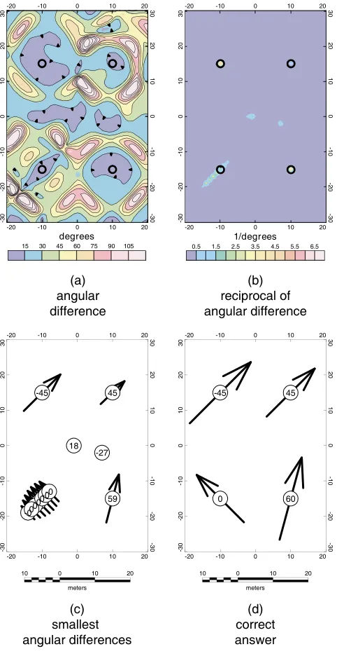
incli-Fig. 4. The basic “direct” method applied to the four-dipole example. (a) Angular difference between the results of the 13×13 window and the 19×19 window. Black circles indicate the dipole locations. (b) The reciprocal of the angular difference. (c) The magnetization solutions at the twelve grid nodes having the smallest angular differences. Symbols are as in Fig. 1. (d) The correct magnetizations.
nation, and declination of the magnetization as estimated using a 13 by 13 window and a 19 by 19 window on the four-dipole example, which has a grid cell size of 1 meter. Odd window sizes are used so the solutions can be assigned to the grid node at the center of the window. Overlapping windows provide solutions at all grid nodes, except near the edges of the data coverage. At the locations of the dipoles, shown by the black circles, the inclinations and declinations are estimated correctly. However, if the center of the win-dow is moved even slightly away from a dipole location, the estimated directions can be grossly inaccurate. Note that the estimated moments increase in magnitude as the window size increases.
Figure 4(a) shows the angular difference between the two solutions. Note that the difference is always low at the dipole locations. To emphasize this, Fig. 4(b) shows the reciprocal of the angular difference; the dipole locations are apparent. The southwest dipole is poorly located, probably because its magnetization is at approximately right angles to the regional field direction. The apparent solutions in the center of the area can be ignored, because they have very small moments.
Figure 4(c) shows the twelve solutions for the four-dipole example having the smallest angular differences. The cor-rect answer is in Fig. 4(d). Can we use Helbig’s integrals to estimate total magnetization directions? Figure 4 suggests that at least for semi-isolated dipoles the answer is “yes”.
4.2 The extended “direct” method
In an attempt to minimize the number of extraneous solu-tions, an extended version of the direct method was devel-oped. This involves generating solutions for many different pairs of window sizes using the basic direct method, and looking for clustering in the results. A cluster indicates re-peated solutions from different pairs of window sizes. For example, by using 12 odd window sizes varying from 3 by 3 grid nodes to 25 by 25 grid nodes, one can get 66 different pairs of window sizes as indicated by the circles in Fig. 5, leading to 66 different basic direct solutions.
The maximum allowable angular difference between
pairs of solutions must be adjusted for the difference in the size of the windows. The smallest maximum angular dif-ference is specified for solutions where the edges of the two windows differ by only two grid nodes (one “lag”). The allowable angular difference increases linearly as the dif-ference in window size increases, so that the maximum al-lowable angular difference between solutions from a 3×3 and a 25×25 window (eleven “lags”) is 11 times the max-imum angular difference between a 3×3 and a 5×5 win-dow. This linear relationship was chosen to approximately equalize the number of basic direct solutions for each pair of window sizes.
The estimated magnetic moment is also a function of window size, so the magnetic moments of the basic direct solutions are all normalized to the range of the moment
6.0 12.0 24.0 36.0 48.0 60.0
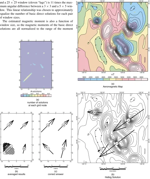
Fig. 6. Application of the extended direct method to the four-dipole example. (a) Number of basic direct solutions at each grid node having angular differences of one degree per lag or less. Any grid node can have from 0 to 66 solutions. (b) Averaged magnetization solutions for grid nodes having 40 or more solutions. (c) The correct magnetizations. The extended approach has removed the less reliable solutions of Fig. 4.
for the largest window at the end of processing. The win-dowed approach almost certainly provides poor estimates of the magnetic moments, even after this normalization. So the resulting magnetic moments should be considered rel-ative values rather than absolute values. In contrast, the
3800 4200 4400 4600 4800 5000 5200 5400 5600 6000
nT
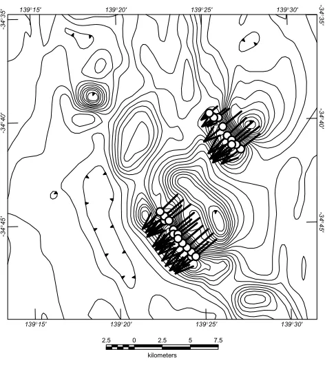
Fig. 7. The Black Hill Norite of South Australia is associated with the magnetic low in the northeast quadrant of the aeromagnetic map (a). A similar low appears to the southwest. The results of the extended direct method are shown in (b) and in Table 1. Aeromagnetic data
c
Table 1. Measured and estimated total magnetization directions for the Black Hill Norite, South Australia.
estimated inclinations and declinations are independent of window size and represent robust estimates of the total mag-netization direction.
Figure 6 shows the results of applying the extended direct method to the four-dipole example using the window sizes of Fig. 5. Any grid node can have from 0 to 66 solutions (Fig. 6(a)). The solutions are concentrated at the dipole locations. By averaging solutions for grid nodes having 40 or more solutions (Fig. 6(b)), the extended direct method has succeeded in eliminating the less reliable solutions in the center of the area (Fig. 4).
4.2.1 Example—Black Hill Norite, South Australia
Figure 7(a) shows a real-world example where the direct method works. This example was used by Schmidt and Clark (1997) for their Helbig analysis, and here an attempt has been made to reproduce their results. The Black Hill Norite is associated with the magnetic low in the northeast quadrant of the aeromagnetic map. A similar low appears 8.5 km to the southwest. The results of the extended direct method are shown in Fig. 7(b). Two bodies have large total magnetizations with southwest declinations and shallow up-ward directed inclinations. The results of the analysis can vary by a few degrees depending on how the clustering is
2.5 0 2.5
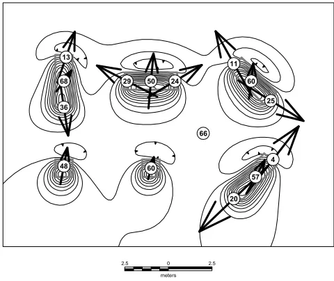
Fig. 8. Extended direct method results for a model consisting of six prisms, showing how horizontally elongated sources produce results that are accurate near their centers of mass (centers of dipole moment), but distorted near their ends. Basic direct method solutions were av-eraged at grid cells containing at least nine solutions; these avav-eraged solutions were then clustered within a radius of 0.75 meters, three times the grid interval.
done. Here basic direct solutions that agreed to within one degree per lag were averaged at grid nodes containing at least five solutions. These averaged values were then clus-tered using a radius of 5 kilometers. The grid interval was 400 meters.
Table 1 shows that the measured average total magnetiza-tion direcmagnetiza-tion for the Black Hill Norite is−20◦inclination and−131◦declination (Rajagopalanet al., 1993). Schmidt and Clark’s (1997) Helbig analysis resulted in a direction within 22◦ of the measured value. Results of the present study are even closer to the measured value (within 17◦and 10◦for the two bodies).
4.3 Elongated sources—a limitation of the “direct”
method
When the source bodies become elongated in the hor-izontal direction, the direct method starts to break down. Figure 8 shows extended direct method results for a model consisting of six prisms, five of which have dimensions of 1×1×3 meters, and one, in the bottom center, is a 1-meter cube. All prisms are magnetized in the direction of the geo-magnetic field, inclination 60◦, declination 15◦. Only the cube and the vertically elongated prism (lower left) give reasonable results. The horizontally elongated prisms pro-duce results that are accurate near their centers of mass (or centers of dipole moment), but distorted near their ends.
In the extreme case, where the magnetic bodies are so large or so elongated that any finite window will only see the body edges, the direct method will predict magnetiza-tions that are perpendicular to the body edges, as is illus-trated by a synthetic example of a pipeline over a buried fault (Fig. 9). Here the true magnetization direction is north. These results are not surprising. They are reminding us that for 2-D sources, we can really only estimate the component of the magnetization that is perpendicular to the strike di-rection.
In summary, the direct method allows the total magne-tization direction to be estimated from Helbig’s integrals without any a priori knowledge. But, it requires semi-isolated, compact source bodies without significant hori-zontal elongation, such as dipoles, spheres, or vertical cylin-ders.
4.4 The indirect method
2.5 0 2.5 5 7.5 meters
-136 -126 -113 -98 -90 -83 -76 -68 -61 -54 -46 -37 -13 10 27 40 50 58 64 70 75nT
Fig. 9. Extended direct method results (circles and arrows) for a model consisting of a magnetic field (graytone image) produced by a north-northeast-trending pipeline over a buried southeast-striking fault. For this extreme case of elongated magnetic source bodies, the method predicts magnetizations that are perpendicular to the body edges, be-cause for 2-D sources only the component of the magnetization that is perpendicular to the strike direction can be estimated. The true mag-netization direction is north. In this example, the maximum angular difference between lag-one solutions was taken to be 0.5◦, and a mini-mum magnetic moment of 2 ampere-meter2was used to reduce noise.
Results were clustered using a radius of 1 meter (5 grid intervals) and a minimum cluster size of two solutions.
identifying the grid nodes from the quadrature results where the estimated magnetization direction is close to a specified direction. If we again use twelve different window sizes for the quadrature analysis, then there will be from zero to twelve indirect-method solutions at each grid node. These solutions, like the direct solutions, can be thresholded, av-eraged, and (or) clustered to achieve a satisfactory result.
The goal of the indirect method is to identify the centers of mass (or centers of dipole moment) of sources that may have magnetization directions parallel to the specified di-rection. This goal is clearly met for the elongated prism ex-ample (Fig. 10), when the specified magnetization direction is chosen to be the inducing field direction. A comparison of Figs. 10 and 8 shows that the indirect method is much less sensitive to elongation of the sources than is the direct method.
In a second example, two likely sources of Black Hill
2.5 0 2.5
Fig. 10. Results of searching for all solutions within ten degrees of the inducing field direction for the elongated prism example. With twelve window sizes, each grid node can have up to twelve solutions. The results have been averaged at grid nodes having at least five solutions.
2.5 0 2.5 5 7.5
Fig. 11. Results of searching for all solutions within ten degrees of the measured total magnetization direction of the Black Hill Norite. Again only grid nodes having at least five of the twelve possible solutions are shown. Aeromagnetic data cCommonwealth of Australia (Geoscience Australia) 2003.
-347 -253 -222 -208 -197 -186 -177 -169 -161 -152 -142 -132 -123 -112 -99 -82nT
Fig. 12. Indirect method results for a Cenozoic volcanic center in the southern Albuquerque basin, New Mexico. Because the flows are Ceno-zoic, we know that the magnetizations are approximately parallel or anti-parallel to the present day geomagnetic field. Solutions that fall within 20 degrees of the geomagnetic field direction are shown, with white-filled symbols and south-directed arrows indicating reversed mag-netizations and black-filled symbols and north-directed arrows indicat-ing normal magnetizations. Clusterindicat-ing has been used to reduce the num-ber of solutions.
close to the Cenozoic direction.
This last example points out a possible ambiguity in the method. The reversely magnetized solutions are probably due to actual reversely magnetized rocks, but they could be due to zones of weaker normal magnetization within an otherwise strongly magnetized rock mass of normal polar-ity. Where the country rocks are strongly magnetized, it is important to remember that the magnetic anomalies are produced by magnetization contrasts rather than absolute magnetizations, so the estimated magnetization directions represent the contrasts (Schmidt and Clark, 1998).
5.
Conclusions
The Helbig integrals can be evaluated by quadrature anal-ysis in small data windows on magnetic component grids derived from total field magnetic anomaly data. Best-fit pla-nar surfaces must be removed from the component data in each small data window prior to integration. The windowed results provide local estimates of the moment, inclination, and declination of the total magnetization, which are valid near the centers of mass (centers of dipole moment) of the sources. By evaluating the integrals using several different window sizes, then comparing results from pairs of window sizes to find the grid nodes where the solutions are in close angular agreement, the source locations and the valid total magnetization directions can be identified. This “direct”
ap-proach works best for isolated, compact sources, and largely fails for horizontally elongated sources. An “indirect” ap-proach, in which the results from the different window sizes are searched to identify grid nodes where the estimated total magnetization is close to a specified direction, can always be used to locate sources having that magnetization direc-tion. In both the “direct” and “indirect” methods the scat-ter in solutions is reduced by specifying a minimum num-ber of solutions per grid node, averaging the solutions at grid nodes containing this minimum number, and option-ally clustering the averaged results within some radius.
Application of Helbig’s integrals should prove useful for rapid analysis of gridded aeromagnetic and ground mag-netic anomaly data. The “direct” method should be par-ticularly valuable for locating the centers of mass (centers of dipole moment) and in characterizing the total magne-tization directions of both localized geologic bodies such as small plutons, volcanic centers, and kimberlite pipes, and localized cultural sources such as well casings, buried drums, and unexploded ordnance.
The “indirect” method should be useful for locating the centers of mass (centers of dipole moment) of magnetic sources having a specified total magnetization direction. For example, by specifying the inducing field direction, bodies having predominantly induced magnetization can be located, and, by exclusion, bodies having significant rem-anant magnetization can be identified. By specifying a mea-sured total magnetization direction, multiple bodies having the same geologic age and magnetic properties can be iden-tified (e.g., the Black Hill Norite). Source bodies having primarily remanent magnetization, such as volcanic flows, can be located by specifying normal and reversed magneti-zation directions for rocks of that particular geologic age.
Acknowledgments. This paper was presented at the 2003
Inter-national Union of Geodesy and Geophysics (IUGG) meeting in Sapporo, Japan, and it incorporates aeromagnetic data which is:
c
Commonwealth of Australia (Geoscience Australia) 2003. The author is grateful to Phillip Schmidt and David Clark for rediscov-ering Helbig’s paper and demonstrating the practical value of his equations through published results on Australian aeromagnetic data. A discussion with Dr. Schmidt at his 2002 European Geo-physical Society poster presentation prompted the research that led to this paper. The author also thanks Rick Saltus and Bruce Smith for thoughtful reviews of an early draft, Rick Blakely and David Clark for helpful reviews of the submitted manuscript, and Yaoguo Li for pointing out the sign error in Helbig’s published integrals.
References
Bhattacharyya, B. K., A method for computing the total magnetization vector and the dimensions of a rectangular block-shaped body from magnetic anomalies,Geophysics,31, 74–96, 1966.
Blakely, R. J.,Potential Theory in Gravity and Magnetic Applications, Cambridge University Press, Cambridge, 441 pp., 1995.
Emilia, D. A. and R. L. Massey, Magnetization estimation for nonuni-formly magnetized seamounts,Geophysics,39, 223–321, 1974. Helbig, K., Some integrals of magnetic anomalies and their relation to the
parameters of the disturbing body,Zeitschrift f¨ur Geophysik,29(2), 83– 96, 1963.
Lourenco, J. S. and H. F. Morrison, Vector magnetic anomalies derived from measurements of a single component of the field,Geophysics, 38(2), 359–368, 1973.
generation International Geomagnetic Reference Field released,EOS, Transactions, American Geophysical Union,84(46), 503, 18 November 2003.
McCracken, D. D. and W. S. Dorn,Numerical Methods and Fortran Pro-gramming, John Wiley and Sons, Inc., New York, 457 pp., 1964. Mederios, W. E. and J. B. C. Silva, Simultaneous estimation of total
magnetization direction and 3-D spatial orientation,Geophysics,60(5), 1365–1377, 1995.
Parker, R. L., L. Shure, and J. A. Hildebrand, The application of inverse theory to seamount magnetism,Rev. Geophys.,25, 17–40, 1987. Rajagopalan, S., P. Schmidt, and D. Clark, Rock magnetism and
geophysi-cal interpretation of the Black Hill Norite, South Australia,Exploration Geophysics,24, 209–212, 1993.
Rao, B. S. R., T. K. S. Prakasa Rao, and A. S. Krishna Murthy, A note on magnetized spheres,Geophys. Prosp.,25, 746–757, 1977.
Schmidt, P. W. and D. A. Clark, Directions of magnetization and vector anomalies derived from total field surveys,Preview,70, 30–32, 1997. Schmidt, P. W. and D. A. Clark, The calculation of magnetic components
and moments from TMI: A case history from the Tuckers igneous com-plex, Queensland,Exploration Geophysics,29, 609–614, 1998. Schnetzler, C. C. and P. T. Taylor, Evaluation of an observational method
for estimation of remanent magnetization,Geophysics,49, 282–290, 1984.
U.S. Geological Survey and Sander Geophysics, Ltd., Digital data from the Isleta-Kirtland aeromagnetic survey, collected south of Albuquerque, New Mexico,U.S. Geological Survey Open-File Report 98-341 (CD-ROM), 1998.