A New Model Transfer Mechanism Framework for
1
SLEUTH Model Performance Evaluation
2
Fang Liu 1,2, Jinling Quan 3,4, Ling Zhu 1,2, Qiang Chen 1,*, Yizhou Meng 1, Zhechen Na 1,
3
Yanfang Li 1, Ang Gao 1, Sinan Li 1
4
1 School of Geomatics and Urban Spatial Information, Beijing University of Civil Engineering and
5
Architecture, Beijing 100044, China; [email protected] (F.L.); [email protected] (L.Z.);
6
[email protected] (Q. C.); [email protected] (YZ. M.); [email protected] (ZC.N.);
7
[email protected] (YF.L.); [email protected] (A.G.); [email protected] (SN.L.)
8
2 Key Laboratory for Modern Urban Surveying and Mapping of National Administration of Surveying,
9
Mapping and Geoinformation, Beijing 100044, China;
10
3 Institute of Geographic Sciences and Natural Resources Research,CAS, Beijing 100101, China;
11
[email protected] (JL.Q)
12
4 State Key Laboratory of Resources and Environmental Information System;
13
* Correspondence: [email protected]; Tel.: +86-152-1098-0906
14
Abstract: SLEUTH Model (slope, landuse, exclusion, urban extent, transportation and hillshade) is
15
an important tool for landuse planning and land policy. To evaluate the performance of SLEUTH
16
model, implementation of Sensitivity Analysis (SA) is essential. The main limitation of SA in
17
SLEUTH application is a lack of insight into model input self-modification parameters (SMPs)
18
variation, namely, uncertainty involved in the model transfer metrics and model presumptions,
19
which often misled the decision makers and model users. To address this issue, this study divided
20
the forward process into two stages. Firstly, during the transfer process ①, the contribution scores
21
of five SMPs were drawn, and parameters highly sensitive to model output were given. Apart from
22
that, the recommended initial value for SMPs of 0.11, 0.2, 0.87, 1.13, 15, 1.01, 0.49 were found to be
23
subordinated to such a heterogeneous urban area simulation. Secondly, during the transfer process
24
②, SMP caused imagery metrics indicated the disparity between parameters with Fixed Reference
25
and with Successive Reference. Reversely, it derives reasonable threshold for the best fit values of
26
five prediction coefficients’ initialization by comparing the real image with the predicted one. The
27
framework of SLEUTH model transfer mechanism not only could distinguish highly sensitive SMPs
28
with higher contribution scores, but also could give parametric analysis for simulation imagery
29
based on metrics. The study was found to be a practical tool for quantization response of model
30
input variables for modelling complex urban systems. So, this insight can help geographic
31
information scientists decide how to find out the inner forward transfer mechanism of SLEUTH
32
model for further make good use of it and improve the model.
33
Keywords: SLEUTH model; Sensitivity Analysis; uncertainty assessment; urban expansion
34
35
1. Introduction
36
SLEUTH models (slope, landuse, exclusion, urban extent, transportation and hillshade) of
37
landuse change are popular and useful tools for simulating complex urban systems (e.g. Andreas
38
Rienow & Roland Goetzke, 2015; Anıl Akın et al., 2014; Gargi Chaudhuri & Keith C. Clarke, 2014;
39
Javad Jafarnezhad et al., 2016; Mahesh Kumar Jat et al., 2017; Haiwei Yin, 2016). A review on the
40
SLEUTH land use change model was published in paper (Gargi Chaudhuri & Keith Clarke, 2013).
41
However, morphology and structure form of urban sprawl are full of variety, considering
42
urbanization has hastened the process in region land use. Meanwhile the urbanization model
43
research is always a hot issue for geographical scientists. Paper “Urban growth models: progress and
44
perspective” (Xuecao Li & Peng Gong, 2016) researched hundreds of models and abstracted the
45
evolution of urban growth models from two perspectives: from macro to micro, from static to
46
dynamic (Xiping Cheng & Hu Sun, 2012; Na Li, 2011; Chi Xu, 2015). Besides, this paper outlined “An
47
evolution tree of CA-based urban growth models” according to importance dimension and age
48
dimension. At present, these models developed in terms of modeling mechanisms, data-driven
49
mechanisms (based on statistical empirical relationships) and process-driven approach mechanisms
50
(based on feedback and interactions). A kind systematic retrospect model is needed for future new
51
model development.
52
Sensitivity analysis (SA) represents an important step in improving the understanding and use
53
of landuse change prediction models. The results inaccuracies and uncertainty of model might be
54
attributed to the structure and nature of model, SA is the only critical tool for quantifying response
55
of model input variables for modelling complex urban systems, and avoiding unusually high or low
56
growth rate of urban expansion. There are many different SA approaches. Overall, they can be
57
categorized into two groups: local SA and global SA. The local SA explores the changes of model
58
response by varying one parameter while keeping other parameters constant. The simplest and most
59
common approach is differential SA (DSA), which uses partial derivatives or finite differences of
60
parameters at a fixed parameter location as the measure of parametric sensitivity. On the other hand,
61
the global SA examines the changes of model response by varying all parameters at the same time,
62
allowing them to provide robust measures in the presence of nonlinearity and interactions among
63
the parameters (Haruko M.Wainwright, 2014), and thus are generally preferred due to their global
64
properties (Andrea Saltelli, 2008). Generalized SA (GSA) method is one of the global SA methods that
65
are designed to overcome the limitations of local SA methods. A version of GSA method, the
66
Generalized Likelihood Uncertainty Estimation (GLUE) method was developed (Keith Beven &
67
Andrew Binley, 1992). GSA is simple to implement and can work with different pseudo-likelihood
68
(i.e., goodness of fit) measures (Keith J. Beven, 2011), but it is computationally inefficient.
One-At-a-69
time (OAT) approach have gained popularity recently because they offer the most representative
70
local sensitivity measures while maintaining computational efficiency. In sum, the complexity of
71
these problems highlights the need to understand the sources and range of uncertainty associated
72
with different aspects of the modeling process ( Erqi Xu & Hongqi Zhang, 2013; Amin Tayyebi et al.,
73
2016). Because it is easy to implement, computationally inexpensive, and useful to provide a glimpse
74
at the model behavior. Recently, Jiri Nossent & Willy Bauwens (2012) adopted the OAT method for
75
parameter SA of the Soil and Water Assessment Tool (SWAT) model, considering three values for
76
each of the seven parameters. By exploring three values for each of the two factors, Zoras et al. (2007)
77
conducted a parameter screening experiment based on the OAT method for an air pollution model.
78
SA for Cellular Automata urban land use model have been done by someone (Verda Kocabas &
79
Suzana Dragicevic, 2006; Hossein Shafizadeh-Moghadam et al., 2017; Richard Hewitt &
JaimeDíaz-80
Pacheco, 2017). However, as a popular and important method derived from it (Xuecao Li &Peng
81
Gong, 2016), SA for SLEUTH has not been recorded yet.
82
In this paper, two issues would be dealt with. Forwardly, by means of SA, modelers may probe
83
the response relationship between independent variables and dependent variables using sample data,
84
and discriminate important model factors from non-influential model factors. Reversely, it derives
85
reasonable threshold for the best fit values of five prediction coefficients’ initialization for predicting
86
the real images. These questions are addressed by OAT SA method using sample image data from
87
SLEUTH3.0beta_p01 LINUX released 6/2005 sponsored by Project Gigalopolis, downloaded from
88
website: http://www.ncgia.ucsb.edu/projects/gig/Dnload/download.htm.
89
2. Materials and methods
90
2.1. SLEUTH model & Data
91
SLEUTH is characterized by a series of rules in a nested loop to simulate urban growth, that
92
derived by four growth rules as follows (Matteo Caglioni et al., 2006; Keith Clarke, 2008; AnılAkın,
93
2014): 1) the spontaneous growth defines the probability for any non-urbanized cell to be developed
94
into an urban cell in the next step, which is determined by the diffusion and slope parameters; 2) the
95
new spreading center growth defines the probability that the new, spontaneously urbanized cells will
96
become new urban spreading centers, which is determined by the breed and slope parameters; 3) the
97
edge growth defines the probability for existing urban spreading centers to expand outward or
98
inward, which is determined by the spread and slope parameters; and 4) the road influenced growth
simulates the tendency of new urban cells to appear near existing transportation networks, which is
100
determined by the breed, road gravity, diffusion, and slope coefficients.
101
SLEUTH uses a brute-force method, making attempts on sufficient combinations of model
self-102
modification parameters (SMPs) to perform a calibration and derive a set of parameters that can best
103
capture the historic growth trend of a study area. The SMPs includes seven parameters as:
104
ROAD_GRAV_SENSITIVITY, SLOPE_SENSITIVITY, CRITICAL_LOW, CRITICAL_HIGH,
105
CRITICAL_SLOPE, BOOM, BUST. These initial empiric values setting decide the processing
106
and final results; at the same time, and govern the urban simulation imagery. If there is one real
107
imagery, new initial value could simulate “Ideal imagery” with no significant discrepancy with real
108
one.
109
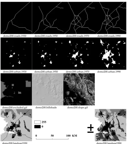
Tested object is demo200 image package download along with “SLEUTH3.0beta_p01_linux”,
110
which is dependent of model input parameters SA test. Figure 1 illustrates the input maps in 1m
111
resolution with size of 200×200.
112
demo200.roads.1930 demo200.roads.1950 demo200.roads.1970 demo200.roads.1990
demo200.urban.1930 demo200.urban.1950 demo200.urban.1970 demo200.urban.1990
demo200.excluded.gif demo200.hillshade demo200.slope.gif
demo200.landuse1930 demo200.landuse1990
Figure 1. The input maps of demo200 with size of 200×200
113
255 0
Figure 1 illustrates the construction of SLEUTH model input image. In figure 1, it is consisted of
114
six types of data as: slope, landuse, exclude, urban, roads and hillshade, respectively.
115
2.2. Simulation workflow design
116
In the forward stage, three goals were accomplished.
117
1) The Processing results response to the Initialization parameters variation have been
118
recorded and a new rule was established.
119
2) The Final results response to the Initialization parameters variation have been recorded
120
and the above rule was supplemented.
121
3) An important Feedback mechanism from the rules for monitoring the control governance
122
was extracted.
123
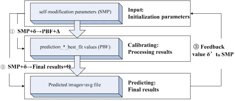
The forward simulation workflow govern by SMPs is combined by three stages (in Figure 2):
124
firstly, little alteration to SMPs has transmitted corresponding information to PBFs, which is called
125
stage ①: SMP+δ→PBF+Δ; secondly, little alteration to SMPs has acted on predicted images and avg
126
files indirectly, which is called stage ②: SMP+δ→Final results+Θ. thirdly, new alteration value δ‘ is
127
drawn from the feedback mechanism, which is called stage ③.’
128
129
Figure 2. Workflow chart of SLEUTH Simulation framework
130
SMP is the initial empiric value setting, which is expressed as {Ni, i=1,2,3,4,5,6}. The coefficients
131
effect how the growth rules are applied to the data. They are, N1: ROAD_GRAV_SENSITIVITY, N2:
132
SLOPE_SENSITIVITY, N3: CRITICAL_LOW, CRITICAL_HIGH, N4: CRITICAL_SLOPE, N5:
133
BOOM, N6: BUST respectively. One suite of parameter set only with one δ alteration added
134
upon one Ni parameter, expressed as {N1, N2, …, Ni+ δ,i …N6}. There are 65 suite of parameter sets
135
totally, as one suitable alteration added to one each time.
136
PBF is the processing best fit record by altering the suite of parameter set calculated from the
137
four steps calibration, which is expressed as {Gk, k=1,2,3,4,5}. They are, G1:
138
PREDICTION_DIFFUSION_BEST FIT, G2: PREDICTION_SPREAD_BEST_FIT, G3:
139
PREDICTION_BREED_BEST_FIT, G4: PREDICTION_SLOPE_RESISTANCE _BEST_FIT, G5:
140
PREDICTION_ROAD_GRAVITY _BEST_FIT. PBF, which is purposed to predict the final images
141
and record, is inseparably related with SMP. In order to detect the SA details, different relationship
142
expression strategies are applied. It employed: 1) Weight; 2) absolute value; 3) difference unitization
143
using the initial empiric value; 4) difference unitization using the sorting values.
144
The final results are including: Predicted images and avg files, which are the indirect result from
145
PBF, which is also the record of model input parameters set SMPs varying. Prediction images are
146
landuse charts from 1991 to 2010, totally twenty years. Considering too many images, 20*65,
147
simplified metrics are borrowed for measuring charts. They are, M1: Error Ellipse, M2: Clusters
148
Aggregation, M3: Urban Area percentage, M4: Roads’ correlationship with urban. The alteration of
Final chart is expressed as {M1+ Θ1, M2+ Θ2, …, Mj+ Θj, …M4+ Θ4}. As for avg files, they are coefficients
150
record which decides how the growth rules are applied year by year.
151
2.3. Experiment set up: Model parameters initialization and variation design
152
The initial states setup of model were parameters {Ni} with experience values. However, this
153
paper tends to explore the model with different initial states set different values, which could be
154
applied to heterogeneous urban area simulation. The initial model parameters are experience values
155
included along with SLEUTH code, supplied by original authors. They are, N1:
156
ROAD_GRAV_SENSITIVITY=0.01, N2: SLOPE_SENSITIVITY=0.1, N3: CRITICAL_LOW=0.97,
157
CRITICAL_HIGH=1.03, N4: CRITICAL_SLOPE=15, N5: BOOM=1.01, N6: BUST=0.09.
158
The aim of variation design is to make a clear of model dynamic transmission mechanism from
159
beginning to the end. According to the idea of OAT sensitivity analysis methodology, this paper
160
measures both system sensitivity and system result response to each independent parameter
161
variation with different size and tendency. There are seven parameters divided into six groups,
162
considering N3 consisting of CRITICAL_LOW and CRITICAL_HIGH, which are widened or
163
narrowed simultaneously. There are altogether six groups of initial input parameters are controlled,
164
and 65 experiment suites are recorded. One parameter suite with only one δ alteration to one
165
parameter, the minimum step size is set to 0.02 or 0.2 (CRITICAL_SLOPE only), while the study
166
ranges as ±100 times. Considering their physical meaning, there are 65 experiment suites are
167
produced induced from six groups of initial input parameters with range of variable from minus to
168
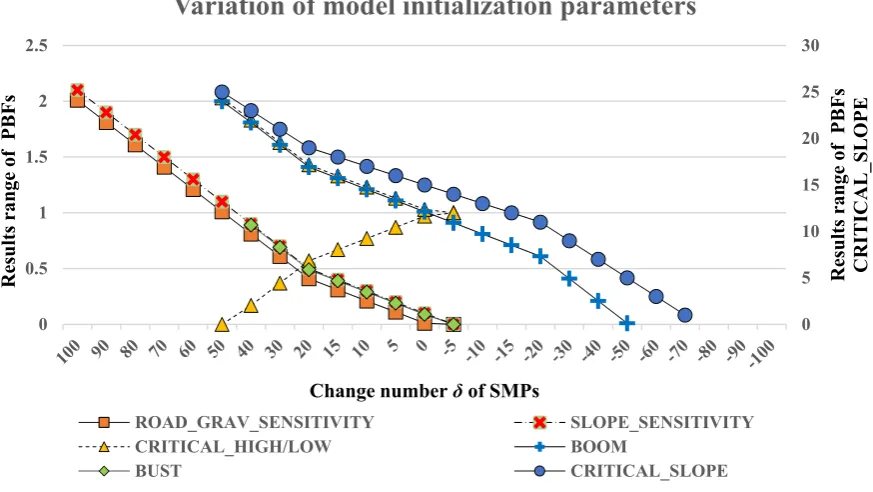
positive (Figure 3, Table 1).
169
170
Figure 3. Variation of model initialization parameters (in chart form). X axis stands for increment
171
change δ of SMPs, and Y axis are double axes, standing for dependent variable Δ for PBFs, where,
172
left axis indicating all PBFs results range except CRITICAL_SLOPE, right axis indicating PBFs results
173
range of CRITICAL_SLOPE.
174
2.4. Two Derivatives from Absolute Value
175
When SA information mining is dealed with, two derivatives from Absolute Value are
176
developed, First Difference to fix reference and First Difference to relative reference(formula (1)-(2)).
177
First Difference to fix reference is applied for analysing the differences (Δ) between the output
178
predicted maps/data and standard reference map, the latter with no change on control parameters
179
set. Additionanlly, First Difference to successive Referenceis used for evaluating the differences (Δ)
180
0 5 10 15 20 25 30
0 0.5 1 1.5 2 2.5
Results
range
of PBFs
CRITICAL_S
LOPE
Results
range
of PBFs
Change number δof SMPs
Variation of model initialization parameters
ROAD_GRAV_SENSITIVITY SLOPE_SENSITIVITY
CRITICAL_HIGH/LOW BOOM
between two consecutive output predicted maps/data. In order to unify the rate of output results
181
variation, the above-mentioned differences (δ) have both been dividied by the change of input
182
parameter (Δ). The expression formulars are:
183
= | | , (1)
= | | , (2)
where, SMP+δ is expressed as{N1, N2, …, Ni+ δ,i …N6}; PBF+Δ is expressed as{G1+Δ1, G2+Δ2, …,
184
Gk+Δk …G5+Δ5};
185
i is {Ni, i=1,2,3,4,5,6}, which decides which SMPs to deal with.
186
δ, δ' are change of input parameter which are controlled, which means δor δ' times of 0.02 (or
187
0.2 for CRITICAL_SLOPE only) added to the reference values.Δ is change of PBFs caused by δ, δ'.
188
First Difference to fix reference ( ): its role is to reflect where the initial empirical value is
189
located properly on the X axis.
190
First Difference to Successive reference ( ): its role is to reflect the difference of response
191
between adjacent points has any relationship with location of X.
192
2.5. Charts Metrics
193
In order to evaluate the geographical expansion of cities, from the predicted imagery. four
194
evaluation indicators are employed, as Directional Distribution, Clusters Aggregation, Urban Area
195
percent, Roads’ correlationship with urban, respectively (Table 1).
196
Table 1. Metrics for imagery
197
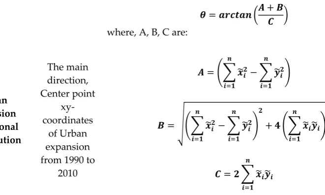
Indices Description Formula
Urban expansion Directional Distribution
The main direction, Center point
xy-coordinates
of Urban expansion from 1990 to
2010
θ is the azimuthal orientation angle with due North. The
rotation angleθ is calculated as:
= +
where, A, B, C are:
= −
= − +
=
where and are the derivations of the xy-coordinates from
the Mean Center.
= ∑ −
where xi and yi are the coordinates for feature i, { , }represents
the Mean Centre for the features, and n is equal to the total
number of features
Urban Clusters Aggregation
Urban spatial aggregation
degree in 2010
= √ /
where A: Urban Clusters Area, P:Urban Clusters Perimeter
Urban Area percent /%
Urban proportion
in 2010
= /
where A: Urban Expansion Area; AT:Imagery total Area
Correlationship between Existed Road &
Simulated Urban Imagery
Correlation between road buffer in 1990 & urban in 2010
= ∑ − −
∑ − ∑ −
where xi:Urban pixel value; yi: Road pixel value; , : the
average value of cluster values of xi, yi
3. Results
198
In order to detect the SA details, process record and final graphic and data results are carried
199
out quantitative analysis with input model parameters. Two research tasks were done.
200
1)The biggest contributors are screened out and sorted in descending order by the Weight
201
values. Meanwhile, the volatility features of trend are described by the Absolute Value curve.
202
2)Evaluate whether the initial empiric value setting is appropriate one for each index.
203
demo_land_urban.1995 demo_land_urban.2000 demo_land_urban.2005 demo_land_urban.2010
Figure 4. The output predicted landuse maps and the growth types of demo200
204
Figure 4 depicts the predicted maps derived from the above input image for simulations. The
205
Legends clearly shows LANDUSE CLASS and GROWTH TYPE.
206
3.1 Model PBF Response to SMP variations
207
There are two types of data as the Model PBF Response results to SMP variations, Weight
(0-208
100%) and Absolute Value (0.00-100.00). Table 2 illustrate the stage ① in figure 2, that is, six groups
209
input model parameters variation and the corresponding Model PBF Responses, including:
210
ROAD_GRAV_SENSITIVITY, SLOPE_SENSITIVITY, CRITICAL_ HIGH/ LOW, CRITICAL_SLOPE,
211
BOOM and BUST. Interval of independent variable is set to be regular pattern, and the fine distinction
212
caused by model initialization parameters A-F series variation are studied.
213
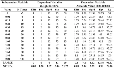
Table 2. ROAD_GRAV_SENSITIVITY index series variations and the corresponding Model PBF Response
214
Independent Variable Dependent Variable Dependent Variable
Weight (0-100%) Absolute Value (0.00-100.00)
Value N Times Diff Brd Sprd Slp Rg Diff Brd Sprd Slp Rg
0 -5 1 1 12 75 30 1.78 1.78 21.38 39.73 30
0.01 0 1 1 12 80 1 1.79 1.79 21.37 44.8 4.53
0.11 5 1 3 12 75 30 1.79 5.34 21.37 38.44 70.21
0.21 10 1 1 12 75 28 1.79 1.79 21.37 39.68 99.01
0.31 15 1 2 10 75 16 1.7 3.4 16.78 44.7 93.07
0.41 20 1 3 12 83 30 1.76 5.31 21.17 46.97 98.02
0.61 30 1 5 12 79 17 1.78 8.91 21.38 41 99.01
0.81 40 1 2 12 79 4 1.78 3.57 21.37 43.08 99.01
1.01 50 1 1 12 73 15 1.8 1.8 21.58 36.8 100
1.21 60 1 1 10 79 17 1.73 1.73 17.11 48 95.05
1.41 70 1 1 10 79 8 1.71 1.71 16.76 49.12 93.07
1.61 80 1 1 12 84 1 1.76 1.76 21.16 49.26 98.02
1.81 90 1 1 14 83 10 1.8 1.8 25.18 44.15 100
2.01 100 1 1 12 79 1 1.78 1.78 21.38 43.29 99.01
RANGE 0 4 4 11 29 0.1 7.2 8.42 12.46 95.47
STDEV 0.00 1.20 1.07 3.44 11.22 0.03 2.14 2.29 3.98 29.76
Note: Diff, Brd, Sprd, Slp, Rg are abbreviation forms of DIFFUSION, BREED, SPREAD, SLOPE_RESISTANCE,
215
ROAD_GRAVITY.
216
Table 2 shows that one of six groups input model parameters variation and the corresponding
217
Model PBF responses.
218
(a) SLOPE_SENSITIVITY (a)
ROAD_GRAV_SENSITIVITY
(c) CRITICAL_LOW/ CRITICAL_HIGH
(d) CRITICAL_SLOPE (e) BOOM (f) BUST
Figure 5. SMP indices variations and the corresponding Model PBF Response in Weight form
219
From the Figure 5, the weight ranges of SMP indices variations are shown. The following table
220
summarizes their behavior and lists them in sensitivity degree rank, which explains how much SMPs
221
variation δ contribute to the PBF alteration Δ.
222
Table 3. Sensitivity Rank of Dependent Variables’ Weight
223
Dependent Variable
Weight (0-100%)
Sensitivity degree
(%) Diff Brd Sprd Slp Rg
80-100
60-80 √ √
40-60
20-40 √
0-20 √ √
Average STDEV 1.62 4.21 2.88 13.05 15.99
Average Range 4.42 13.66 8.78 44.91 38.54
From Table 3, the weight ranking of the SMPs for all criteria is as follows:
224
(SLP,GR)>BRD>(DIFF,SPRD). SLP and GR which are assigned weight of 60%~80%, are
high-225
sensitivity indices. Similarly, BRD are low sensitivity index, while DIFF and SPRD are extrem low
226
sensitivity indices.
227
First Difference to a fixed Reference is used to reflect where the initial empirical value is located
228
properly on the X axis, while First Difference to a Successive Reference method is employed to
229
judge the difference of response between adjacent points has certain relationship with location of X.
230
231
232
233
-20 0 20 40 60 80 100 120 2.011.81 1.61 1.41 1.21 1.01 0.81 0.61 0.41 0.31 0.21 0.11 0.01 0 Diff Brd Sprd Slp RG ROAD_GRAV_SENSITIVITY -20 0 20 40 60 80 100 120 2.1
1.9 1.7 1.5 1.3 1.1 0.9 0.7 0.5 0.4 0.3 0.2 0.1 0 Diff Brd Sprd Slp RG SLOPE_SENSITIVITY -20 0 20 40 60 80 100 120 0 0.17 0.37 0.57 0.67 0.77 0.87 0.97 1 Diff Brd Sprd Slp RG CRITICAL_LOW_HIGH 0 20 40 60 80 100 120 25 23 21 19
18 17 16 15 14 13 12 11 9 7 5 3
1 Diff
Brd Sprd Slp RG CRITICAL_SLOPE 0 20 40 60 80 100 120 2 1.81 1.61 1.41 1.31 1.21 1.11
1.01 Diff
Brd Sprd Slp RG BOOM 0 20 40 60 80 100 120 0.89 0.69 0.49 0.39 0.29 0.19 0.09
0 Diff
Brd Sprd Slp RG
Compare to a Fixed Reference in Line Plot (Fluctuation/Trend)
Compare to a Successive Reference in Radar Plot (Dispersion)
-10 -5 0 5 10 15
1.81
1.61
1.41
1.21
1.01
0.81 0.61
0.41 0.31
0.21 0.11 0.01
0 Diff
Brd Sprd Slp RG SMP variations to ROAD_GRAV_SENSITIVITY
-10 -5 0 5 10
1.9
1.7
1.5
1.3
1.1
0.9 0.7
0.5 0.4
0.3 0.2 0.1
0 Diff
Brd Sprd Slp RG SMP variations to SLOPE_SENSITIVITY
-10 -5 0 5 10
0.17
0.37
0.57
0.67
0.77 0.87 0.97
1 Diff
Figure 6. SMP indices variations and the corresponding Model PBF Response in difference form
234
In Figure 6, When SA details of stage ① are explored, two chart forms as First Difference to a
235
fixed Reference of SMP indices variations are employed, line plot and radar plot. Line plot is applied
236
for exploring the rules of trend and fluctuation as each input parameter is ascending. As a
237
supplement, radar plot is used to observe the dispersion of each series variation, as well as outliers‘
238
position.
239
According to the First Difference to the Fixed Reference results, the trend line of
240
RD,SLP,BREED and SPREAD have inflexion points in the known empirical value x=0.11, namely,
241
ascending before the point, descdending after that point. Generally speaking, considering
242
parameters‘ weight, the recommended initial value located on the X axis should be 0.11 for
243
ROAD_GRAV_SENSITIVITY index.
244
-10 -8 -6 -4 -2 0 2 4 6 8
23
21
19
18
17
16
15
14 13
12 11
9 7 5 3
1 Diff
Brd Sprd Slp RG SMP variations to CRITICAL_SLOPE
-10 -5 0 5 10
--1.81
1.61
1.41
1.31 1.21 1.11
1.01 Diff
Brd Sprd Slp RG SMP variations to BOOM
-10 -5 0 5 10
--0.69
0.49
0.39
0.29 0.19 0.09
0 Diff
Still the same method, the appropriate values of four SMPs is set as 0.2, 0.87, 1.13, 15, 1.01, 0.49
245
respectively, compared with the original empirical value at 0.1, 0.97, 1.03, 15, 1.01, 0.09, for
246
SLOPE_SENSITIVITY, CRITICAL_LOW/HIGH, CRITICAL_SLOPE, BOOM, BUST, respectively
247
(Table 4).
248
Table 4. Sensitivity Rank of Dependent Variables’ Weight
249
ROAD_G RAV_SEN SITIVITY
SLOPE_S ENSITIVI
TY
CRITICA L_LOW_ HIGH
CRITICA
L_SLOPE BOOM BUST
Empirical
Value Location 0.01 0.1 0.97,1.03 15 1.01 0.09
Appropriate
Value Location 0.11 0.2 0.87,1.13 15 1.01 0.49
Change Value +0.10 +0.10 -0.10,+0.10 0 0 +0.40
According to the First Difference to a Successive Reference results, conclusion from figure 6 is
250
drawn: for different initialization parameters, the sensitive position of the same PBF parameter are
251
different, which proved that specific position has certain relationship with sensitivity extent.
252
According to the radar diagram, the positioin sensitive point of ROAD_GRAV_SENSITIVITY is 0.01.
253
Still the same method, the positioin sensitive point to PBF parameter are set as 0.77, 1 and 0.39 in
254
CRITICAL_LOW/HIGH, CRITICAL_SLOPE, BUST, while SLOPE_SENSITIVITY and BOOM indics
255
keep stationary situations.
256
3.2 Model Imagery Response to SMP variations
257
In this part, output predicted imagery and its imagery description indices results are discussed.
258
Considering too many output predicted images (in Figure 3), 20*65, simplified metrics are borrowed
259
for measuring charts. They are, six groups input model parameters variations and the corresponding
260
Model Imagery indices Responses results, including: Directional Distribution, Clusters Aggregation,
261
Urban Area percent, Roads’ correlationship with urban, respectively (Table 1).
262
Figure 7 (a) – (d) illustrate the four groups input model parameters variation and the
263
corresponding model imagery metrics ‘responses.
264
265
±
σ=18.4°
±
σ=20.6°
±
Figure 7(a). Imagery metrics for Model PBF Response in difference form. Urban expansion Directional
266
Distribution Index indicates the main direction of Urban expansion from 1990 to 2010. From the
267
figures above, the Directional Distribution Index are 18.4° to 33.8° from the due North.
268
±
σ=27.7°
±
σ=31.5°
±
σ=33.8°
Raster_DirectionalDistribution Non Urban
Urban
0 50 100 KM
±
±
Average Aggregation Index=0.8148
±
Average Aggregation Index=0.8293
±
Average Aggregation Index=0.8301
±
Average Aggregation Index=0.8365
±
Average Aggregation Index=0.8411
±
Average Aggregation Index=0.8452
±
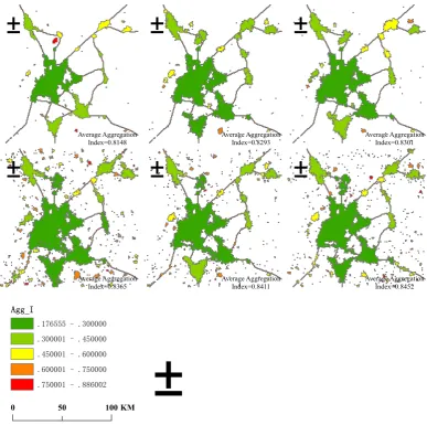
Agg_I
.176555 - .300000
.300001 - .450000
.450001 - .600000
.600001 - .750000
.750001 - .886002
Figure 7(b). Imagery metrics for Model PBF Response in difference form. Urban Clusters Index
269
indicates the urban patches spatial aggregation degree in 2010 predicted imagery. From the figures
270
above, the Average Aggregation Index are 0.8148 to 0.8452, .reflecting a certain degree of clustering
271
tendency.
272
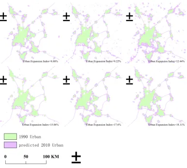
Figure 7(c). Imagery metrics for Model PBF Response in difference form. Urban Area percent Index
273
indicates the urban proportion in 2010 predicted imagery. From the figures above, the Urban Area
274
percent Index are 8.88% to 18.11%, .reflecting a relative proportion of urban cover area.
275
±
Urban Expansion Index=8.88%
±
Urban Expansion Index=9.22%
±
Urban Expansion Index=12.44%
±
Urban Expansion Index=15.06%
±
Urban Expansion Index=17.6%
±
Urban Expansion Index=18.11%
±
1990 Urban
predicted 2010 Urban
0 50 100KM
±
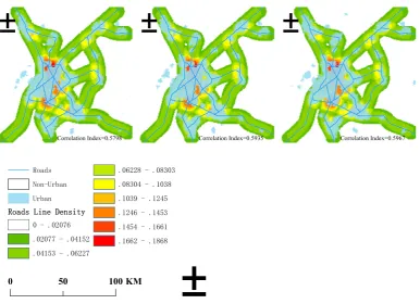
Correlation Index=0.5360
±
Correlation Index=0.5513
±
Figure 7(d). Imagery metrics for Model PBF Response in difference form. Correlationship between
276
Existed Road & Simulated Urban Imagery Index indicates the Correlation between road buffer in 1990
277
with urban in 2010 predicted imagery. From the figures above, the Correlation Index are from 0.5360
278
to 0.5967, .reflecting a significant correlationship.
279
From stage ② the relation between SMPs and Final results (imagery indices) could be
280
established as follows:
281
× = , (3)
where, N is SMP variation groups of {Ni, i=1…6}, M is the Final imagery response groups of {Mj,
282
j=1…4}. X stands for the transition relationship from SMP to imagery variation, which is what we
283
need to explain the quantitative transition mechanism of stage ②.
284
With it, the desired δ alteration added upon one group of Ni parameters could be calculated
285
according to the difference between predicted imagery and the real one. The significance of SA is to
286
establish the parametric knowledge database for predicting the fitting imagery close to the real one.
287
Using MATLAB, an example of the {Xi} as below is calculated.
288
= =
∗ ∗ , (4)
The analytic hierarchy process (AHP) method has been used to find weight deviation of {Xi}
289
(Thomas L. Saaty, 2013). It is first to establish indicators framework, then use the Analytic Hierarchy
290
Process, by constructing a judgment matrix to calculate the maximum eigenvalue of the matrix and
291
vector features, the largest eigenvalue calculation, a one-time inspection steps to determine the
292
weights. An establishment matrix is constructed with X1-X7. Weights of seven factors are got by
293
calculating eigenvectors of corresponding characteristic roots that are maximum. Finally, the
294
consistency checks value (CK), the maximum eigenvalue (CI) and the consistency ratio (CR) are 4,
-295
0.5 and 0.006, while consistency ratio (CR) less than 0.01 the rationality of consistency and weight can
296
be accepted (Equation (5)).
297
±
Correlation Index=0.5798
±
Correlation Index=0.5935
±
Correlation Index=0.5967
±
Roads
Non-Urban
Urban
Roads Line Density
0 - .02076
.02077 - .04152
.04153 - .06227
.06228 - .08303
.08304 - .1038
.1039 - .1245
.1246 - .1453
.1454 - .1661
.1662 - .1868
= = 0.11 0.14 0.31 0.32 0.11 0 0.01
, (5)
4. DISCUSSION: Stregths and limitations of the proposed framework
298
Superiority of the proposed framework is shown in three points. Firstly, the aim of the forward and
299
backward transition rule in this paper is clearly and valuable.For the prediction results to model
300
parameters variation, as well as the uncertainty involved in the model metrics and presumptions,
301
often misled the decision makers (Marleen Schouten, 2014). This study aims to propose a framework
302
for sensitivity analysis (SA) of The SLEUTH model. Forwardly, it performs SA using sample data to
303
probe the response relationship between independent variables and dependent variables. Reversely,
304
it derives reasonable threshold for the best fit values of five prediction coefficients’ initialization by
305
comparing the real image with the predicted one.
306
Secondly, among the controlling parameters of SLEUTH, SMP parameters variation is chosen as one
307
of the controlling tools. The model's behavior is affected by its controlling parameters as: Working
308
Grids, Random Number Seed, Monte Carlo Iteration, Excluded Map, Calibration Parameters setup
309
or Self-Modification Parameters setup (Feng Hui-Hui, 2012). When other parameters being equal,
310
Calibration Parameters setup is procedures results of SMP variation. Here, we picked up SMP
311
parameters as operable parameters, between the lower bound and the upper bound with fixed step,
312
to explore structure and nature of SLEUTH model.
313
Thirdly, this paper adopted graph-level-based data mining, rather than pixel-level-based or
feature-314
level-based one (Junping Zhang et al., 2016). This paper creatively proposes making use of four
315
imagery indices as the metrics measuring the gap between the predicted imagery and the real one,
316
and to reconstruct the real one according to the SMP experience dataset using the One-At-a-time SA
317
method. The Urban Area percent index and the Directional Distribution index, are used to measure
318
the expansion intensity and direction. The Roads’ correlationship with urban index is used to
319
evaluate the convergent relationship between road network and urban expansion (lines and planes).
320
The Clusters Aggregation index, is used to evaluate the fragmentation and diversity of patches.
321
Clearly, the experiment results show correlation of the SMP variations and imagery index responses.
322
Two questions raised in our job are testing samples and testing method adopted. Firstly, sample
323
data adopted in this paper is a typical case, not universal adaptable one. Even including 0~7 classes,
324
the test data could not be standardized and representative for different cases, and remote sensing
325
data should be multi-scale and feature representation diversification (Toshio MichaelChin, 2017).
326
Seconly, One-At-a-time (OAT) approach adopted to explore the SLEUTH model scheme is
327
acceptable for its computation efficiency. Since it cost cumulative 11 hours for four-stage calibration
328
and prediction, local SA approches are more feasible than global SA approaches.
329
Prospective job should be done in the following aspects. Firstly, enrich the knowledge library in
330
forward stage, which need hundreds times of experiment accomplishment instead of dozens of
331
times with optimized two-stage SA experiment designing. Secondly, enrich the imagery metrics
332
with more reasonable urban spatial morphology indices(Francois Racine, 2016; WANG Fei,2016).
333
334
5. Conclusions
336
This study provided a paradigm of sensitivity analysis for SLEUTH model as well as other urban
337
expansion prediction modeling through adjusting the settings of inherent operational parameters.
338
In summary, contribution achieved below are accomplished.
339
1) In the forward stage ①, two derivatives from Absolute Value are developed, First
340
Difference to fix reference( ) and First Difference to Successive reference( ), to tick
341
sensitive location and quantify parametric variation response. the Initialization parameters
342
variation caused response have been recorded and a new rule was established.
343
Applying above two derivatives, Three points could be drawn. a)The biggest contributors
344
are screened out and sorted in descending order by the Weight values (Table 4). b) Evaluate
345
whether the initial empiric value setting is appropriate one for each index (Table 5).
346
c)Meanwhile, the volatility features of trend are described by the Absolute Value curve
347
(Figure 6).
348
2) In the forward stage ②, four imagery evaluation indicators are employed, Directional
349
Distribution, Clusters Aggregation, Urban Area percent, Roads’ correlationship with urban,
350
as urban morphology quantify metrics. They could perform well parametric variation
351
respons (Figure 7).
352
3) In the reverse stage, based on the SA training sample database, the transition mechnisam
353
could be expressed as an matrix X.
354
Using it, an important Feedback mechanism from the rules for monitoring the control
355
governance was extracted, and weight of X1-X7 could be drawn (equation (5)).
356
This process could supply a routine when apply this framework for analyzing other model
357
inherent operational parameters. However, the forward process with limited sample training times;
358
meanwhile, the wide range land-use changes with dynamic change of driving forces are not
359
considered. Moreover, global SA supporting wider parameters variation show efficiency, accuracy
360
and more robustness that were propose for improvement. Results of show that better transition rules
361
could be obtained with more sample screen out (e.g. two-level fractional factorial screening method
362
or deriving-based global sensitivity method. Furthermore, multiple sampling method is a promising
363
way for further development of SLEUTH urban growth models.
364
Acknowledgments: The author extends his appreciation to the data set which is provided by Data Center for
365
Resources and Environmental Sciences, Chinese Academy of Sciences (RESDC) (http://www.resdc.cn)
366
All sources of funding of the study should be disclosed.
367
The Major State Basic Research Development Program of China (No. 2015CB954101)
368
The National Natural Science Foundation of China(NSFC) (No. 41601150)
369
The National Key Research and Development Program of China (No. 2016YFB0501404)
370
371
References
372
1. Rienow A, Goetzke R. Supporting SLEUTH–Enhancing a cellular automaton with support vector machines
373
for urban growth modeling[J]. Computers, Environment and Urban Systems, 2015, 49: 66-81.
374
2. Akın A, Clarke K C, Berberoglu S. The impact of historical exclusion on the calibration of the SLEUTH
375
urban growth model[J]. International Journal of Applied Earth Observation and Geoinformation, 2014, 27:
156-376
168.
377
3. Chaudhuri G, Clarke K C. Temporal accuracy in urban growth forecasting: A study using the SLEUTH
378
model[J]. Transactions in GIS, 2014, 18(2): 302-320.
379
4. Chaudhuri G, Clarke K. The SLEUTH land use change model: A review[J]. Environmental Resources
380
Research, 2013, 1(1): 88-105.
5. Jafarnezhad J, Salmanmahiny A, Sakieh Y. Subjectivity versus objectivity: comparative study between
382
brute force method and genetic algorithm for calibrating the SLEUTH urban growth model[J]. Journal of
383
Urban Planning and Development, 2015, 142(3): 05015015.
384
6. Jat M K, Choudhary M, Saxena A. Urban growth assessment and prediction using RS, GIS and SLEUTH
385
model for a heterogeneous urban fringe[J]. The Egyptian Journal of Remote Sensing and Space Science, 2017.
386
7. Yin H, Kong F, Hu Y, et al. Assessing growth scenarios for their landscape ecological security impact using
387
the SLEUTH urban growth model[J]. Journal of Urban Planning and Development, 2015, 142(2): 05015006.
388
8. Chaudhuri G, Clarke K. The SLEUTH land use change model: A review[J]. 2013, 1(1):88-105.
389
9. Li X, Gong P. Urban growth models: progress and perspective[J]. Science Bulletin, 2016, 61(21): 1637-1650.
390
10. Cheng X, Sun H. Analysis of Tourist Satisfaction of China’s Historical and Cultural Cities Based on the IPA
391
Theory: A Case Study in Hancheng City [J]. Resources Science, 2012, 7: 019.
392
11. Na L. Study on Spatial Contact and Integration of Urban Agglomeration in Yangtze River Delta [J]. Areal
393
Research and Development, 2011, 5: 015.
394
12. Chi X, Fang S, Long N, et al. Spatial Patterns of Distinct Urban Growth Forms in Relation to Roads and
395
Pregrowth Urban Areas: Case of the Nanjing Metropolitan Region in China[J]. Journal of Urban Planning &
396
Development, 2015, 141(1).
397
13. Uncertainty in remote sensing and GIS[M]. John Wiley & Sons, 2003.
398
14. Wainwright H M, Finsterle S, Jung Y, et al. Making sense of global sensitivity analyses[J]. Computers &
399
Geosciences, 2014, 65: 84-94.
400
15. Saltelli A, Ratto M, Andres T, et al. Global sensitivity analysis: the primer[M]. John Wiley & Sons, 2008.
401
16. Beven K, Binley A. The future of distributed models: model calibration and uncertainty prediction[J].
402
Hydrological processes, 1992, 6(3): 279-298.
403
17. Beven K J. Rainfall-runoff modelling: the primer[M]. John Wiley & Sons, 2011.
404
18. Xu E, Zhang H. Spatially-explicit sensitivity analysis for land suitability evaluation[J]. Applied Geography,
405
2013, 45(45):1-9.
406
19. Tayyebi A, Tayyebi A H, Arsanjani J J, et al. FSAUA: A framework for sensitivity analysis and uncertainty
407
assessment in historical and forecasted land use maps[J]. Environmental Modelling & Software, 2016,
84:70-408
84.
409
20. Nossent J, Bauwens W. Multi-variable sensitivity and identifiability analysis for a complex environmental
410
model in view of integrated water quantity and water quality modeling.[J]. Water Science & Technology A
411
Journal of the International Association on Water Pollution Research, 2012, 65(3):539.
412
21. Zoras S, Triantafyllou A G, Hurley P J. Grid sensitivity analysis for the calibration of a prognostic
413
meteorological model in complex terrain by a screening experiment[J]. Environmental Modelling & Software,
414
2007, 22(1):33-39.
415
22. Kocabas V, Dragicevic S. Assessing cellular automata model behaviour using a sensitivity analysis
416
approach[J]. Computers Environment & Urban Systems, 2006, 30(6):921-953.
417
23. Shafizadehmoghadam H, Asghari A, Taleai M, et al. Sensitivity analysis and accuracy assessment of the
418
land transformation model using cellular automata[J]. Giscience & Remote Sensing, 2017(4).
419
24. Hewitt R, Díaz-Pacheco J. Stable models for metastable systems? Lessons from sensitivity analysis of a
420
Cellular Automata urban land use model[J]. Computers Environment & Urban Systems, 2017, 62:113-124.
421
25. Kocabas V, Dragicevic S. Assessing cellular automata model behaviour using a sensitivity analysis
422
approach[J]. Computers Environment & Urban Systems, 2006, 30(6):921-953.
423
26. Shafizadeh-Moghadam H, Asghari A, Tayyebi A, et al. Coupling machine learning, tree-based and
424
statistical models with cellular automata to simulate urban growth[J]. Computers Environment & Urban
425
Systems, 2017, 64:297-308.
426
27. Hewitt R, Díaz-Pacheco J. Stable models for metastable systems? Lessons from sensitivity analysis of a
427
Cellular Automata urban land use model[J]. Computers Environment & Urban Systems, 2017, 62:113-124.
428
28. Li X, Peng G. Urban growth models: progress and perspective[J]. Science Bulletin, 2016, 61(21):1637-1650.
429
29. Caglioni M, Pelizzoni M, Rabino G A. Urban Sprawl: A Case Study for Project Gigalopolis Using SLEUTH
430
Model[M]. Cellular Automata. Springer Berlin Heidelberg, 2006:436-445.
431
30. Clarke K C. Mapping and Modelling Land Use Change: an Application of the SLEUTH Model[M].
432
Landscape Analysis and Visualisation. 2008:353-366.
31. Akın A, Clarke K C, Berberoglu S. The impact of historical exclusion on the calibration of the SLEUTH
434
urban growth model[J]. International Journal of Applied Earth Observation & Geoinformation, 2014, 27
(27):156-435
168.
436
32. Saaty T L. Analytic Hierarchy Process[M]. Encyclopedia of Biostatistics[M]. John Wiley & Sons, Ltd, 2013
:19-437
28.
438
33. Schouten M, Verwaart T, Heijman W. Comparing two sensitivity analysis approaches for two scenarios
439
with a spatially explicit rural agent-based model[M]. Elsevier Science Publishers B. V. 2014.
440
34. Feng H H, Liu H P, Zhou B X, et al. Study on the Parameters Behavior of the SLEUTH Model[J]. Geography
441
and Geo-Information Science, 2012, 28(6):39-43.
442
35. Zhang J, Li T, Lu X, et al. Semantic Classification of High-Resolution Remote-Sensing Images Based on
443
Mid-level Features[J]. IEEE Journal of Selected Topics in Applied Earth Observations & Remote Sensing, 2016,
444
9(6):2343-2353.
445
36. Chin T M, Vazquez-Cuervo J, Armstrong E M. A multi-scale high-resolution analysis of global sea surface
446
temperature ☆[J]. Remote Sensing of Environment, 2017, 200:154–169.
447
37. Racine F. Developments in urban design practice in Montreal: a morphological perspective[J]. Urban
448
Morphology, 2016, 20(2):122-137.