Identification of Cattle using Fuzzy Speeded up Robust Features (F SURF)

581

Identification of Cattle using Fuzzy Speeded Up Robust

Features (F-SURF)

Dr Anusha Edwin

Department of Mathematics,Mar Ivanios College University of Kerala, Trivandrum email:[email protected]

Abstract- This paper presents a rotation-invariant detector and descriptor, using fuzzy- SURF (Speeded-Up Robust Features). Fuzzy SURF helps to increase the schemes with respect to continuous, distinctiveness and vigorous, which comparatively much faster. Muzzle (viz. Nose) patterns are the asymmetrical features of the skin of cattle on its surface. The muzzle pattern can considered as a biometric identifier for cattle. Image convolutions are done by relying on integral images ; by building on the strengths of the leading locators and descriptors (especially a locators based on Hessian matrix and a distribution descriptor); and by matching with fuzzy similarity measure. This leads to a combination of unique recognition, description, and identical steps. The paper encircles a detailed description of the locator and descriptor and then explores the effects of the most important parameters.

Keywords: fuzzy similarity measure; integral image; Local features; Feature description.

1. INTRODUCTION

The muzzle pattern structure of cattle is more complex than that of fingerprints of human. Cattle Identification helps to increase food safety, to limit the spread of diseases. The traditional methods of cattle identification methods such as branding, tattooing, ear tagging, etc. are not damage proof. Thus the features of muzzle image of cattle is extracted using SURF.

SURF (Speeded-Up Robust Features) is rotation invariant detector and descriptor. It outperforms the proposed schemes with respect to continuance, distinctiveness, and vigorously with higher speed. This is done by trusting on integral images for image convolutions. It is done by making use of the strengths of the leading existing locators and descriptors (specifically, using a Hessian matrix). This leads to combination of unique recognition, description, and identical steps..

The task of finding point correspondences between two images of the same object is part of many pattern recognition applications. The search for discrete image point correspondences consists of 3 steps

1. Interest point detection, 2. Feature vector/descriptor 3. Matching.

First, ‘interest points’ are distinctive locations in the muzzle image, such as corners, blobs, and T-junctions. The most valuable property of an interest point detector is repeat. The repeatability of a detector is to find the same interest points under different conditions.

Second the neighborhood of every interest point is denoted by a feature vector. This descriptor has to be distinctive and at the same time to noise, detection displacements and geometric and photometric damages. Third, the descriptor vectors are matched between different images. The distance between the vectors helps in its matching. The dimension of the descriptor has a direct impact on the operating time. The lesser dimensions is desirable for interest point matching.

Feature vectors of lower dimensional are in general less distinguishable than their high dimensional counterparts. In SURF, the locator and descriptor are fast to compute. In SURF there is balance between simplifying the detection scheme while keeping it accurate, and reducing the descriptor’s size while keeping it sufficiently distinctive.

Matching is done usually by using Euclidean distance. In this work, fuzzy similarity measure is compared with Euclidean distance for matching. The work get described as follows. Section 2, describes the way for fast and robust interest point detection. The scale invariance property is achieved by analyzing the input muzzle image at different scales. The detected interest points are described with rotation and scale-invariant descriptor in Section 3. Based on contrast of the interest point a simple and efficient first line indexing technique is used. In Section 4, the proposed cattle identification method is described with SURF and fuzzy similarity measure. The work gets concluded in section 5.

2. INTEREST POINT DETECTION

Hessian matrix approximation helps in the detection of Interest point detection. This leads to the adoption of integral muzzle images proposed by Viola and Jones [1], which reduces estimation time drastically. Integral muzzle images are enabled using boxlets, as proposed by Simard et al. [2].

2.1. Integral Muzzle images

The notion of integral muzzle images is explained. It helps in fast estimation of box type convolution filters. The entry of an integral muzzle image

at a location denotes the summation of all pixels in the input image within a rectangular region denoted by the origin and .

(1)

582

estimation time is independent of its size. This helps us for the use big filter sizes.

Fig. 1. Using integral muzzle images, it takes only three additions and four memory accesses to calculate the sum of intensities inside a rectangular region of any size.

2.2. Hessian Matrix-Based Interest Points

Hessian matrix is used in the locator of SURF because of its good performance in accuracy. It finds blob-like structures at locations where the determinant is maximum. In contrast to the Hessian-Laplace detector by Mikolajczyk and Schmid [3], SURF rely on the determinant of the Hessian also for the scale selection, as done by Lindeberg [4].

The Hessian matrix in for a point

in an muzzle image, at scale is defined as follows

[

]

Where is the convolution of the Gaussian

second order derivative

with the muzzle image

in point . Similarly for and is also

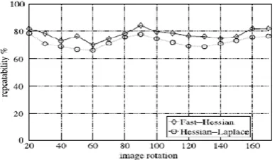
Gaussian second derivative. They are optimal for scale-space analysis Gaussians have to be decided(Fig. 2, left half), [5, 6]. This leads to a loss in repeatability under image rotations around odd multiples of . This is the weakness of Hessian-based locator. Fig. 3 shows the continuous rate of two detectors based on the image rotation using Hessian matrix. The multiples of gives the maximum continuity. This is because of the square shape of the filter. With the advantage of fast convolutions brought by the discretion, outweigh the slight decrease in acheivement. The real filters are non-ideal in many cases. Lowe uses the LoG approximations as the approximation for the Hessian matrix can be done with box filters (in the right half of Fig. 2). The integral muzzle images helps in the approximation of second order Gaussian derivatives at a very low summation cost. The calculation time therefore is independent of the filter size. As shown in Fig. 3, the performance is comparable or better than with the discretion

.

Fig. 2. Left to right: The (discretised and cropped) Gaussian second order partial derivative in y- ( ) and

xy-direction (Lxy), respectively; approximation for the

second order Gaussian partial derivative in y- (Dyy) and

xy-direction (Dxy). The grey regions are equal to zero.

Fig. 3. Top: Repeatability score for image rotation of up to . Hessian-based detectors have in general a lower

repeatability score for angles around odd multiples of . Fast-Hessian is the more accurate version of our detector

(FH-15), as explained in Section 2.3.

The box filters in Fig. 2 are Gaussian with

and denote the lowest scale (i.e. highest spatial resolution) for summation of the blob response maps.

, and are the weights applied to the

rectangular regions are kept simple for computational ability.

( )

The Hessian’s determinant is balanced by the responses of the relative weight vector w. The Gaussian kernels and the approximated Gaussian kernels helps in energy conservation,

| | | | | | | |

where | | is the Frobenius norm. The weighting changes depends on the scale for theoretical corrections. In practice, this factor is kept constant.

The normalization of filter sizes are done with respect to their size. A constant Frobenius norm for any filter size is an important aspect for the scale space analysis as explained in the next section.

The determinant of the Hessian matrix approximates the blob response in the muzzle image at location x. These responses are stored in a blob response map over different scales, and local maxima are computed as explained in Section 2.4.

2.3. Scale Space Representation

583

The use of box filters and integral muzzle images helps in the iterative filtering is not required, but instead can apply box filters of any size at exactly the same speed directly on the original muzzle image and even in parallel. Therefore, the scale space is analyzed by up-scaling the filter size rather than iteratively reducing the muzzle image size, Fig. 4. The output of the filter, introduced in previous section, is considered as the initial scale layer, to which referred as scale

(approximating Gaussian derivatives with ). The following layers are obtained by filtering the muzzle image with gradually bigger masks, taking into account the discrete nature of integral muzzle images and the specific structure of our filters.

Fig. 4. Instead of iteratively reducing the image size (left), the use of integral muzzle images allows the up-scaling of

the filter at constant cost (right).

The scale space is divided into octaves. An octave represents a series of filter response maps obtained by convolving the same input muzzle image with a filter of increasing size. An octave contains a scaling factor of 2. Each octave is subdivided into a constant number of scale levels. Due to the discrete nature of integral muzzle images, the minimum scale difference between two subsequent scales depends on the length of the positive or negative lobes of the partial second order derivative in the direction of derivation (x or y), which is set to a third of the filter size length. For the filter, this length is 3. For two successive levels, it is required to increase this size by a minimum of 2 pixels (1 pixel on every side) in order to keep the size uneven and thus ensure the presence of the central pixel. These results in a total increase of the mask size by 6 pixels (see Fig. 5). The dimensions different from , recalculates the mask introduces rounding-off errors. However, the errors are much smaller than l0 and hence this is an approximation.

Fig. 5. Filters (Top) and (Bottom) for two

successive scale levels ( and ). The length of the dark lobe can only be increased by an even number

of pixels in order to guarantee the presence of a central pixel (top).

The blob response of the muzzle image for the smallest scale can be calculated by using a filter. Then, filters with sizes , , and are applied, by which even more than a scale change of two has been received. It is a 3D non-maximum suppression which applies both spatially over the neighbouring scales. The Hessian response maps in the stack for first and last cannot contain such maxima themselves, as it is used for comparison only. Therefore, after interpolation, see Section 2.4, the smallest possible scale is correponding to a filter size , and the

highest to .

584

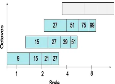
Fig. 6. Graphical representation of the filter side lengths for three different octaves. The logarithmic horizontal

axis represents the scales.

Fig.7. Histogram of the detected scales. The number of detecting interest points per octave decays quickly. The first filters within these octaves (from 9 to 15 is a change of 1.7), for large scale changes, the sampling of scales is quite high. Hence the space scale with a fine sampling of the scales is performed. This computes the integral muzzle image on the muzzle image up-scaled by a factor of 2, and hence the first octave filters with a filter of size 15. Other filter sizes used are 21, 27, 33, and 39. Then a second octave starts, again using filters which now increase their sizes by 12 pixels, after which a third and fourth octave follow. The scale change between the first two filters is only 1.4 (21/15). The lowest scale for the accurate version that can be detected through

quadratic interpolation is

The Frobenius norm always remains constant for our filters at any size, and they are already scaledormalized, and no further weighting of the filter response is required.

2.4. Interest Point Localization

A neighborhood is applied to localize interest points in the muzzle image and over the scales in non-maximum suppression. Specifically, SURF uses a fast variant introduced by Neubeck and Van Gool [8]. The maxima of the determinant of the Hessian matrix are then approximated in scale and muzzle image space with the method implemented by Brown and Lowe [9].

Scale space interpolation is important, as it is dissimilar in scale between the first layers of every octave which is relatively large.

3. INTEREST POINT DESCRIPTION AND MATCHING

SURF descriptor comprises the distribution of the intensity content within the interest point neighborhood, similar to the gradient information extracted by SIFT[7]. In SURF, the integral muzzle images help to increase the speed as the distribution of first order Haar wavelet responses in x and y direction rather than the gradient. The reduction in time for feature calculation and matching has helped to increase the strength. In SURF, new indexing step based on the sign of the Laplacian, which increases not only the strongest of the descriptor, but also the matching speed (by a factor of 2 in the best case).

The reproducible orientation fixes the interest point in the circular region. Then, a square region adjusted the selected orientation is constructed and extract the SURF descriptor from it. Finally, features are matched between two muzzle images. These three steps are explained in the following

.

3.1. Orientation Assignment

The invariant muzzle image rotation is to identify a reproducible orientation for the interest points. Computation of Haar wavelet responses in and direction within a circular neighborhood of radius

around the interest point, with the scale at which the interest point was detected. The sampling step is scale dependent and is chosen to be . The size of the wavelets are scale dependent and set to a side length of 4s. Hence use of integral muzzle images for fast filtering is done. The used filters are shown in Fig. 8. Six operations are needed to calculate the response in x or y direction at any scale.

Fig. 8. Haar wavelet filters to compute the responses in x (left) and y direction (right). The dark parts have the

weight -1 and the light parts +1.

585

maxima in vector length that are not outspoken. Both result in a misorientation of the interest point.

Fig. 9 Orientation assignment: a sliding orientation window of size detects.

3.2. Descriptor Based On Sum Of Haar Wavelet Responses

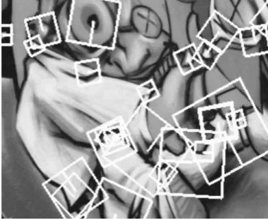
The initial step consists of the construction of a square region centered around the interest point is oriented along the orientation selected in the previous section for the extraction of the descriptor. The magnitude of this window is 20s. Examples of such square regions are shown in Fig. 10.

Fig. 10. Detail of the Graffiti scene showing the size of the oriented descriptor window at different scales. The region divide regularly into smaller square sub-regions and hence preserves important spatial information. Find Haar wavelet responses at

regularly spaced sample points for each sub-region. Let denote the Haar wavelet response in horizontal direction and the Haar wavelet response in vertical direction (filter size 2s), in Fig. 9 again. ‘‘Horizontal’’ and ‘‘vertical’’ here is defined in relation to the selected interest point orientation (see Fig. 11).1 The responses and are first weighted with a Gaussian ( ) centered at the interest point to increase the vigors towards geometric deformations and localization errors.

Fig. 10. To build the descriptor, an oriented quadratic grid with square sub-regions are laid over the interest point (left). For each square, the wavelet responses are computed from samples. For each field, we collect the sums , | |, , and | |, computed relative to the

orientation of the grid (right).

The initial set of entries in the feature vector is formed by wavelet responses and are total up over each sub-region. Extract the total of the absolute values of the responses, | | and | | to find the polarity of the intensity changes. The sub-region has a 4D descriptor vector with intensity structure

| | | | Doing this for all

regions, the results in a descriptor vector of length is 64. The wavelet responses are invariant to a bias in illumination (offset). Invariance to contrast (a scale factor) is achieved by making the descriptor into a unit vector.

Fig. 11 shows the characteristics of the descriptor for three distinctively different image-intensity patterns within a sub-region. The combinations of such local intensity patterns, resulting in a distinctive descriptor can be seen.

Fig. 11 The descriptor entries of a sub-region represent the nature of the underlying intensity pattern. Left: In case

of a homogeneous region, all values are relatively low. Middle: In presence of frequencies in x direction, the value of | |is high, but all others remain low. If the

intensity is gradually increasing in x direction, both values and | | are high.

586

SURF integrates the gradient information within a subpatch, whereas SIFT depends on the orientations of the individual gradients. This makes SURF less sensitive to noise.

The wavelet features, second order derivatives, higher-order wavelets, Principal Component Analysis, median values, average values, etc helped as SURF descriptors. The proposed sets of descriptors turned out to perform best. The sub-region, division solution helps to provide better results. The finer subdivisions appeared is considered and found to be less robust and helps to increase matching times. Obviously, the short descriptor with sub-regions (SURF-36) performs which is not as good, but allows for very fast matching .

The SURF descriptor sums a couple of similar features (SURF-128) which is also tested. It again uses the same total as before, which splits these values up further. The sums of and | | are calculated separately for and . As the sums of and

| |are split up according to the sign of , the doubling the number of features is done. The descriptor is more different and not much slower to calculate, but slower to match due to its higher dimensionality.

3.3. Fast Indexing For Matching

The symbol of the Laplacian (i.e. The trace of the Hessian matrix) for the underlying interest point is included, for fast indexing during the matching stage. The interest points are found at blob-type structures basically. The symbol of the Laplacian differentiates bright blobs on dark backgrounds from the reverse situation. This feature can be done without extra computational cost since it was already computed during the detection phase. In the matching stage, only compare features if they have the same type of contrast, see Fig. 12. Hence, this minimal information helps in faster matching, without reducing the descriptor’s performance. This is also of advantage for more advanced indexing methods.

Fig. 12 If the contrast between two interest points is different (dark on light background vs. light on dark background), the candidate is not considered a valuable

match.

4. THE PROPOSED CATTLE IDENTIFICATION APPROACH

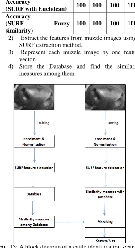
The proposed approach for the identification , as illustrated in Fig. (13), mainly consists of two phases: Training and Testing. The algorithm is detailed below as block diagram.

Training phase

1) Collect and normalize all training muzzle print images.

2) Extract the features from muzzle images using a SURF extraction method.

3) Represent each muzzle image by one feature vector.

4) Store the Database and find the similarity measures among them.

Fig. 13: A block diagram of a cattle identification system using muzzle print images.

Testing phase

1. Collect and normalize the testing muzzle print image.

2. Extract the features of the collected image using SURF.

3. Compare the similarity measure of feature vector with database feature vectors.

4. Matching to find muzzle or not and position as a max similarity value if muzzle.

5. RESULT AND DISCUSSION

In our work, normalized muzzle images are used. Using Speeded up Robust Feature method, the descriptors are calculated for each image. These features are fuzzified using Gaussian function and similarity values of each image with other images are calculated and saved in the database. When an input image enters the system, its SURF features are calculated, fuzzified using Gaussian function and similarity values of each image with that in the database are calculated. The similarity value is compared with all values in the database. If maximum of

Number of Images 10 20 30 40

Accuracy

(SURF with Euclidean) 100 100 100 100 Accuracy

(SURF Fuzzy

similarity)

587

this similarity measure value is greater than second largest unique similarity value in the database, it is a recognized muzzle image in database, with position at highest similarity value. Otherwise it is a new muzzle image.

Here total 43 images of 43 different cows are there in the database. Algorithm is tested for 10, 20, 30 & 40 images with others as unknown. The accuracy value (%) is calculated using the equation 10 and results shown in table below.

Here we can see that SURF with fuzzy similarity gives the same results as with Euclidean distance. Here the proposed method works well with small amount of added impulse noise also.

6. CONCLUSION

The new application of the beef cattle identification using muzzle pattern based on SURF Fuzzy similarity approach has been proposed. The performance of the proposed identification mechanism is similar to the existing method like SURF Euclidean and significantly better than the previous methods, i.e, the identification method proposed by Barry et al. The average accuracy of PCA with Euclidean is 52%, PCA with fuzzy similarity is 95% and with Fuzzy SURF is 100%. Fuzzy SURF is also rotation and scale invariant. Small noise resistivity(<10%) is there

in proposed similarity method compared with Euclidean method.

REFERENCES

[1] P.A. Viola, M.J. Jones, “Rapid object detection using a boosted cascade of simple features”, in: CVPR, issue 1, 2001, pp. 511–518.

[2] P. Simard, L. Bottou, P. Haffner, Y. Le Cun, “Box lets: a fast convolution algorithm for signal processing and neural networks”, in: NIPS, 1998.

[3] K. Mikolajczyk, C. Schmid, “Indexing based on scale invariant interest points, in: ICCV”, vol. 1, 2001, pp. 525–531.

[4] T. Lindeberg, “Feature detection with automatic scale selection”, IJCV 30 (2) (1998) 79–116.

[5] J. J. Koenderink, “The structure of images”, Biological Cybernetics 50 (1984) 363–370.

[6] T. Lindeberg, “Scale-space for discrete signals”, PAMI 12 (3) (1990) 234–254.

[7] D. Lowe, “Distinctive image features from scale-invariant keypoints”, IJCV 60 (2) (2004), 91–110. [8] A. Neubeck, L. Van Gool, “Efficient non-maximum suppression”, in: ICPR, 2006.