DOI: http://dx.doi.org/10.26483/ijarcs.v9i2.5897
Volume 9, No. 2, March-April 2018
International Journal of Advanced Research in Computer Science
RESEARCH PAPER
Available Online at www.ijarcs.info
ISSN No. 0976-5697
EFFECT OF TEXTURE FEATURE COMBINATION ON SATELLITE IMAGE
CLASSIFICATION
Dr. Mohammed Sahib Mahdi Altaei Department of Computer, Collage of Science
Al-Nahrain University Baghdad, Iraq
Saif Mohammed Ahmed
Department of Computer, Collage of Science Al-Nahrain University
Baghdad, Iraq
Dr. Hayder Ayad
Department of Computer, Collage of Science Baghdad University
Baghdad Iraq
Abstract: This paper presents a method for SIC to classify a PatternNet satellite image dataset taken from Google Earth and Google Map
Application newly adopted in 2017, this SIC method use firstly a pre-processing step to verify the way of how represent the gray level of each sample image using multiple features based descriptors to handling the problem of selecting the descriptors for SIC. It suggested to use several type of texture feature extraction method, each of these method tested with the Support Vector Machine (SVM) to verify its ability to extract d a discriminative features. Also the feature selection method used to remove the less informative features of each method to get the more relevant features, finally the decision result of each feature extraction method from the classifier tested with feature combination methods, it is used to improve the final decision of the SIC method by combine multi feature extraction method.
Keywords: Texture Features, Remote Sensing, Features Combination, Satellite Image Classification, Edge Histogram Descriptor, Local Binary
Pattern, Grey Level Co-occurrence Matrix, Support Vector Machine
I. INTRODUCTION
Remote Sensing (RS) is the art of science that acquiring information about a specific area, object, or phenomena by analysing the obtaining data from the device that is not contact with the area, object or phenomenon. The human eye is like a sensor that responds to the reflected light from an object, and pictures the object according to received light intensities [1]. RS in the classical sense is not a scientific discipline; it is rather a big variety of diagnostic methods by using electromagnetic waves. In some cases where electromagnetic methods fail, then sound waves or other elastic waves are used. It is obvious that RS required in many different techniques and skills. The applications cover a wide range of humanities disciplines, e.g. Botany, archaeology, geology, meteorology and security aspects, etc. [2].
There are several methods and techniques that are used in RS images, the choice of classification method depend on many regards such as: information gathered from different sensor, the sample label is known or not, the training sample nature used in RS image classification, the pixel informative nature of the data, the number of the output for each spatial data element, etc. [3]. Different methods and algorithms are used for RS image classification such as maximum likelihood, minimum distance, Artificial Neural Network (ANN), decision tree, linear discriminant analysis, Support Vector Machine (SVM), whilst the search on the optimal one is still continue in terms of suitability for different applications [4], The feature Selection method used to minimize the number of features [5].
II. LITRETURE REVIEW
There are a great deal of focus was granted to satellite image classification. Numerous methods were developed for achieving more efficient techniques that serving the applications in the field of interest. The most significant literatures are mentioned with details in the following:
Thirteen different descriptors based on color, texture and the structure were used to extract the image features from Very High Resolution (VHR) satellite image retrieved from Google Earth Application, there is a nineteen class of the Airport, beach, bridge, football field, river, etc. This dataset contains fifty samples for each class, which is used for training and testing the classifier. The thirteen feature extraction methods are Scale-Invariant Feature Transform (SIFT), Geometric Blur (GB), GIST, Self-Similarity (SSIM), Local Binary Pattern (LBP), Maximum Response (MR) filter bank, Leung-Malik (LM) filter bank, Gabor filter bank, Color Histogram (Colorhist), Hue, Opponent (OPP) and Color Pool, The Support Vector Machine (SVM) and K- Nearest Neighbor (KNN) classifiers used for classification step. Each of these feature methods is fed to the classifier lonely, and then all features are combined to get the cooperation score of them. The result shows that the more accuracy result was achieved when using the SIFT feature extraction method with the SVM classifier in comparison with the use of KNN classifier [6].
feature method based on pixel oriented and region oriented methods, then the fusion system is used to make a decision based on just good features. The test includes data segmentation, features extraction, and then SVM based classification. The classification result showed reliable classification for multispectral data [7].
The ANN is used to classify satellite images given by LandSat-8. The image is first encoded by divided it into equal size of blocks, then these blocks are quantized for estimating the code of each block. The features of each block are extracted depending on the probability of that block. These features are then used to train the ANN, which prepare to use a newest image sample in the ANN classification that indicates the validation of the ANN classifier [8].
The SVM Classifier has been proposed to classify a very high resolution satellite image collected from google map application and google earth imagery, several number of classes have been used, several features extraction methods used to extract features from each sample per class, the features are then entered into a Scatter analysis method to select the most informative features that increase the classification result. The feature extraction method that have been used are special technique like Speeded Up Robust Features and also the texture extraction features have been used like the Grey Level Co-occurrence Matrix and Local Binary Pattern. After get the probability result from each of the feature extraction method separately the feature combination method used to improve the final decision of the method, the result show that the texture features work very good than the Special technique [9].
III. PROPOSED SATELLITE IMAGE CLASSIFICATION
The Proposed Satellite Image Classification (SIC) include four major steps, pre-processing step includes loading several samples of images from specific class that randomly chosen from the used satellite images dataset The conversion from RGB color band into grey scaled image is then applied. Three feature extraction methods are adopted, they are: LBP based on Rotated (RLBP) with different radius, Gray Level Co-occurrence Matrix (GLCM) that applied on grey and RGB bands that used with different block size and Edge Histogram Descriptors (EHD). There methods are employed once individually and then combind with each other, in another time to test its effect on the classification performance. The classification decision based on descriptors combination is stored in a comparable features vector in the database. Then, scatter analysis as a feature selection method is used to test feature vector and remove the unusable descriptors from the database. The SVM classifier is employed to decide the classification of each image sample in terms of the comparison between the features vector of test image sample and those found in the database. Finally the features combination method applied to combine the classification result from each feature extraction method to improve the classification result. As shown in Figure (1):
Fig.1: The Proposed Satellite Image Classification Method
A. Pre-Processing Step
The process of converting the RGB color image to grayscale image is the first of pre-processing step. There are two methods work for the conversion have been proposed each of which has the advantage and disadvantage when it is working with a different feature extraction method that require the gray image as shown in Equations 1 and 2.
Gr= (0.299 × R) + (0.587 × G) + (0.114 × B) (1)
Gr= (Rn + Gn + Bn + UV)/4 (2)
Where, Rn= ((R × 0.299) + (R × 0.587) + (R × 0.114)) / 3
Gn= ((G × 0.299) + (G × 0.587) + (G × 0.114)) / 3
Bn= ((B × 0.299) + (B × 0.587) + (B × 0.114)) / 3
The UV can be calculated by the intensity band (Y) as follows:
The second pre-processing step is the image enhancement that concerned with increase the contrast of the image by applying a linear fitting model on each pixel in the image to be transformed from the attended scale to the full contrast situation where the pixel values become actually in between 0-255 as shown in Equation (3).
a= 255/ (Max-Min) b=(255×Min)/(Max-Min)
Gg=a × GI(x, y) + b (3)
Where Max is the max gray pixel value, Min is the min gray pixel value, GI is the gray image pixel value, Gg represent the enhanced gray image. B. Feature Extraction Step
Texture features are a type of low level feature, they are
not common as color feature, but it used in many application of pattern recognition field and gives good information especially in image classification systems. Such features describe the content of real world images includes trees, clouds, airplanes, and other. Three types of texture features used are GLCM, EHD and RLBP. The GLCM is firstly quantizing the image into few grey levels, which leads to remove the possible noisy pixels may found in the sample image. Such that, there most dominant color is found in the quantized image that can be used to represent the objects clearly. This requires partitioning the image into a number of blocks with predetermined size. The frequency of each quantized image block is help to compute the probability of appearance each pixel in that block, then these probabilities are substituted in Equations (4-16) to compute the meant textural features of current image block by GLCM. To achieve more description, the computational processes are considered in the four orientations 0o, 45o, 90o, and 135o. Therefore, there are 13 descriptive features are resulted for each image block. … (4)… (5)
… (6)
Where ω is the angular second moment, Pij is the is the Co-occurrence value at position i and j, C is the contrast, µi and µj, σi and σj are the means and standard deviation of the rows and columns respectively. … (7)
Where σ2 is the variance, µ is the mean of both µ i and µj. … (8)
… (9)
Where is the inverse difference moment, α is the sum of average, Pi; x+yis the probability of the co-occurrence matrix which in the coordinates x and y are summing. … (10)
… (11)
… (12)
… (13)
… (14)
… (15)
… (16)
Where, Sv is the sum variance, Se is the sum entropy, E is
the entropy, Dv is the difference variance that same as the
variance of Px-y, De is the difference entropy, and, A and B are
the information measures of the correlation.
Where, HX and HY are entropies of Pxand Py, which are
given as follows:
[image:3.595.310.542.272.393.2]
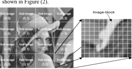
EHD concerned with computing the texture features, it is used to extract texture features that forming edges of the object shape in the image sample. Filter technique is used to extract the most dominant edge in an image block. So, EHD is applied on the gray image, and then partition the image into 16 equal blocks. For each block, the five edge filters of the EHD are computed in terms of sub block of 2×2 size as shown in Figure (2).
Fig.2 Image partitioning into sub blocks in EHD
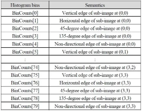
[image:3.595.308.555.497.551.2]Therefore, each sub block is represented by five numbers are the computed edge values of 2×2 sub block in the five directions: 0o, 90o, 45o, 135o, and non-directional edges as shown in Figure (3).
Fig 3: EHD filters, (a) Vertical filter, (b) Horizontal filter, (c) 45 degree filter, (d) 135 degree filter, (e) non-directional filter.
Table 1: Summary of the 80 histograms bins of EHD .
RLBP is adopted to record the relation between a central pixel and its circular neighbors. The main difference between the Block LBP and RLBP is that the first is static block size, while the latter is more dynamic computing in which the result can be obtained with different radii that prepare to deal with many neighbors. The process is start by determining the number of neighbors and the radius of neighborhood. The RLBP is applied on gray image, in which the position of the circular pixel is determined by Equations (18 and 19), whereas the maximum number of the neighbors that determined using Equation (20).RLBP is used to implements the comparison between the central pixel and its neighbors that applied in the same manner of the Block Local Binary Pattern with Equation (20). The obtained histogram of new LBP pixel value is representing the feature vector of current pixel.
Ip= I (xp, yp) … (17)
xp = xc + R Cos ( 2πp / N) … (18) yp = yc – R Sin ( 2πp / N) … (19)
Where I(xp, yp) represent pixel neighbor; in which p= 0, 1,
2,…..,N .
DD= max |Ip – Ic| … (20)
Where, DD is the maximum neighbor N is the number of neighbors, Ic is one of the neighbor pixels for p=0, 1, 2… N,
and Ic is the center pixel.
The determination of the DD and the maximum value of the neighbors around each of the pixel according to the number of neighbors and the length of the radius, the same way is used to find the threshold value of the LBP is also used to determine the RLBP threshold, the difference is the length of the radius that should be taken into account. Therefore, the computation starts from the DD pixel value and continue to the pixels in the circle around the center pixel.
C. Feature Selection Step
Feature selection methods is important in any classification methodology, these method try to select most relevant and effective features from a set of extracted features and remove as possible the not efficient features. Several method adopt for this work, in proposed SIC method the Scatter analysis approach has been used as a feature selection method. The proposed SIC method makes the use of inter scatter since it
will detect the features that can change the right decision of the classifier, the idea is that to after calculate each V vector from and feature extraction method, this vector used as input to the scatter analysis method and calculate the inter scatter Ia
to the vector through the Equation (21). After that, the result of inter scatter calculation will be sorted and then analysis to detect ineffective features, the highest value of the inter scatter analysis will be removed because it causes distortion to the accuracy result.
… (21)
Where in intra scatter equation, i is the number of class, j is the number of the features. In the inter scatter equation, N is the number of classes, the σi;j is the standard deviation of the ith class with the jthfeatures that belong to it, the μ
i;jis the
mean of the ith class with the jthfeatures that belong to it.
D. Classification Step
There are several types of conditions must be considered to select the classifier in SIC systems, they are: classification per pixel or subpixel, the fusion is for multi sensor or multi resolution, the type of data to be classified, spectral resolution, spatial resolution, and others. The most recent common classifiers used in satellite image classification are: Support Vector Machine (SVM), Artificial Neural Network (ANN), Maximum Likelihood (MML), Fuzzy set classifiers, and decision tree classifier. Each of these methods has advantage and disadvantage with its usage.
SVM is one type of machine learning algorithm, it is a supervised classification method proposed to solve the binary classification (two classes only) problem, but later the SVM developed to be used in multiclass classification. In the multiclass classification, there two ways are used to classify data either in one versus the rest class or pair wise classifier. In the first approach the sample in each class is assigned to the one of classes with higher probability, while in the second approach the comparison are made between every two classes and the sample are assigned to the higher votes of each class have been used.
E. Features Combination
step with the mean rule, the only difference is that instead to take the mean of the probability take the product of the probability output from different feature methods.
IV. RESULTS AND DISCUSSIONS
The development of the satellite imagery has been led to an easy way to get useful information from land cover, this information can be used in many projects like Security, Geology, Military operations, Meteorological and others. As a result the behavioral performance examined through data analysis of the satellite imagery by using training and testing steps for the classification system. In the present work, the preprocessing step used to convert the input images to gray levels depend on the type of feature extracted method, several feature extraction methods used to describe the information from different classes of satellite imagery, these features extracted from all satellite imagery, then these features has been entered in to feature selection method in order to remove as possible the not useful features, then the selected features divided in to part used to train the classifier and the other part used to test the performance of these extracted features. The post processing step include take the result from the classifier from each feature extraction methods, analysis their performance then used them to for combination method to improve the classification result. In the next paragraphes the detailed explanation of each of the previous steps discussed, and the results are presented in tables and figures, then qualitative and quantitative of the proposed satellite images classification method evaluated. The implementation of the proposed methods was done using C# programming language, which is executed under windows 10 operating system of 64 bit type.
A. Remote Sensing Dataset
There are several Benchmarks dataset proposed to evaluate the performance of many satellite image applications, these datasets used to verify how the systems built in an effective and efficient way. Some of these datasets are UC Merced, WHU-RS19, RSSCN7, Aerial image and NWPU-RESIC45. Each of the benchmarks dataset has several challenges must be taken into the consideration when choose the steps to build the application, some of these challenges are they are land use/ land cover images, spatial resolution , spectral resolution, the number of classes in each data sets and also the number of samples per class, and others. All of these must take when selecting the feature extraction methods, and also the classifier used in the classification system and many other steps in the system [10]. There are different dataset that can be used in different application and used to evaluate the proposed work [11]. In this proposed SIC method PatternNet Dataset used.
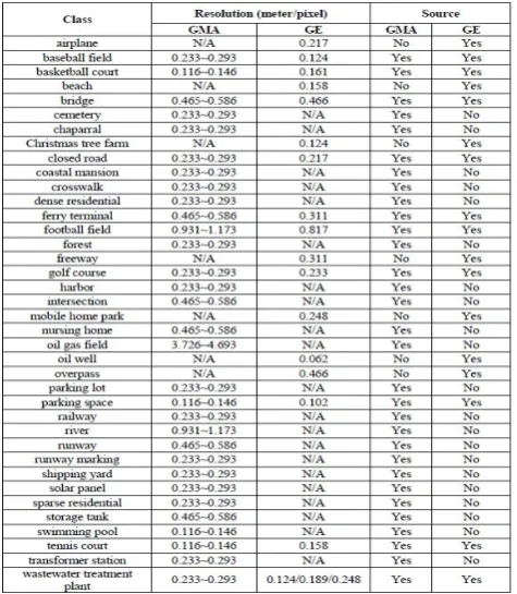
[image:5.595.310.548.78.351.2]PatternNet dataset have been proposed recently in 2017, it consists of a large number of high resolution remote sensing images that collected for RSIR research. These images are collected from Google Maps API (GMA) and Google Earth Imagery (GEI) for United States (US) cities. It contains 38 classes such as Airplane, Baseball field, Beach, Football field, Intersection, Oil gas field, Swimming pool, and others. Each of these classes contains an 800 sample per class. The sample image resolution is 256×256 pixel, the spatial resolution of the dataset samples is varying from one to other, in which the lower value is about 0.062m while the highest one is about 4.693m, Table (2) shows numerical description for the spatial resolution of the PatternNet dataset.
Table 2: Spatial resolution of PatternNet dataset given by GMA and GEI..
This dataset have different varies with spectral and spatial resolutions; also the objects in each sample may have different scale, rotation, illumination, and other situations, which could pose real challenges for the used classification method to be distinguished between such situations. Thus, the used classification method and the choice of employed descriptors should be chosen carefully. The first 30 classes of the PatternNet dataset with 40 samples per class have been adopted for testing the performance of the proposed method, in which 20 samples are used for the training the SVM classifier, and another 20 samples are used for testing and evaluating the proposed method.
B. Pre-Processing Results
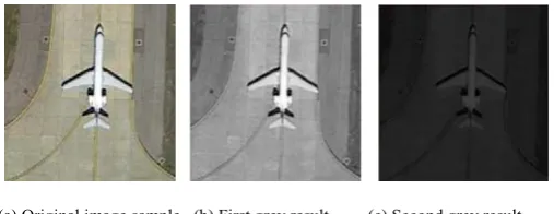
The preprocessing step adopt firstly to the sample image in order to convert the input sample image from RGB color space (24 bit) to gray scale image (8 bit), this conversion will be better to the analysis for machine learning, also to decrease the time of computation and effect to the final result of the accuracy of the classification. Two algorithms have been used in this step each of which tested with feature extraction method to verify their ability to extract useful descriptors with the gray image. The Equation (1) which is take the weighted of the three color space (RGB), this algorithm show that most luminance result due to the weighted percentage of the taken input wavelength as shown in figure (4.b) .
(a) Original image sample (b) First grey result (c) Second grey result
Fig (4): Results of the two adopted grey conversion methods.
(a) Enhanced first grey result. (b) Enhanced second grey result.
Fig (5): Results of contrast enhancement applied on grey conversion methods shown in Figure (4).
C. Feature Extraction Result
Feature extraction is an important stage due to it prepares to analyze the image information and enable to get useful features that processed as descriptors in the classification stage. This stage deals with several types of descriptors to extract effective features from the dataset. The results of the employed texture features.
GLCM Results
GLCM is applied on the four image bands, the best max quantize level value has been chosen to be 80. Each quantized pixel is interconnected with its four neighbors that ling along the extensions of the four considered orientations 0o, 45o, 90o, and 135o, this is carried out through five considered values of the distance between the quantized pixel and its neighbors, they are: 1, 2, 3, 4, and 5 pixels. The resulted normalize values of the extracted 13 GLCM features of the used four color bands R G B and Grey and for two distance between the center pixel and its neighbors, so there will be 104 features as result from each sample image.
EHD Results
The application of EHD used to extract edge texture features, this leads to obtain a behavioral histogram of 80 bins length from the image sample. This histogram describes the detected edge in an image sample according to a specific threshold. The normalized features vector of the EHD histogram of the used Grey band at threshold value is 12 used in the proposed SIC method.
RLBP Results
RLBP take the consideration of rotation invariant to improve the classification result, as discuss before the idea is to take the max value of the neighbors and start all of the weighted neighbors from this value, different radius has been tested with eight neighbors in order to select the best circular.
Table (3) show that eight neighbors with multi radius classification accuracy result.
Run No. of Features
No. of Neighbors
Radius Accuracy %
1 256 8 1 86.66 2 256 8 2 84.33 3 256 8 3 88.16 4 256 8 4 86.5 5 256 8 5 80.6 6 256 8 6 79.16 7 256 8 7 73.33
D. Feature Selection Results
Scatter analysis method adopts to implement the feature selection function. The use of this method is due to it is an efficient and operated during little time of comparisons between contributed features. The scatter analysis is depends on finding inter (between classes) and intra (with in same class) classes to point out the features that make possible confliction in the classification decision. Therefore, the inter scatter is used to find out the features that may change the right decision of the classifier. So, the extracted features vector V is input to scatter analysis for calculating the inter scatter by Equation (21). The resulted inter scatter is analyzed to detect ineffective features, the ineffective features are those possess highest value of the inter scatter, which candidate to be removed due to some distortion that happen by such features. The features that pointed as useable and can be effectively contributed in the process of classification decision making are stored in list of useable features called Pass Features List.
1. GLCM Features Selection Results
GLCM features are first analyzed with different values of quantization levels (QL) applied on the four adopted color
bands R, G, B, and Gr. The number of features that have been
extracted from each band is 13 features. Whereas, number of obtained features becomes 52 features when they extracted from the four color bands. It is noticeable that the highest classification score is achieved whenever the number of quantization levels is 80.Latter, GLCM features are analyzed with different values of coverage distance, which can take one of the following values: 1, 2, 3, 4, and 5 pixels. The average classification scores for different distances between the central pixel and its neighbors when applied on the four adopted color bands at number of quantization levels is fixed on 80 levels. It is noticeable that the highest classification result is achieved at the case when two distances are used together at eighth run, where these distances are: 1 and 4 pixels so as a result there will be 104 features extracted from each sample image. In addition, best discriminative indication for the chosen two distances is found when the 80 quantization levels are applied on the adopted four color bands (R, G, B, and Gr). This yields
[image:6.595.37.291.52.150.2] [image:6.595.313.552.67.195.2] [image:6.595.47.263.175.279.2]Table (4) Scatter analysis of SVM classifier based on GLCM features.
Run No. of Features
Removed Features
Current No. of Features
Accuracy %
1 104 4 100 83.5
2 104 8 96 84.5
3 104 12 92 84.5
4 104 16 88 84.5 5 104 20 84 84.66 6 104 24 80 84.5 7 104 28 76 85.166 8 104 32 72 85.833 9 104 36 68 86.333 10 104 40 64 84.33 11 104 44 60 84.66 12 104 48 56 85.66
2. EHD Features Selection Results
Several threshold values are tested to choose the best one that gives best classification score, in which the used threshold values are ranged in between (5-15). Table (5) presents the average SVM classifier accuracy of the used 80 EHD features with different edge threshold values applied on 20 samples of airplane image. It is shown that the threshold value of 12 gave best classification results in comparison with other values. Thus, the threshold value is determined to be 12 in the following processing.
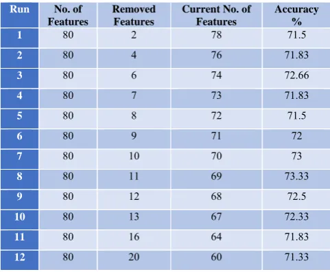
Table (6) presents the average classification scores of several SVM classifier tests based on EHD features, in which the 80 extracted features per sample are analyzed by the scatter analysis to select the most discriminative features that shows best classification result. The highest classification score is achieved at the eighth run when the classification depends on a number of contributed features is 69 features. It is noticeable that the classification score increases with discarding the weak feature at each run time till reaching the best score of about 72.66% at the eighth run, and then this score decreases with increasing the number of discarding features. This indicates that the coalition work of the EHD features becomes optimal when the contributed features are just 69 features.
Table (5) SVM classification score using EHD features at various threshold values.
Run Threshold value SVM Accuracy %
1 5 69.5
2 6 69.166
3 7 70.83
4 8 71
5 9 72.166 6 10 71.66 7 11 71.833 8 12 72.66
9 13 71.5
10 14 71.66 11 15 71.66
Table (6) Classification scores versus number of EHD features.
Run No. of Features
Removed Features
Current No. of Features
Accuracy %
1 80 2 78 71.5
2 80 4 76 71.83
3 80 6 74 72.66
4 80 7 73 71.83 5 80 8 72 71.5
6 80 9 71 72
7 80 10 70 73
8 80 11 69 73.33 9 80 12 68 72.5 10 80 13 67 72.33 11 80 16 64 71.83 12 80 20 60 71.33
3. RLBP Features Selection Results
The radius of circular neighboring area is tries to be optimized with different values. Table (7) presents the classification scores of eight neighbor pixels with different considered values of the radius. It is noticeable that the classification accuracy of different runs at which the radius of circular coverage area is varies from 1-7 are found differs according to the radius value. The radius of 3 pixels value gives the best classification result in comparison with others. Also, it is shown that the classification accuracy is increased with increasing the radius value till reaching the optimal one when the radius is 3 pixels that gives classification score of about 88.16%. Then this score decays slowly with increasing the radius value. The reason behind such behavior is due to the increase of radius causes to include more useful information inside the considered area that leads to increase the classification score. While, the decrease of the classification is because the more included neighbors cause to include additional non-homogenate neighbors that leads to confuse the classification results.
Table (7) RLPB classification of 8 neighbors and different radii of considered coverage area.
Run No. of Features
No. of Neighbors
Radius Accuracy %
1 256 8 1 86.66 2 256 8 2 87.33 3 256 8 3 88.16 4 256 8 4 85.5 5 256 8 5 82.6 6 256 8 6 79.16 7 256 8 7 73.33
[image:7.595.312.553.79.277.2] [image:7.595.37.287.86.281.2] [image:7.595.36.284.600.779.2]256 features are used to be contributed in the classification decision.
Table (8) RLBP classification scores versus used features.
Run No. of Features
Removed Features
Current No. of Features
Accuracy %
1 256 0 256 88.16
2 256 5 251 84
3 256 10 246 83.5 4 256 15 241 83.66 5 256 20 236 84.83 6 256 25 231 84.16 7 256 30 226 83.5
8 256 35 221 83.83
9 256 40 216 82.33
10 256 45 211 82.66
E. Classification Results
The results of classification stage are already adopted after determining the descriptors that contributed in the classification process by means the scatter analysis. This refers to collect enough information about each class through the training stage. Supervised SVM classifier is used to classify the contents of satellite image that want to be classified. The classification tests are carried out by using SVM classifier using the remaining 20 samples of the 30 classes. Each of the three methods (GLCM, EHD, RLBP) has been tested randomly over 10 random run, this randomize of the training and testing samples is to show how each method work even with generalization of the samples.
The average of the 10 random runs with GLCM show that the score of the classification accuracy is about 90.514%, in which the Standard deviation of these 10 random runs is about ±0.8.
The average of the 10 random runs with EHD show that the score of the classification accuracy is about 80.296%, in which the Standard deviation of these 10 random runs is about ±1.040.
The average of the 10 random runs with RLBP show that the score of the classification accuracy is about 93.883%, in which the Standard deviation of these 10 random runs is about ±0.930.
F. Features Combination Results
In the proposed SIC method, two kinds of the classification accuracy approaches have been adopted, first a single classifier and second the combine of multiple classifiers result. All the experiment results of the previous sections show that a single classifier result which means that the classification accuracy take with separate feature extraction method according to its feature vector. Mainly the previous method show that classes can have more than one template to represent them, so that in order to increase the information of each sample and make the final classification decision depend on multiple feature vector to improve the categorization problem and the final accuracy result.
In the proposed SIC method, the post processing of feature combination is applied by use two types of the fusion system which are the mean and product rule, both of these rule applied to get the experiment performance of the final
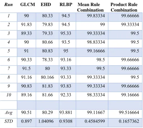
decision, these two types are both kind of ensemble approach. After testing using different features vector output from the three methods, the best classification decision founded when the combination between the classifier output of three feature extraction methods which are GLCM, RLBP and EHD, Table (9) show the combination results with mean and product rule methods.
Table (9) Results of individual classifier and combination of multiple classifiers.
Run GLCM EHD RLBP Mean Rule Combination
Product Rule Combination
1 90 80.33 94.5 99.83334 99.66666
2 91.83 79.83 94.5 99 99.33334
3 89.33 79.33 95.33 99.33334 99.5
4 90 80.66 93.5 98.83334 99.5
5 91 80.83 95 99.16666 99.5
6 90.33 78.33 93.16 98.5 99.66666
7 91.5 80 93.33 99.5 99.66666
8 91.16 80.166 93.33 99.33334 99.5
9 90.83 81.83 93.83 99.33334 99.66666
10 89.16 81.66 92.33 98.33334 99.16666
Avg 90.51 80.29 93.881 99.11667 99.516664
STD 0.897 1.04096 0.9308 0.4584599 0.1657362
V. CONCLUSION
By interpretation the results of from the combination of the three feature extraction methods, the results show that the combination of multiple classifier is better than the output from single classifier. On the other hand the comparison between the two combinations of the fusion methods with their classification accuracy, the product rule show that better result with accuracy 99.516664% and Standard deviation 0.1657362. also the converting of sample image from color to grayscale effect directly the classification accuracy result, The feature selection method work good into select the most informative descriptors from different feature extraction method, as a result it make the classification accuracy result better.
VI. ACKNOWLEDGMENT
I special thanks to my supervisor Prof. Dr. Mohammed S. Altaei who gave me all the supporting, helpfulness, assistance, encouragement, valuable advice, for giving me the major steps to go on to explore the subject, sharing with me the ideas. Grateful Thanks are due to the Head of Computer Science Department, and the staff of the Department at College of Sciences of Al-Nahrain University for their kind attention.
VII. REFERENCES
[1] Lillesand, T. M, Kiefer, R.W and Chipman, J.W, “Remote Sensing and Image Interpretation,” Fifth Edition, John Wiley & Sons, 2003.
[2] Matzler, C, “Physical Principles of Remote Sensing,”
University of Bern, Switzerland, 2008.
[image:8.595.35.290.102.272.2] [image:8.595.313.554.165.379.2]techniques,” International Conference on Control, Instrumentation, Communication and Computational Technologies (ICCICCT), Kanyakumari, Pages 554-557, 2014.
[4] D. Lu and Q. Weng, “A survey of image classification
methods and Techniques for improving classification performance,” International Journal of Remote Sensing, Vol. 28, No. 5, PP. 823-870, 2007.
[5] Shahweli, Z. and B. Dhannoon, "NEURAL NETWORK WITH NEW RELIEF FEATURE SELECTION FOR PREDICTING BREAST CANCER BASED ON TP53 MUTATION." International Research Journal of Computer, Vol.4, No. 12, 2017.
[6] Lijun Chen, Wen Yang, Kan Xu and Tao Xu, “Evaluation
of local features for scene classification using VHR satellite images,” Urban Remote Sensing Event (JURSE), IEEE, PP. 385-388, 2011.
[7] Hela Elmannai, Mohamed Anis Loghmari and Mohamed Saber Naceur,“Support vector machines for remote-sensing image classification,” Image and Signal
Processing for Remote Sensing VI, International Society for Optics and Photonic, Vol. 2, PP. 68-72, 2013.
[8] Altaei, M. S. M. and A. D. Mhaimeed, “Satellite Image
Classification Using Image Encoding and Artificial Neural Network,” International Research Journal of Advanced Engineering and Science, Vol. 3, No. 2, PP 149-154, 2017.
[9] Altaei, M. S. M and Saif Mohammed A., “Satellite Image Classification using Multi Features Based Descriptors,” International Research Journal of Advanced Engineering and Science, Vol. 2, No. 4, PP 87-94, 2018.
[10] W. Zhou, S. Newsam, C. Li, and Z. Shao, “PatternNet: A
benchmark dataset for performance evaluation of remote sensing image retrieval,” arXiv preprint arXiv:1706.03424, 2017.