Laboratory of Phonetics and Speech Technology Institute of Cybernetics at Tallinn University of Technology
Estonia
tanel.alumae@phon.ioc.ee
Abstract
This paper compares two approaches to lexical compound word reconstruction from a speech recognizer output where compound words are decomposed. The first method has been proposed earlier and uses a dedicated language model that models compound tails in the context of the preceding words and compound heads only in the context of the tail. A novel ap-proach models imaginable compound par-ticle connectors as hidden events and pre-dicts such events using a simple N-gram language model. Experiments on two Estonian speech recognition tasks show that the second approach performs consis-tently better and achieves high accuracy.
1 Introduction
In many languages, compound words can be formed by concatenating two or more word-like particles. In Estonian (but also in other languages, such as Ger-man), compound words occur abundantly and can even be built spontaneously. In a corpus of written Estonian consisting of roughly 70 million words, the number of different word types (including inflected words forms) is around 1.7 million and among those, around 1.1 million (68%) are compound words.
In large vocabulary continuous speech recogni-tion (LVCSR) systems, an N-gram statistical lan-guage model is used to estimate prior word prob-abilities in various contexts. The language model vocabulary specifies which words are known to the system and therefore can be recognized. However,
the large amount and spontaneous nature of com-pound words makes it difficult to design a language model that has a good coverage of the language. In addition, when vocabulary is increased, it becomes more difficult to robustly estimate language model probabilities for all words in different contexts. In order to decrease the lexical variety and the resulting out-of-vocabulary (OOV) rate, compound words can be split into separate particles and modeled as sepa-rate language modeling units. As a result however, the output of the recognizer consists of a stream of non-compound units that must later be reassembled into compound words where necessary.
The paper is organized as follows. In section 2 we describe the approach to statistical large vocabulary language modeling for Estonian. Section 3 describes the two approaches for compound word reconstruc-tion in more detail. Results of a variety of exper-iments are reported in section 4. Some interesting error patterns are identified and analyzed. We end with a conclusion and some suggestions for future work.
2 Language modelling for Estonian
Estonian is an agglutinative and highly inflective language. One or many suffixes can be appended to verb and noun stems, depending on their syntactic and semantic role in the sentence.
Estonian is also a so-called compounding lan-guage, i.e. compound words can be formed from shorter particles to express complex concepts as sin-gle words. For example, the wordsrahva‘folk’ and
muusika ‘music’ can be combined to form a word
rahvamuusika ‘folk music’ and this in turn can be combined with the word ansambelto form rahva-muusikaansambel‘folk music group’.
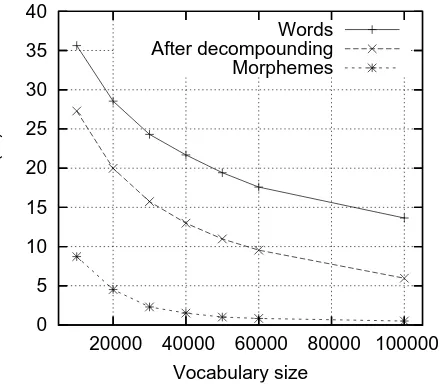
As a result, the lexical variety of Estonian is very high and it is not possible to achieve a good vocab-ulary coverage when using words as basic units for language modelling. Figure 1 compares the out-of-vocabulary (OOV) rates of three different vocabu-laries: words, words after decompounding, and after full morphological decomposition. The vocabular-ies are selected from a corpus described in section 4.1 and the OOV-rates are measured against a set of sentence transcripts used for speech recognition. The OOV-rate was measured using varying vocabu-lary sizes.
It is clear from the experiments that neither words nor decompounded words are suitable for language modelling using a conventionally sized vocabulary. The OOV-rate of the word-based vocabularies is much over what can be tolerated even when using a very large 800K size vocabulary. It can be seen that after splitting the compound words, the OOV-rate is roughly halved. Still, even when using a large 100K vocabulary, the OOV-rate is about 6% – too much to be used in large vocabulary speech recog-nition. However, the OOV-rates of morphemes is much lower and can be compared with the
0 5 10 15 20 25 30 35 40
20000 40000 60000 80000 100000
OOV(%)
[image:2.595.302.522.102.295.2]Vocabulary size Words After decompounding Morphemes
Figure 1: Out-of-vocabulary rate of different vocab-ularies.
rates of English word-based vocabularies of similar sizes. The OOV-rate of the morpheme-based vocab-ulary reaches the 2% threshold already when using a 40K vocabulary.
When using morphemes as basic units for lan-guage modelling, the output of the decoder is a se-quence of morphemes. The set of different suf-fix morphemes is rather small and thus the sufsuf-fixes can be tagged in the vocabulary so that they can be concatenated to the previous stem after decod-ing. However, this approach can not be applied for reconstructing compound words as the set of stems and morphemes that take part in forming compound words is very large and sparse. The rest of the paper describes and compares two methods that attempt to reconstruct compound words from the sequence of morphemes.
3 Methods
This section describes two independent approaches to compound word reconstruction. Both of those methods enable us to compute a posterior probabil-ity of a compound word once its subsequent com-posing words have been recognized.
3.1 Compound word language model
word in many languages is the last particle. This is true for both German, for which the model was orig-inally developed, as well as for Estonian. The head words of a compound may be considered as seman-tic modifiers of the last parseman-ticle.
This observation suggests that when calculating language model scores for compound words, the predictive effect of the preceding context should be applied only to the tail part of the compound, while the probabilities of head words are computed given the tail. Leth1denote the first head of a compound,
h2...hn the (optional) remaining heads,tthe tail of part of the compound andw1w2 the two preceding
context words. Then, the total probability of a com-pound wordh1..hntgiven the two preceding words w1w2 can be calculated as
P(h1..hnt|w1w2) =
Ph(h1)
n Y
i=2
Ph(hi|hi−1)
Pbw(hn|t)Ptail(t|w1w2)
P(hn)
Here,Ph(hi|hi−1)is the within-head bigram
proba-bility, i.e., the probability that the compound headhi occurs after the compound headhi−1. Pbw(hn|t)is
the backward bigram probability of compound head hnfollowed by tailt, i.e., the probability of the last head given the tail. Ptail(t|w1w2) is the distant
tri-gram probability of the compound tail, i.e. the prob-ability of a compound ending with the tail tgiven the last two context words. The given equation con-sists of two parts: the first part amounts to a simple bigram probability of the compound head sequence, independent of the observed context, while the last fraction expresses the distant trigram probability of the tail, multiplied by the gain in probability of the last head due to the observed tail. See the original proposal of this model (Spies, 1995) for more de-tails about the derivation of this equation.
Given a sequence of recognized units (that are either true words or compound particles), the most probable reconstruction is found as follows:
1. Any unit can be regarded as a non-compound part. Unit probability is then calculated using the trigram distribution.
2. In case the unit has occurred as a compound head in the training corpus, a new compound branch is created. The compound branch con-tinues as follows:
(a) If the next word is again a head candidate, a new compound branch is created, and the processing in the new branch is con-tinued as in step 2.
(b) If the next word is a compound tail candi-date, a new possible compound word has been found. The compound word proba-bility is calculated according to the com-pound word model equation. Processing in this branch continues as in step 1. (c) If the next word is neither a head nor a tail
candidate, the current branch is discarded. 3. The most probable reconstruction of a sentence is the one that corresponds to the path with the highest product score.
3.2 Hidden event language model
The hidden event language model (Stolcke and Shriberg, 1996) describes the joint distribution of words and events, PLM(W, E). In our case, words correspond to the recognized units and events to the imaginable interword compound particle connectors. Let W denote the recog-nized tokens w1, w2, ..., wn and E denote the
se-quence of interword events e1, e2, ..., en. The hidden event language model describes the joint distribution of words and events, P(W, E) = P(w1, e1, w2, e2, ..., wn, en).
For training such a hidden event language model, a training corpus is used such that the compound words are decomposed into separate units, and the compound connector event is represented by an ad-ditional nonword token (<CC>), for example:
gruusia rahva <CC> muusika <CC> ansambel andis meelde <CC> j¨a¨ava kontserdi
‘Georgian folk music group gave a memorable con-cert’.
most likely sequence of words and hidden tokens for the given input sequence. The word/event pairs cor-respond to states and the words to observations, and the transition probabilities are given by the the hid-den eventN-gram model.
4 Experiments
4.1 Training data
We tested the concepts and algorithms described here using two different Estonian speech databases, BABEL and SpeechDat.
The Estonian subset of the BABEL multi-language database (Eek and Meister, 1999) contains speech recordings made in an anechoic chamber, di-rectly digitized using 16-bits and a sampling rate of 20 kHz. The textual content of the database consists of numbers, artificial CVC-constructs, 5-sentence mini-passages and isolated filler sentences. The iso-lated sentences were designed by phoneticians to be especially rich in phonologically interesting varia-tions. The sentences are also designed to reflect the syntactic and semantic complexity and variability of the language. For training acoustic models, the mini-passage and isolated sentence recordings of 60 speakers were used, totalling in about 6 hours of au-dio data. For evaluation, 138 isolated sentence utter-ances by six different speakers were used.
The SpeechDat-like speech database project (Meister et al., 2002) was aimed to collect tele-phone speech from a large number of speakers for speech and speaker recognition purposes. The main technical characteristics of the database are as fol-lows: sampling rate 8 kHz, 8-bit mono A-law en-coding, calls from fixed and cellular phones as the signal source, calls from both home and of-fice environments. Each recording session consists of a fixed set of utterance types, such as isolated and connected digits, numbers, money amounts, spelled words, time and date phrases, yes/no an-swers, proper names, application words and phrases, phonetically rich words and sentences. The database contains about 241.1 hours of audio data from 1332 different speakers. For recognition experiments, the database was divided into training, development and test set. The development and test sets were cho-sen by randomly assigning 40 different speakers to each of the sets. To avoid using the same speaker’s
data for both training and evaluation, those 80 speak-ers were chosen out of those contributors who only made one call session. Only the prompted sentence utterances were used in evaluations, thus both the development and test set contained 320 utterances.
For training language models, we used a the fol-lowing subset of the Mixed Corpus of Estonian (Kaalep and Muischnek, 2005), compiled by the Working Group of Computational Linguistics at the University of Tartu: daily newspaper “Postimees” (33 million words), weekly newspaper “Eesti Eks-press” (7.5 million words), Estonian original prose from 1995 onwards (4.2 million words), academic journal “Akadeemia” (7 million words), transcripts of Estonian Parliament (13 million words), weekly magazine “Kroonika” (0.6 million words).
4.2 LVCSR system
merged into one acoustic unit.
The SRILM toolkit (Stolcke, 2002) was used for selecting language model vocabulary and compiling the language model. The language model was cre-ated by first processing the text corpora using the Estonian morphological analyzer and disambigua-tor (Kaalep and Vaino, 2001). Using the informa-tion from morphological analysis, it is possible to split compounds words into particles and separate morphological suffixes from preceding stems. Lan-guage model vocabulary was created by selecting the most likely 60 000 units from the mixture of the corpora, using sentences in the SpeechDat train-ing set as heldout text for optimization. The result-ing vocabulary has a OOV-rate of 2.05% against the sentences in the BABEL test set and 2.20% against the sentences in the SpeechDat test set. Using the vocabulary of 60 000 particles, a trigram language model was estimated for each training corpus sub-set. The cutoff value was 1 for both bigrams and trigrams, i.e. singleton n-grams were included in the models. A modified version of Kneser-Ney smooth-ing as implemented in SRILM was applied. Finally, a single LM was built by merging the six models, us-ing interpolation coefficients optimized on the sen-tences in the SpeechDat training set.
Since Estonian is almost a phonetic language, a simple rule-based grapheme-to-phoneme algorithm described in (Alum¨ae, 2006) could be used for gen-erating pronunciations for both training data as well as for the words in the language model used for de-coding. The pronunciation of foreign proper names deviates obviously from rule-based pronunciation but since our test set did not contain many proper names, we limited the amount of proper names in the vocabulary to most frequent 500, which were mostly of Estonian origin. No manual correction of the pro-nunciation lexicon was done.
4.3 Training models for compound word reconstruction
The models for compound word reconstructions were estimated using the morphologically analyzed corpora, that is, words were split into morphemes and compound word connector symbols marked places where compound words are formed.
The compound word language model consists of three sub-models: the distant trigram model,
inner-compound head bigram model and head-given-tail bigram model. All given models were trained over the union of the text corpora as follows: for train-ing the distant trigram model, all head compound particles were removed from the texts and a tri-gram language model was estimated; for training the inner-compound head bigram, all compound head sequences were extracted from the corpus, and a bi-gram language model was estimated; for training the head-given-tail bigram model, all compounds were extracted from the corpus, all but the last head and tail were removed from the compound words, the re-maining word pairs were reversed and a bigram lan-guage model was estimated. In all cases, modified Kneser-Ney smoothing using a cutoff value of 2 was applied.
For training the hidden event language model, we took the same vocabulary as was used for training the main language model, added the compound con-nector symbol to it, and estimated a trigram model over the union of the subcorpora, using a cutoff value of 2 and Kneser-Ney smoothing.
4.4 Evaluation metrics
We tested both compound word models on two kinds of test data:
• reference transcripts, split into morphemes. This corresponds to perfect recognizer output; • actual recognizer output, consisting of
recog-nized morphemes.
To evaluate the accuracy of reconstructing com-pound words in reference transcripts, the recon-structed sentences were simply compared with orig-inal sentences. However, it is not obvious what to use as reference when evaluating reconstruction of recognizer output. We chose to use dynamic pro-gramming for inserting compound word connectors in the recognizer output by aligning the recognized units with reference units and inserting compound word connectors according to their location in refer-ence transcripts. This approach however sometimes inserts compound word connectors in places where they are linguistically not legitimate. For example, consider a reference sentence
.. p¨alvis suure t¨ahele <CC> panu
and the recognized token stream
Test set Model Inserted tags
Precision Recall F measure WER
BABEL Compound word LM 154 0.64 0.83 0.72 8.2
Hidden event LM 122 0.82 0.85 0.83 4.4
Speechdat Compound word LM 395 0.84 0.89 0.86 6.5
Hidden event LM 352 0.89 0.94 0.91 4.2
Table 1: Compound word connector tagging accuracies and the resulting would-be word error rate resulting from incorrect tagging, given perfect morpheme output by the decoder.
According to the alignment, the tokent¨aheleand the misrecognized tokenpannashould be recomposed, although in reality, those two words often occur to-gether and are never written as a compound word (as opposed tot¨aheleandpanuwhich are always writ-ten as a compound word).
For measuring compound reconstruction accu-racy, we calculated compound connector insertion precision and recall. Precision is defined as a mea-sure of the proportion of tags that the automatic pro-cedure inserted correctly:
P = tp
tp+fp
where tp is the number of correctly inserted tags (true positives) andfpthe number of incorrectly in-serted tags (false positives). Recall is defined as the proportion of actual compound word connector tags that the system found:
R= tp
tp+fn
wherefnis the number of tags that the system failed to insert (false negatives).
Precision and recall can be combined into a sin-gle measure of overall performance by using theF measure which is defined as follows:
F = 1
αP1 + (1−α)R1 [α=0.5]
= 2P R
P +R
whereαis a factor which determines the relative im-portance of precision versus recall.
Another measure we used was the word error rate, calculated after compound word reconstruction, af-ter alignment with the original reference transcripts. Word error rate is calculated as usual:
W ER= S+D+I
N
whereSis the number of substitution errors, Dthe number of deletion errors,Ithe number of insertion errors andN the number of words in the reference.
4.5 Results
As the first test, the method was tested on the ref-erence transcripts from the BABEL and SpeechDat speech databases. The input consists of morphemes where compound word connectors are deleted. Re-sults are shown in table 1.
As can be seen, the hidden event language model does better than the compound word language model. The latter seems to have a big problem with overgenerating compound words which lowers the precision figures.
The second test analyzed compound word recon-struction, given the recognized hypotheses from the decoder. Results are listed in table 2. The table also gives the “oracle” WER for each test set, that is, the WER given the perfect compound word reconstruc-tion based on alignment with reference sentences.
The precision and recall of the models is much lower than when using reference sentences as input. This is expected, as often one particle of a compound word is misrecognized which “confuses” the mod-els and gives them no reason to suggest a compound word.
For both test sets, the hidden event language model performed better in terms of both preci-sion/recall as well as the final WER. The relative improvement in WER of the hidden event language model over the compound word language model was 5.0% for the BABEL test set and 4.7% for the SpeechDat test set.
4.6 Analysis
uncom-Test set Model Inserted tags
Precision Recall F measure WER Oracle WER
BABEL Compound word LM 160 0.54 0.73 0.62 31.7 28.9
Hidden event LM 123 0.67 0.70 0.68 30.2
Speechdat Compound word LM 378 0.66 0.67 0.66 44.2 40.0
Hidden event LM 338 0.74 0.67 0.70 42.2
Table 2: Compound word connector tagging accuracies and the resulting word error rate compared to the “oracle” word error rate, given the actual recognized hypotheses from the decoder.
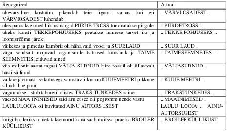
pounded words, using the hidden event LM. The er-rors are written in upper case and the correct words are written in the right column. Quick investigation reveals at least three common patterns where com-pound recomposition errors occur:
1. a compound word is not recognized when both of the compound word particles are very in-frequent: the result is that there is not enough occurrences of the pair, nor occurrences where the head word is a head in a compound, neither where the tail word is a tail in a compound; as a result, the statistical model has no reason to in-sert a compound connector between them (e.g.
piirde-tross, traks-tunkedes, ainu-autorsusest,
broiler-k¨u¨ulik)
2. two words are mistakenly recognized as a com-pound word when the first word is often a head word in compound words, and/or the second word is often a tail word in compound words, although their pair may actually never occur as a compound, and it also does not occur as an
uncompounded pair often enough (e.g. suur
laud / suur-laud,kuue meetri / kuue-meetri) 3. in some cases, words are mistakenly
recom-posed into a compound word when the fact that the words should be written separately comes
from the surrounding context (e.g. laulu looja
/ laulu-looja, kunsti tekke p˜ohjuseks / tekke-p˜ohjuseks, eri v¨arvi osadest / v¨arvi-osadest). Those errors are probably the hardest to han-dle since the correct behavior would often re-quire understanding of the discourse. Often, it is arguable whether the words should be
writ-ten as a compound or not (e.g.tekke-p˜ohjuseks,
taime-seemnetes.
Manual analysis of the compounding errors of the SpeechDat reference texts shows that the majority of
errors (around 60%) were of type 1. About 30% of the errors could be classified as context errors (type 3) and the rest (around 10%) were of type 2.
5 Conclusion
We tested two separate methods for reconstructing compound words from a stream of recognized mor-phemes, using only linguistic information. The first method, using a special compound word language model, relies on the assumption that the head part of a compound word is independent of the preceding context and its probability is calculated given only the tail. Probability of the tail, on the other hand, is calculated given the preceding context words. As an alternative approach, we proposed to use a trigram language model for locations of hidden compound word connector symbols between compound parti-cles. Experiments with two test sets showed that the method based on hidden event language model per-forms consistently better than the compound word language model based approach.
The proposed compound word reconstruction technique could be improved. The analysis of re-construction errors revealed two kinds of problems caused by data sparseness issues. Some of such is-sues could probably be eliminated by using a class-based language model. An added area for further study is to combine acoustic and prosodic cues, such as pause length, phone duration and pitch around the boundary between possible compound particles, with the linguistic model, as has been done for auto-matic sentence segmentation (Stolcke et al., 1998).
Acknowledgments
Associ-Recognized Actual
¨uhev¨arviline kost¨u¨um pikendab teie figuuri samas kui eri V ¨ARVIOSADEST l¨uhendab
.. V ¨ARVI OSADEST ..
¨ules pannakse uued liiklusm¨argid PIIRDE TROSS t˜ommatakse pingule .. PIIRDETROSS .. ¨uheks kunsti TEKKEP ˜OHJUSEKS peetakse inimese tarvet ilu ja
loomisr˜o˜omu j¨arele
.. TEKKE P ˜OHJUSEKS ..
v¨aikeses ja pimedas kambris oli n¨aha vaid voodi ja SUURLAUD .. SUUR LAUD .. v¨aga soodsalt m˜ojuvad organismile tsitrused k¨u¨uslauk ja TAIME
SEEMNETES leiduvad ained
.. TAIMESEEMNETES ..
viis miljonit aastat tagasi V ¨ALJA SURNUD hiire fossiil oli ¨ullatavalt h¨asti s¨ailinud
.. V ¨ALJASURNUD ..
vaikne ja ennast ise k¨utusega varustav liikur on KUUEMEETRI pikkune silindriline puur
.. KUUE MEETRI ..
vaguniuksel istub taburetil ˜olistes TRAKS TUNKEDES naine .. TRAKSTUNKEDES .. vaesed MAA INIMESED said aru et see oli pogromm nende vastu .. MAAINIMESED .. LAULULOOJA oli huvitatud AINU AUTORSUSEST LAULU LOOJA ..
AINU-AUTORSUSEST kuigi broileriks nimetatakse noort kana saab maitsva prae ka BROILER
K ¨U ¨ULIKUST
[image:8.595.59.524.95.365.2].. BROILERK ¨U ¨ULIKUST
Table 3: Some sample compound word reconstruction errors from the SpeechDat test set.
ation of Information Technology and Telecommuni-cations.
References
Tanel Alum¨ae. 2006.Methods for Estonian large vocab-ulary speech recognition. Ph.D. thesis, Tallinn Uni-versity of Technology.
Arvo Eek and Einar Meister. 1999. Estonian speech in the BABEL multi-language database: Phonetic-phonological problems revealed in the text corpus. In Proceedings of LP’98. Vol II., pages 529–546.
Heiki-Jaan Kaalep and Kadri Muischnek. 2005. The cor-pora of Estonian at the University of Tartu: the cur-rent situation. In The Second Baltic Conference on Human Language Technologies : Proceedings, pages 267–272, Tallinn, Estonia.
Heiki-Jaan Kaalep and Tarmo Vaino. 2001. Complete morphological analysis in the linguist’s toolbox. In Congressus Nonus Internationalis Fenno-Ugristarum Pars V, pages 9–16, Tartu, Estonia.
Einar Meister, J¨urgen Lasn, and Lya Meister. 2002. Es-tonian SpeechDat: a project in progress. InFonetiikan P¨aiv¨at 2002 — The Phonetics Symposium 2002, pages 21–26.
P. Placeway, S. Chen, M. Eskenazi, U. Jain, V. Parikh, B. Raj, M. Ravishankar, R. Rosenfeld, K. Seymore, M. Siegler, R. Stern, and E. Thayer. 1997. Hub-4 Sphinx-3 system. In Proceedings of the DARPA Speech Recognition Workshop, pages 95–100.
Vesa Siivola, Teemu Hirsim¨aki, Mathias Creutz, and Mikko Kurimo. 2003. Unlimited vocabulary speech recognition based on morphs discovered in an unsuper-vised manner. InProceedings of Eurospeech, Geneva, Switzerland.
M. Spies. 1995. A language model for compound words. InProceedings of Eurospeech, pages 1767–1779.
A. Stolcke and E. Shriberg. 1996. Automatic linguistic segmentation of conversational speech. In Proceed-ings of ICSLP, volume 2, pages 1005–1008, Philadel-phia, PA, USA.
A. Stolcke, E. Shriberg, R. Bates, M. Ostendorf, D. Hakkani, M. Plauche, G. Tur, and Y. Lu. 1998. Automatic detection of sentence boundaries and dis-fluencies based on recognized words. InProceedings of ICSLP, volume 5, pages 2247–2250, Sydney, Aus-tralia.