Knowledge-Aided Multichannel Adaptive SAR/GMTI Processing: Algorithm and Experimental Results

(1)

Volume 2010, Article ID 164187,12pages doi:10.1155/2010/164187

Research Article

Knowledge-Aided Multichannel Adaptive SAR/GMTI Processing:

Algorithm and Experimental Results

Di Wu, Daiyin Zhu, and Zhaoda Zhu

College of Information Science and Technology, Nanjing University of Aeronautics & Astronautics, Nanjing 210016, China

Correspondence should be addressed to Di Wu,wudi [email protected]

Received 30 May 2009; Revised 5 November 2009; Accepted 18 January 2010

Academic Editor: Andreas Reigber

Copyright © 2010 Di Wu et al. This is an open access article distributed under the Creative Commons Attribution License, which permits unrestricted use, distribution, and reproduction in any medium, provided the original work is properly cited.

The multichannel synthetic aperture radar ground moving target indication (SAR/GMTI) technique is a simplified implementa-tion of space-time adaptive processing (STAP), which has been proved to be feasible in the past decades. However, its detecimplementa-tion performance will be degraded in heterogeneous environments due to the rapidly varying clutter characteristics. Knowledge-aided (KA) STAP provides an eﬀective way to deal with the nonstationary problem in real-world clutter environment. Based on the KA STAP methods, this paper proposes a KA algorithm for adaptive SAR/GMTI processing in heterogeneous environments. It reduces sample support by its fast convergence properties and shows robust to non-stationary clutter distribution relative to the traditional adaptive SAR/GMTI scheme. Experimental clutter suppression results are employed to verify the virtue of this algorithm.

1. Introduction

Synthetic aperture radar (SAR) is an important sensor that can reconstruct the reflectivity image of the ground station-ary scene. Ground moving target indication (GMTI) with SAR has been widely explored for both military and civilian task. Moving target detection in SAR image is a diﬃculty, because the slowly moving target may be totally submerged among the main-beam clutter in spatial, time, and frequency domain. Space-time adaptive processing (STAP) [1–3] is a leading technology candidate for improving detection performance of airborne and spaceborne radar in strong clutter and interference environments. A simple, but of most practical importance, SAR/STAP scheme is the well-known multichannel along-track interferometric (ATI) SAR which has been widely used in the past decades [4, 5]. It utilizes two or more receiving channels whose baseline lies along the flight direction, SAR images from diﬀerent channels concerning the same scene are generated, and clutter suppression can be achieved by combining these complex images. Actually, the “combining” mentioned above can be seen as a beamforming process in image domain and the weights should be estimated adaptively from the secondary data due to the unknown characteristics of the

interference (considered to be composed of clutter and thermal noise in this paper).

It has been indicated in many literatures (e.g., [6–

8]) that STAP performance can be severely degraded in heterogeneous environments. As a simplified STAP, adaptive SAR/GMTI system is confronted with the same problem. Since the adaptive weights depend on two unknown quanti-ties, that is, the clutter-plus-noise (C+N) covariance matrix and the target steering vector, the precise estimation of the covariance matrix in heterogeneous environments presents to be a key for the detection tasks.

(2)

In this paper, we focus our research on the use of a priori knowledge in SAR/GMTI detection processing. A parametric model of multichannel SAR C +N covariance matrix is investigated at first, which can be employed as the prior form to be incorporated into the local training scheme. Based on that, a KA adaptive SAR/GMTI algorithm is proposed and verified by experimental results to be eﬀective in real-world clutter environment.

The remainder of this paper is organized as follows.

Section 2 briefly reviews the fundamental of a multichan-nel SAR detection processing and analyzes the impact of heterogeneous environments. In Section 3, a priori model of the C +N covariance matrix is formulated, and a KA adaptive SAR/GMTI algorithm is proposed to operate in the real-world clutter environments. InSection 4, experimental clutter suppression results are provided to demonstrate the desirable improvement of the proposed KA method. At last,Section 5provides a summary and conclusions. All the experimental results shown in this paper are obtained from the measured data collected by a three-channel ATI SAR system.

Notation. Vectors are denoted by boldface lowercase letters and matrices by boldface uppercase letters. We use super-scriptsT,∗, andH, to denote the transpose, conjugate and transpose conjugate operation, respectively. The Frobenius matrix norm is denoted as · and the expectation operator asE{·}.

2. Multichannel SAR/GMTI in

Heterogeneous Environments

This section develops a brief review of moving target detection flaw for a multichannel SAR system. The optimal beamforming weight vector maximizing the output signal-to-interference-plus-noise ratio (SINR) and the impact of a non-stationary clutter distribution are investigated. We validate the performance loss due to heterogeneous environ-ments using measured data taken from a three-channel SAR system.

2.1. Multichannel SAR/GMTI Detection Architecture. A mul-tichannel SAR/GMTI detection processing scheme is shown in Figure 1. SAR processing at each receiving channel is followed by a modified Σ map formation via applying a pixel-by-pixel beamforming technique between the complex maps from diﬀerent channels. By judicious setting of the beamforming weight vector, the clutter component can be filtered out, leaving only the desired targets. CFAR processing over theΣmap enables the detection of moving targets.

Consider a multichannel SAR system withK receiving channels; the returns from each transmitted pulse are received by all the channels and undergo SAR processing to produce K images. As we know, Many successful SAR imaging algorithms have been widely used [13], for example, the range-Doppler (RD), chirp scaling (CS), and omega-k algorithm, and so forth. In this paper, the polar format

algorithm (PFA) [14,15] is utilized for the images genera-tion. Thus, for a certain image pixel, there are K complex samples from diﬀerent channels, which are represented by x1,x2,. . .,xK. The beamformer input and weight vector can be represented by the K × 1 column vectors x = [x1,x2,. . . xK]T andw =[w1,w2,. . .,wK]T, respectively. The well-known optimum weight vector maximizing the output SINR is [16]

wopt=γR−1s, (1)

whereγis an arbitrary constant, andRandsare the clutter-plus-noise (C +N) covariance matrix and desired signal steering vector, respectively. In practice, due to the unknown statistics of the interference environment, the covariance matrix associated with a certain pixel is never known a priori. Thus for adaptive processing, it is common to replaceRwith its maximum likelihood estimation (MLE) [1–3]:

R= 1

L L

i=1

x(i)xH_(i). ₍₂₎

In (2),x(i) is the sample vector from the range pixel close to the pixel under test which is also called the secondary data. An important assumption for (2) is that the samples are drawn from an independent and identically distributed (i.i.d) Gaussian stochastic process. Substituting (2) into (1) yields the weight vector

w=γR−1s. (3)

The literature commonly refers to the implementation in (3) as sample matrix inversion (SMI). With this weight vector, the beamformer’s output can be represented as

xΣ=wHx. (4)

After applying the aforementioned steps for every pixel, the weightedΣmap mentioned above is formed for the next CFAR processing.

2.2. Performance Loss in Heterogeneous Environments. From (3) we note that since the inverted clutter-plus-noise covari-ance matrix is employed for weight training, the ability to accurately estimateRis decisive to a successful detection. It is clear that real-world ground clutter model will not always observe the i.i.d assumption. Variations in the underlying terrain, the intrinsic clutter motion, and the target-like signals will contribute to stationary violations [6–10]. In SAR system with high resolution, clutter properties change rapidly over image pixels. Such eﬀects lead to covariance matrix estimation errors, adaptive filter mismatch, and consequently, performance loss in GMTI processing.

(3)

channel 1 (raw data)

channel 2 (raw data)

channelK

(raw data)

SAR imaging

SAR

imaging · · ·

SAR imaging

Formation of a modifiedΣmap by beamforming

xΣ=wHx

CFAR processing (a) Detection processing flaw

SAR image 1 SAR image 2 SAR imageK

· · ·

wK

w2

w1

x1 x2 xK

xΣ

ModifiedΣmap

(b) Element-by-element beamforming

Figure1: Multichannel SAR/GMTI detection Scheme.

Table1: Parameters of the three-channel ATI SAR system.

Parameter Value

center frequency X band

antenna length 1 m

bandwidth 200 MHz

PRF 1250 Hz

number of pulses 1024

distance between each antenna

port phase center 0.33 m

platform speed 110 m/s

platform altitude 5.0 km

distance between antenna phase

center and scene center 24 km

Since we can never know exactly the trueC+Ncovariance matrix in practice, the SINR loss curve training over 64 samples with high homogeneity was superimposed here as an approximation of the real case. Note the inaccurate notch’s width, nulling placement, and insuﬃcient gains at normalized Doppler approaching −0.2∼ −0.3 for the estimated curves. Actually, the false model is a result of fast varying clutter distribution and target-like signals corrupting the secondary data. As we know, unfaithful model of SINR loss curve is tantamount to the clutter residue, target cancellation, and increasing minimum detectable velocity (MDV), which finally leads to poor detection ability of a GMTI system.

Given the impact of non-stationary clutter environments above, the traditional adaptive SAR/GMTI scheme based on the covariance matrix estimation in (2) is prone to be erroneous in heterogeneous clutter environments. It is inappropriate to consider a covariance matrix estimation method simply using (2). In the next section, a priori

knowl-−0.5 −0.4−0.3−0.2 −0.1 0 0.1 0.2 0.3 0.4 0.5 Normalised Doppler frequency

−35 −30 −25 −20 −15 −10 −5 0

SINR

loss

(dB)

64 samples 6 samples

Figure 2: Estimated SINR loss curve with diﬀerent number of training samples.

edge is introduce to construct the weight vectors, and the knowledge-aided adaptive SAR/GMTI algorithm is proposed to enhance the detection performance in heterogeneous environments.

3. Knowledge-Aided Adaptive SAR/GMTI

Knowledge-aided STAP such as colored loading and data prewhitening techniques has been proposed to enhance detection performance in heterogeneous environment [9–

(4)

CFAR, target’s velocity estimation

and relocation

(step 6) Form the KA

CMs and apply beamforming

(step 5) Form the

prior form of CMs (step 3)

Form the sample CMs

(step 4) SAR

imaging (step 2) Calibrate and

compensate the raw data (step 1) Multi-port

SAR raw data

Figure3: Knowledge-aided adaptive SAR/GMTI flow diagram.

0 100 200 300 400 500 600

Azimuth pixel 0.85

0.9 0.95 1 1.05 1.1 1.15

N

o

rm

alised

amplitude

(a) Amplitude responses before step1

0 100 200 300 400 500 600

Azimuth pixel 0.85

0.9 0.95 1 1.05 1.1 1.15

N

o

rm

alised

amplitude

(b) Amplitude responses after step1

0 100 200 300 400 500 600

Azimuth pixel −4

−3 −2 −1 0 1 2 3 4

Phase

(r

ad)

Channel 1 Channel 2

Channel 3 (c) Phase responses before step1

0 100 200 300 400 500 600

Azimuth pixel −0.5

−0.4 −0.3 −0.2 −0.1 0 0.1 0.2 0.3 0.4 0.5

Phase

(r

ad)

Channel 1 Channel 2

Channel 3 (d) Phase responses after step1

Figure4: Array responses before and after step1.

is given by a linear combination ofR0andR[17]:

R=αR0+ (1−α)R; α∈(0, 1). (5)

A method to choose α adaptively so as to maximally whiten the observed interference data is provided in [9]. Recently, new approaches for selectingαhave been proposed

in [11,12], which enable us to obtain an automatic estimate ofαdirectly from the received data set via the principle of minimum mean-squared error (MSE).

(5)

−0.5−0.4−0.3−0.2−0.1 0 0.1 0.2 0.3 0.4 0.5 Normalised Doppler frequency

−35 −30 −25 −20 −15 −10 −5 0

SINR

loss

(dB)

(a) 6 samples used

−35 −30 −25 −20 −15 −10 −5 0

SINR

loss

(dB)

(b) 12 samples used

−35 −30 −25 −20 −15 −10 −5 0

SINR

loss

(dB)

Ideal CM Sample CM

KA CM

(c) 24 samples used

Figure5: Comparison of SINR loss curves for local training and KA method.

T5 T4

T3 Road

T2

T1

Azimuth

Range

Figure6: SAR image concerning the detection area.

as an extension of the KA STAP schemes. However, it is in possession of many particular characteristics and can be conveniently implemented in practical SAR/GMTI processing.

3.1. A Priori Form of the Clutter-Plus-Noise Covariance Matrix. As the clutter-plus-noise covariance matrix is cen-tral to adaptive beamforming, we begin by building up a priori form of the multichannel SARC+Ncovariance matrix that helps motivate the KA SAR/GMTI algorithm.

Because of the two-dimensional high resolution, inter-ference present at a certain image pixel can be seen as clutter echo received from a single clutter patch plus a sampled value of thermal noise. The interference vector received on the multichannel SAR system withK receiving elements can be represented by theK×1 vector as

xI=αcc

θ,ϕεθ,ϕ1K×1+tp

θ,ϕ+n, (6)

(6)

300 350 400 450 Range index 0

5 10 15 20 25 30 35 40 45 50

Output

re

sidue

(dB)

(a) target 1

250 300 350 400

Range index 0

5 10 15 20 25 30 35 40 45 50

Output

re

sidue

(dB)

(b) target 2

150 200 250 300

Range index 0

5 10 15 20 25 30 35 40 45 50

Output

re

sidue

(dB)

(c) target 3

100 150 200 250

Range index 0

5 10 15 20 25 30 35 40 45 50

Output

re

sidue

(dB)

KA scheme SMI

(d) target 4

50 100 150 200

Range index 0

5 10 15 20 25 30 35 40 45 50

Output

re

sidue

(dB)

KA scheme SMI

(e) target 5

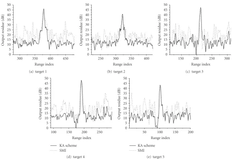
Figure7: Output residue (dB) versus range index for SMI and KA method. 24 samples are used for sample covariance matrix estimation.

or errors on the clutter signal whose characteristics may vary with angle of arrival, terrain, and so forth,1K×1is aK×1 vector of ones, andtp(θ,ϕ) is a zero-mean random vector with typically tiny variance [10,18].

We now consider the model ofC+Ncovariance matrix for multichannel SAR system, assuming that the clutter and noise vector are uncorrelated:

R=Rc+σn2IK×K, (7)

where Rc is the clutter covariance matrix, σn2 is the noise power on each channel and pixel, andIK×Kis aK×Kidentity matrix. Now considerRc with the clutter vector denoted by the first term in (6):

Rc=E αcc

θ,ϕ

×αcc

θ,ϕH

=σ2 c

cθ,ϕcH_θ,_ϕ_ε_θ,_ϕ_εH_θ,_ϕ

1K×K+Tp

θ,ϕ.

(8)

In (8),σ2

c = E[αcα∗c] denotes the clutter power concerning the discussing patch, 1K×K represents the K ×K matrix of ones, Tp(θ,ϕ) = E[tp(θ,ϕ)tHp(θ,ϕ)], and the results of

covariance matrix taper (CMT) theory [2, 19] have been invoked. It is logical to recognize that the clutter covariance matrix is comprised of a deterministic component

σ2 c

cθ,ϕcHθ,ϕεθ,ϕεH_θ,_ϕ ₍₉₎

and an unknown component

σ2 c

cθ,ϕcH_θ,_ϕ_ε_θ,_ϕ_εH_θ,_ϕ_T p

θ,ϕ. (10)

[10]. Thus, we can conclude from (7) and (8) that if the parameters, that is, σ2

c, σn2, c(θ,ϕ), and ε(θ,ϕ), at least the estimates of them, can be obtained a priori, it is not unreasonable to select

R0=σc2

cθ,ϕcHθ,ϕεθ,ϕεH_θ,ϕ₊_σ2 nIK×K,

(11)

as an initial guess ofRto be incorporated in the estimation ofC+Ncovariance matrix. Hence we concern ourselves with the problem of finding the proper values of those parameters in the following discussion.

(7)

300 350 400 450 Range index 0

5 10 15 20 25 30 35 40 45 50

Output

re

sidue

(dB)

(a) target 1

250 300 350 400

Range index 0

5 10 15 20 25 30 35 40 45 50

Output

re

sidue

(dB)

(b) target 2

150 200 250 300

Range index 0

5 10 15 20 25 30 35 40 45 50

Output

re

sidue

(dB)

(c) target 3

100 150 200 250

Range index 0

5 10 15 20 25 30 35 40 45 50

Output

re

sidue

(dB)

KA scheme SMI

(d) target 4

50 100 150 200

Range index 0

5 10 15 20 25 30 35 40 45 50

Output

re

sidue

(dB)

KA scheme SMI

(e) target 5

steering vector, as a depiction of the ULA response to a point source with direction of arrival (DoA) (θ,ϕ), takes the form

cθ,ϕ=1,ej(2πd/λ) cosθsinϕ,. . .,ej(2πd/λ)(K−1) cosθsinϕT, (12)

whereλis the radar wavelength. It is obvious that the values ofdandλare totally known before flight, and the DOA for a certain clutter path is also available via reading the records of inertial navigation unit (INU). Thus we can obtain a relative accurate value of clutter steering vector if the values of these parameters are faithful.

ε(θ,ϕ) denotes the mismatch between diﬀerent receiving channels, whose value can be derived from the actual array manifold. However, in most cases, we can never know the perfectly accurate array manifold; several measures for exploiting the clutter signal itself to estimate ε(θ,ϕ) have been proposed [18,20].

As for the noise powerσ2

n, we can use the designed signal-to-noise ratio (SNR) of a receiver as an approximation or estimate it from the minimum eigenvalue in the eigenspec-trum for a receiver test file. Besides, a simple estimation can be applied by averaging the clutter-free region in SAR image.

For estimating the clutter power σ2

c, one can utilize knowledge source as digital terrain maps, land coverage data, or stationary scene SAR images as reference. Several works have been done for these estimations; for example, paper

[9] provides a method by employing digital maps, and [21] focuses the estimation on using SAR images.

Accomplishing the replacement of all the parameters with their obtained values yields the prior form of R to be used in the KA covariance matrix estimation as (5). However, the aforementioned value obtaining process for these parameters seems to be an inconvenient work in practical processing because (1) we may not have any digital maps or SAR images before flight; the terrain information can only be acquired by theK SAR images formed in the flight; (2) the records of INU always present to be not accurate enough and lagging relative to the real values; (3) since spatial steering vector and the array errors vary with azimuth and elevation, we need to calculate them every time when process a new pixel under test. These problems motivate us to find a simple model of the prior C +N covariance matrix. As we can see in the next part, by reasonable calibrating and compensating the multichannel SAR raw data, the model of a priori clutter covariance matrix is simplified to be aK×Kmatrix of ones with a scaling scalar tantamount to the local clutter power, based on which a KA adaptive SAR/GMTI algorithm is proposed for operating in real-world environments.

(8)

300 350 400 450 Range index 0

5 10 15 20 25 30 35 40 45 50

Output

re

sidue

(dB)

(a) target 1

250 300 350 400

Range index 0

5 10 15 20 25 30 35 40 45 50

Output

re

sidue

(dB)

(b) target 2

150 200 250 300

Range index 0

5 10 15 20 25 30 35 40 45 50

Output

re

sidue

(dB)

(c) target 3

100 150 200 250

Range index 0

5 10 15 20 25 30 35 40 45 50

Output

re

sidue

(dB)

KA scheme SMI

(d) target 4

50 100 150 200

Range index 0

5 10 15 20 25 30 35 40 45 50

Output

re

sidue

(dB)

KA scheme SMI

(e) target 5

SAR system is proposed. It accomplishes GMTI processing by applying 6 major steps, which are identified by the shadowed blocks in the flow diagram ofFigure 3. The acronym CM stands for covariance matrix.

The first step involves the calibration of array errors. The mismatch between diﬀerent receiving channels is equalized by exploiting the received data itself. Several methods have been proposed for calibrating various kinds of errors in diﬀerent domains; (see [22, 23]). In our experiment, we adopt the approach mentioned in [23] to calibrate the array errors in two-dimension frequency domain and the prior form ofC+N covariance matrix corresponding to (11) as follows:

R₀=σ2 c

cθ,ϕcHθ,ϕ1K×K+εθ,ϕεHθ,ϕ

+σ2 nIK×K,

(13)

whereε(θ,ϕ) denotes the residual array error vector that can be sorted to the unknown component in (8); henceR0can be rewritten as

R₀=σ2 c

cθ,ϕcH_θ,_ϕ₊_σ2

nIK×K. (14)

As we know, since the phase lags induced by diﬀerent along track positions of receiving antenna ports can be recognized as phase response mismatch between diﬀerent receiving channels varying with DOA, they are also compen-sated in this step. Thus, the clutter steering vector for each pixel is reformatted to be aK×1 vector of ones, followed by the transformedC+Ncovariance matrix which takes the form

R0=σc21K×K+σn2IK×K. (15)

Figure 4provides the amplitude and phase responses of the three-channel SAR system before and after applying step 1 for comparison. All the response curves are normalized with respect to that of the center channel (channel 2). Therefore, a simplified form of the prior C+N covariance matrix is generated for each pixel, which is determined completely by the clutter and noise power.

In step 2, the calibrated data for each channel undergo the image formation procedure andK correlated maps are obtained for the same scenario.

Step 3 involves the construction of the prior C + N covariance matrix for each pixel. As indicated by (15), this step can be accomplished by estimating the two parameters σ2

(9)

300 350 400 450 Range index 0

5 10 15 20 25 30 35 40 45 50

Output

re

sidue

(dB)

(a) target 1

250 300 350 400

Range index 0

5 10 15 20 25 30 35 40 45 50

Output

re

sidue

(dB)

(b) target 2

150 200 250 300

Range index 0

5 10 15 20 25 30 35 40 45 50

Output

re

sidue

(dB)

(c) target 3

100 150 200 250

Range index 0

5 10 15 20 25 30 35 40 45 50

Output

re

sidue

(dB)

(d) target 4

50 100 150 200

Range index 0

5 10 15 20 25 30 35 40 45 50

Output

re

sidue

(dB)

(e) target 5

Figure10: Output residue (dB) versus range index for KA method using 6 and 24 samples, respectively.

T5 T4

T3

T2

T1

Azimuth

Range

Figure11:Σmaps formed by KA scheme with 6 samples.

methods have been used for the three-channel SAR system and equivalent results are obtained. Since the receiver noise does not change over pixels,σ2

n is estimated only once and applied to the entire image.

We consider the situation that no a priori terrain information such as digital maps and locations of man-made features is known before flight; the only knowledge source is the multichannel SAR images. Given the data compensated in the aforementioned steps, we then wish to estimate the clutter voltage of by minimizing the mean-squared error

T5 T4

T3 Road

T2

T1

Azimuth

Range

Figure12: Reposition map of control targets.

(MSE) as

min αc E

_x₋_α c1K×12

, (16)

where x denotes the input date after calibration and compensation in step 1. One of the estimated solutions to (16) takes the form

αc= 1 L_K

L₋₁

i=1

(10)

followed by the estimation of clutter power calculated by

σ2

c = |αc|2. In (17), x(i) denotes the samples vector after calibration in step 1 and L the sample number for this estimation. In order to achieve an estimation of the local clutter power with high fidelity, the samples are drawn from the closest region adjacent to the pixel under test (containing the pixel under test) and L is chosen to be small. Considering the present of targets in the sample set disturbing the estimation, the pixels which may comprise target signal should be removed. For doing this, a diﬀerence image between two images from diﬀerent channels is formed, and the image pixels whose power exceeding a predetermined threshold (20 dB above the noise floor) are censored.

After step 1∼3, a priori form ofC+Ncovariance matrix has been generated for each pixel. Step 4 is to concern the local training scheme, in which the sample covariance matrix

Rfor each pixel is estimated using (2) with the sample vectors chosen from the adjacent range pixels (including several guard cells to avoid the cancellation of moving target itself) around the pixel under test.

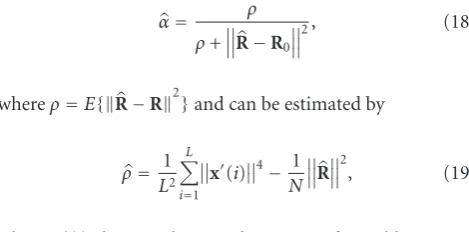
Since the prior and sample forms ofC+N covariance matrix are available after accomplishing the former steps, a linear combination of them is generated using (5) in step 5. We use the method proposed in [12] to estimate the coeﬃcientαas

α= ρ

ρ+R−R0

2, (18)

whereρ=E{R−R2}and can be estimated by

ρ= 1 L2

L

i=1

_x_(i)4₋ 1 N

R2, (19)

where x(i) denotes the samples vector after calibration in step 1. Hence the beamformer weight vectors for each pixel can be computed as

w=γR−1_s_, ₍₂₀₎

followed by the formation of the modifiedΣmap for target detection.

The last step contains CFAR processing, estimation of target’s velocity, and target relocation. Many methods have been proposed for the estimation of moving target parameters, such as monopulse [24], adaptive monopulse [24], or maximum likelihood method [25]. Since this paper does not specifically address the problem of parameters esti-mation, detailed discussion is not provided herein. However, the experimental results of radial velocity estimation and reloaction of moving target using the maximum likelihood method are shown in the next section.

3.3. Improvement for Performance Loss. To give a comparison between the KA and local training SMI scheme, Figure 5

demonstrates the benefits of utilizing a priori knowledge for

clutter suppression in multichannel SAR/GMTI processing by providing the SINR loss curves concerning the same pixel as inFigure 2for ideal, sample and linear combinationC+N covariance matrix, respectively. As we can see, by introducing the KA estimation ofR, the SINR loss curve has approached the ideal one, which is more clear for the situation of less sample support, see (a), (b). When 24 samples used, excellent coincidence can be seen between the KA and ideal curve, see (c). It can be seen that, the gap between the two methods is diminished with increasing samples which indicates that the SMI method using large number of samples may provide satisfying performance. We caution, however, adding more samples would typically degrade the sensitivity in detection targets with low radial velocities and might actually increase the chances of target-like signal falling into the samples set [6,10].

4. Experimental Results

In this section, experimental clutter mitigation results with respect to KA algorithm and traditional SMI method are presented for comparison. The data described were also collected by the three-channel SAR system with the principal parameters listed in Table 1 and a ground area including 5 control targets (cars with diﬀerent radial velocities) was imaged. Since this experiment focused on the performance of slowly moving target indication, the PRF of 1250 Hz is enough to avoid the alias of moving target in Doppler.

Figure 6provides the SAR image of the discussed scene from the central receiving channel. To identify the precise position of the road where 5 control targets were moving, several

corner reflectors had been arranged along the road before flight, which can be found in the central part of the SAR image. 5 control targets (T1∼T5) with varied radial velocities show diﬀerent azimuth displacements in the image, which are marked by the white arrows.

With SAR image generated from each receiving channel, the KA and local training SMI algorithm were applied for clutter suppression, respectively. To achieve a fair com-parison, the data were also preprocessed using Ender’s 2D calibration algorithm [23] with 1024 receiving pulses before SMI processing. We now examine how the algorithms performed against the real-world clutter environment. We first present the data as plots of output power residue (after adaptive processing) around the 5 control targets versus the range index. In each plot, a control target is at the central range gate and its return essentially extends to about 10– 15 right and left adjacent gates. Thus the data from the pixel under test and its adjacent range pixels (guard cells) are not used forC+Ncovariance matrix estimation when we adaptively process the data. The L sample vectors are formed from theL/2 data vectors associated with the range cells to the immediate right and left of the right and left guard cells, respectively. We evaluate and plot the output residue in windows (±100 range pixels) around the range pixels occupied by the 5 control targets.

(11)

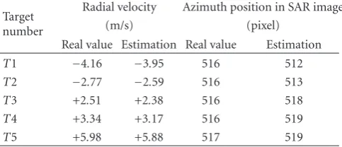
Table 2: Results of radial velocity estimation and relocation concerning the control targets.

Target number

Radial velocity Azimuth position in SAR image

(m/s) (pixel)

Real value Estimation Real value Estimation

T1 −4.16 −3.95 516 512

T2 −2.77 −2.59 516 513

T3 +2.51 +2.38 516 518

T4 +3.34 +3.17 516 519

T5 +5.98 +5.88 517 519

L, equal to 24, 12, 6, respectively. It is seen from Figure 7

(L=24) that the performance of KA method seems to have slight improvement relative to the SMI method, except that the output power of the 5th target with respect to KA method is about 5 dB better than the value with respect to SMI. For this relatively large number of samples, all the control targets are about 35 dB above the clutter power residue. For L = 12 (Figure 8), the performance of KA method is noticeably better than the SMI method in terms of the target peak to average power level outside the target gates. And forL =6 (Figure 9) there is even significant improvement of proposed KA algorithm relative to the traditional SMI method, which is on the order of 10∼15 dB. For this relatively small number of samples, the performance of KA method still seems to be graceful while the performance of local training SMI method degrades to an intolerable level that is totally unqualified for the following CFAR test.

After the comparison between clutter suppression per-formances associated with the diﬀerent algorithms, we now focus on the convergence of the proposed algorithm in heterogeneous environments. In Figure 10, we plot the output residue around the 5 control targets associated with the KA algorithm forL, equal to 24, 6, respectively. As can be seen, there is no significant performance loss when training samples decrease from 24 to 6. Acceptable clutter suppression results are achieved with less sample support for the KA algorithm, which indicated its fast convergence relative to that of SMI method.

With the beamforming applied, Figure 11 shows the modifiedΣmap formed by the KA method with 6 training samples, in which we can have an overview of the clutter mitigation performance. This map then undergoes a CA-CFAR processing and all the control targets are detected with thefalse alarmrate equal to 10−6_.

Finally, the radial velocity estimation and relocation of the detected targets is implemented.Figure 12describes the relocation result of the control targets in SAR image, in which the estimated positions are marked by the white dots. As we can see, all the targets are relocated to the azimuth positions approximately on the road. InTable 2, the detailed results of relocation as well as velocity estimation are listed, where an azimuth pixel is equal to 4.2 m and the radial velocity with “−” or “+” denotes the toward or backward motion of the control targets relative to the radar, respectively.

5. Conclusions

An eﬀective method was developed for clutter suppression of a multichannel SAR/GMTI system performs in het-erogeneous environment in this paper. It arose from the knowledge-aided STAP schemes and named as KA adaptive SAR/GMTI algorithm. In this algorithm, the prior form of C +N covariance matrix concerning each image pixel is reformed to be a K × K matrix of ones multiplied by the local clutter power plus a K ×K identity matrix multiplied by the thermal noise power. The prior form is incorporated in the estimating of the C + N covariance matrix to achieve an accurate estimate relative to the local training scheme. And then, clutter suppression beamforming is applied with the weight vector calculated by the KAC+ N covariance matrix. This new algorithm reduces sample support by its fast convergence properties and results in a clutter suppression performance that is more robust to nonstationary clutter distribution relative to the traditional scheme, which has been proved by the experimental clutter suppression results from a three-channel SAR system. These virtues make the algorithm to be an advisable choice for ground slowly moving targets detection in real-world clutter environments.

Acknowledgments

This work was supported by a Grant from the Aeronautical Science Foundation (no. 20080152004) and the Ph.D. Pro-grams Foundation of Ministry of Education of China (no. 20070280531).

References

[1] J. Ward, “Space-time adaptive processing for airborne radar,” Tech. Rep. ESC-94-109, Lincoln Laboratory, 1994.

[2] J. R. Guerci,Space-Time Adaptive Processing for Radar, Artech House, Boston, Mass, USA, 2003.

[3] R. Klemm,Principles of Space-Time Adaptive Processing, IEE Press, London, UK, 2002.

[4] E. Yadin, “Evaluation of noise and clutter induced relocation errors in SAR GMTI,” inProceedings of the IEEE International Radar Conference (RADAR ’95), pp. 650–655, Alexandria, Va, USA, May 1995.

[5] E. Yadin, “A performance evaluation model for a two port interferometer SAR-MTI,” inProceedings of the IEEE National Radar Conference, pp. 261–266, Ann Arbor, Mich, USA, May 1996.

[6] W. L. Melvin, “Space-time adaptive radar performance in heterogeneous clutter,” IEEE Transactions on Aerospace and Electronic Systems, vol. 36, no. 2, pp. 621–633, 2000.

[7] W. L. Melvin and J. R. Guerci, “Adaptive detection in dense target environments,” inProceedings of the IEEE Radar Conference, pp. 187–192, Atlanta, Ga, USA, May 2001. [8] J. S. Bergin, P. M. Techaui, W. L. Melvin, and J. R. Guerci,

“GMTI STAP in target-rich environments: site-specific anal-ysis,” inProceedings of the IEEE Radar Conference, pp. 22–25, Long Beach, Calif, USA, April 2002.

(12)

[10] J. S. Bergin, C. M. Teixeira, P. M. Techau, and J. R. Guerci, “Improved clutter mitigation performance using knowledge-aided space-time adaptive processing,”IEEE Transactions on Aerospace and Electronic Systems, vol. 42, no. 3, pp. 997–1009, 2006.

[11] X. Zhu, J. Li, and P. Stoica, “Knowledge-aided adaptive beamforming,”IET Signal Processing, vol. 2, no. 4, pp. 335– 345, 2008.

[12] P. Stoica, J. Li, X. Zhu, and J. R. Guerci, “On sing a priori knowledge in space-time adaptive processing,” IEEE Transaction on Signal Processing, vol. 56, no. 6, pp. 2598–2602, 2008.

[13] I. G. Cumming and F. H. Wong,Digital Processing of Synthetic Aperture Radar Data: Algorithms and Implementation, Artech House, Boston, Mass, USA, 2005.

[14] D. Zhu, S. Ye, and Z. Zhu, “Polar format agorithm using chirp scaling for spotlight SAR image formation,”IEEE Transactions on Aerospace and Electronic Systems, vol. 44, no. 4, pp. 1433– 1448, 2008.

[15] D. Zhu, X. Mao, Y. Li, and Z. Zhu, “Far-field limit of PFA for moving target imaging,” to appear inIEEE Transactions on Aerospace and Electronic Systems.

[16] I. S. Reed, J. D. Mallet, and L. E. Brennan, “Rapid convergence rate in adaptive arrays,”IEEE Transactions on Aerospace and Electronic Systems, vol. 10, no. 6, pp. 853–863, 1974.

[17] T. W. Anderson, An Introduction to Multivariate Statistical Analysis, John Wiley & Sons, New York, NY, USA, 2nd edition, 1984.

[18] W. L. Melvin and G. A. Showman, “An approach to knowledge-aided covariance estimation,”IEEE Transactions on Aerospace and Electronic Systems, vol. 42, no. 3, pp. 1021–1041, 2006.

[19] J. R. Guerci, “Theory and application of covariance matrix tapers for robust adaptive beamforming,”IEEE Transactions on Signal Processing, vol. 47, no. 4, pp. 985–997, 1999.

[20] W. Wirth, Radar Techniques Using Array Antennas, The Institution of Electrical Engineers, London, UK, 2001. [21] N. Goodman and P. R. Gurram, “STAP training through

knowledge-aided predictive modeling,” inProceedings of the IEEE Radar Conference, pp. 388–393, Philadelphia, Pa, USA, April 2004.

[22] M. Soumekh, “Signal subspace fusion of uncalibrated sensors with application in SAR and diagnostic medicine,” IEEE Transactions on Image Processing, vol. 8, no. 1, pp. 127–137, 1999.

[23] J. H. G. Ender, “The airborne experimental multi-channel SAR-system AER-II,” inProceedings of the European Confer-ence on Synthetic Aperture Radar (EUSAR ’96), pp. 49–52, K¨onigswinter, Germany, May 1996.

[24] U. Nickel, “Overview of generalized monopulse estimation,” IEEE Aerospace and Electronic Systems Magazine, vol. 21, no. 6, pp. 27–56, 2006.