Volume 2010, Article ID 969806,13pages doi:10.1155/2010/969806
Research Article
FPGA Implementation of the Pixel Purity Index Algorithm for
Remotely Sensed Hyperspectral Image Analysis
Carlos Gonz´alez,
1Javier Resano,
2Daniel Mozos,
1Antonio Plaza,
3and David Valencia
31Departament of Computer Architecture and Automatics, Computer Science Faculty, Complutense University of Madrid,
C/ Prof. Jos´e Garc´ıa Santesmases s/n, 28040 Madrid, Spain
2Departament of Computer Architecture, High Polytechnic Center, University of Zaragoza, C/ Mara de Luna 3, 50018 Zaragoza, Spain 3Departament of Computer Technology and Communications, Polytechnic School of C´aceres, University of Extremadura,
Avda. de la Universidad s/n, 10071 C´aceres, Spain
Correspondence should be addressed to Carlos Gonz´alez,[email protected]
Received 17 February 2010; Accepted 28 May 2010
Academic Editor: Jar Ferr Yang
Copyright © 2010 Carlos Gonz´alez et al. This is an open access article distributed under the Creative Commons Attribution License, which permits unrestricted use, distribution, and reproduction in any medium, provided the original work is properly cited.
Hyperspectral imaging is a new emerging technology in remote sensing which generates hundreds of images, at different wavelength channels, for the same area on the surface of the Earth. Over the last years, many algorithms have been developed with the purpose of finding endmembers, assumed to be pure spectral signatures in remotely sensed hyperspectral data sets. One of the most popular techniques has been the pixel purity index (PPI). This algorithm is very time-consuming. The reconfigurability, compact size, and high computational power of Field programmable gate arrays (FPGAs) make them particularly attractive for exploitation in remote sensing applications with (near) real-time requirements. In this paper, we present an FPGA design for implementation of the PPI algorithm. Our systolic array design includes a DMA and implements a prefetching technique to reduce the penalties due to the I/O communications. We have also included a hardware module for random number generation. The proposed method has been tested using real hyperspectral data collected by NASA’s Airborne Visible Infrared Imaging Spectrometer over the Cuprite mining district in Nevada. Experimental results reveal that the proposed hardware system is easily scalable and able to provide accurate results with compact size in (near) real-time, which make our reconfigurable system appealing for on-board hyperspectral data processing.
1. Introduction
Hyperspectral imaging is concerned with the measurement, analysis, and interpretation of spectra acquired from a given scene (or specific object) at a short, medium, or long distance by an airborne or satellite sensor [1]. The concept of hyperspectral imaging originated at NASA’s Jet Propulsion Laboratory in California, which developed instruments such as the Airborne Imaging Spectrometer (AIS), then called AVIRIS, for Airborne Visible Infrared Imaging Spectrometer [2]. This system is now able to cover the wavelength region from 0.4 to 2.5μm using more than two hundred spectral channels, at nominal spectral resolution of 10 nm. As a result, each pixel (considered as a vector) collected by a hyperspectral instrument can be seen as aspectral signature
or fingerprint of the underlying materials within the pixel
(seeFigure 1).
Several analytical tools have been developed for hyper-spectral data processing in recent years, covering topics like dimensionality reduction, classification, data compression, or spectral mixture analysis [3]. The underlying assumption governing clustering and classification techniques is that each pixel vector comprises the response of a single underlying material. However, if the spatial resolution of the sensor is not high enough to separate different materials, these can jointly occupy a single pixel and the resulting spectral measurement will be amixedpixel, that is, a composite of the individual pure spectra. For instance, inFigure 1it is likely that the pixel labeled as “vegetation” is actually a mixture of vegetation and soil, or of different types of vegetation canopies.
2400 2000 1600 1200 800 400
Wavelength (nm) 0
0.2 0.4 0.6 0.8 1
Re
fl
ec
ta
n
ce
2400 2000 1600 1200 800 400
Wavelength (nm) 0
0.2 0.4 0.6 0.8 1
Re
fl
ec
ta
n
ce
2400 2000 1600 1200 800 400
Wavelength (nm) 0
0.2 0.4 0.6 0.8 1
Re
fl
ec
ta
n
ce
2400 2000 1600 1200 800 400
Wavelength (nm) 0
0.2 0.4 0.6 0.8 1
Re
fl
ec
ta
n
ce
Atmosphere
Soil
Water
Vegetation
Figure1: The concept of hyperspectral imaging.
analysis terminology [5] and then express the measured spectrum of each mixed pixel as a linear combination of endmembers weighted by fractions or abundances that indicate the proportion of each endmember present in the pixel. In fact, spectral mixture analysis has been an alluring exploitation goal since the earliest days of hyperspectral imaging [4]. No matter the spatial resolution, in natural environments the spectral signature for a nominal pixel is invariably a mixture of the signatures of the various materials found within the spatial extent of the ground instantaneous field view of the sensor. In hyperspectral imagery, the number of spectral bands usually exceeds the number of pure spectral components and the unmixing problem is cast in terms of an overdetermined system of equations in which given the correct set of end-members allows determination of the actual endmember abundance fractions through a numerical inversion pro-cess.
Let us assume that a remotely sensed hyperspectral scene with N bands is denoted by F, in which a pixel at
discrete spatial coordinates is represented by a vector f =
[f1,f2,. . .,fN], where fkdenotes the spectral response at the
kth wavelength, withk=1,. . .,N. Under the linear mixture model assumption, each pixel vector in the original scene can be modeled using the following expression:
f= E
i=1
ai·ei+n, (1)
whereeidesignates the ith pure spectral component
(end-member) residing in the pixel,aiis a scalar value designating
the fractional abundance of the endmembereiat the pixel f,E is the total number of endmembers, and n is a noise vector. The solution of the linear spectral mixture problem described in (1) relies on the correct determination of a set
{ei}E
i=1 of endmembers. It is such derivation and validation
Skewer 2
Skewer 3 Skewer 1
Extreme pixel Extreme
pixel Extreme
pixel
Extreme pixel
Figure 2: Toy example illustrating the performance of the PPI endmember extraction algorithm in a 2-dimensional space.
The pixel purity index (PPI) algorithm [7] has been widely used in hyperspectral image analysis for endmem-ber extraction due to its publicity and availability in ITTVIS (http://www.ittvis.com/) Environment for Visualiz-ing Images (ENVIs) software originally developed by Ana-lytical Imaging and Geophysics (AIGs) [8]. The algorithm searches for a set of vertices of a convex hull in a given dataset, which are supposed to be pure signatures present in the data. Due to its propriety and limited published results, its detailed implementation has never been made publicly available. Therefore, most of the people who use the PPI for endmember extraction either appeal for ENVI software or implement their own versions of the PPI based on whatever available in the literature. The general procedure of the PPI algorithm can be summarized as follows [9].
(1) First, a pixel purity score is calculated for each pixel vectorf in the input hyperspectral image cubeFby generatingKrandom,N-dimensional vectors, called
skewers.
(2) Then, each pixel vectorfin the input data is projected onto the entire set of skewers {skewerj}Kj=1, and
the pixels falling at the extremes of each skewer are tallied (seeFigure 2). After many repeated projections to different random skewers, those pixels which are repeatedly selected during the process are identified and placed on a list of endmember candidates. (3) The potential endmember spectra are then loaded
into an interactive tool (such as ENVI’s N -dimensional visualizer, available as a built-in com-panion piece in ENVI software) and rotated until a desired number of endmembers are visually identi-fied as extreme pixels in the data cloud.
The PPI algorithm suffers from several limitations [10]. First and foremost, the algorithm is sensitive to parameter
K, that is, the number of skewers. Since the skewers are randomly generated, a large number of skewer projections are generally required in order to arrive to satisfactory
endmember sets in terms of signature purity. The authors recommend using as many random skewers as possible in order to obtain optimal results [7]. As a result, the PPI can only guarantee to produce optimal results asymptotically and its computational complexity is very high, thus requiring efficient implementations. Another shortcoming of the PPI is the fact that an interactive tool is needed to perform the final endmember selection. An alternative is to retain the pixels that have been selected above a predefined threshold and then automatically remove spectrally redundant endmem-bers [10]. This is generally treated as a postprocessing stage external to the algorithm.
An exciting new development in the field of specialized commodity computing for accelerating computationally intensive algorithms is the emergence of hardware devices such as field programmable gate arrays (FPGAs) [11–13], which can bridge the gap towards on-board and real-time analysis of remote sensing data [14, 15]. FPGAs are now fully reconfigurable [16, 17], a technological feature that, in our application context, allows a control station on Earth to adaptively select a data processing algorithm (out of a pool of available algorithms implemented on the FPGA) to be applied on board the sensor. The ever-growing computational demands of hyperspectral imaging applications can fully benefit from compact, reconfigurable hardware components and take advantage of the small size and relatively low cost of these units.
In this paper, we develop an FPGA-based hardware version of the PPI algorithm. The proposed implementa-tion is aimed at enhancing code reusability and efficient implementation in FPGA devices through the utilization of systolic array design. One of the main advantages of systolic array-based implementations is that they are able to provide a systematic procedure for system design that allows for the derivation of a well-defined processing element-based structure and an interconnection pattern which can then be easily ported to real hardware configurations. The remainder of the paper is organized as follows. Section 2 discusses the role of reconfigurable hardware in remote sensing missions.Section 3describes our implementation of the PPI algorithm.Section 4describes its parallel implementation on a Xilinx Virtex-II PRO xc2vp30 FPGA. Section 5 provides an experimental assessment of both endmember extraction accuracy and parallel processing performance of the pro-posed FPGA-based algorithm, using a well-known hyper-spectral data set (with quality ground-truth) collected by the NASA Jet Propulsion Laboratory’s Airborne Visible Infrared Imaging Spectrometer (AVIRIS) [2] over the Cuprite mining district in Nevada. Finally, Section 6 concludes with some remarks and hints at plausible future research lines.
2. The Role of Reconfigurable Hardware in
Remote Sensing Missions
The trend in remote sensing missions has always been towards using hardware devices with smaller size, lower cost, more flexibility, and higher computational power [18,
reutilization of expensive hardware resources. Instead of storing and forwarding all captured images, remote sensing data interpretation can be performed on orbit prior to downlink, resulting in a significant reduction of communi-cation bandwidth as well as simpler and faster subsequent computations to be performed at ground stations. In this regard, FPGAs combine the flexibility of traditional micro-processors with the power and performance of application-specific integrated circuits (ASICs). Therefore, FPGAs are a promising candidate for on-board remote sensing data processing.
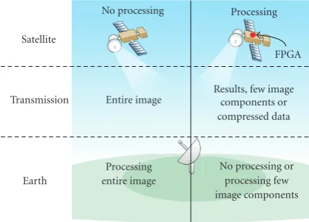
Figure 3illustrates some potential advantages of using reconfigurable hardware in remote sensing data processing. The transmission of high-dimensional information collected by a satellite-based instrument to a control station on Earth for subsequent processing may turn into a very slow task, mainly due to the reduced bandwidth available and to the fact that the connection may be restricted to a short period of time. The ability to interpret remote sensing data on-board can significantly reduce the amount of bandwidth and storage space needed in the generation of science products. Subsequently, on-board processing has the potential to reduce the cost and the complexity of ground control systems. Furthermore, it allows autonomous decisions (to be taken on board) that can potentially reduce the delay between image capture, analysis, and action.
Recently, FPGAs have become a viable target technol-ogy for implementation of remotely sensed hyperspectral imaging algorithms [20]. These computing systems combine the flexibility of general purpose processors with the speed of application-specific processors. Reconfigurable hardware offers the necessary flexibility and performance with reduced energy consumption compared to other high performance processors. By mapping functionality to FPGAs, the com-puter designer can optimize the hardware for a specific application resulting in acceleration rates of several orders of magnitude over general-purpose computers. In addition, these devices are characterized by lower form/wrap factors compared to parallel platforms and by higher flexibility than ASIC solutions. Reconfigurable computing technology further allows new hardware circuits to be uploaded via a radio link for physical upgrade or repair [21].
Moreover, satellite-based remote sensing instruments can only include chips that had been certified for space conditions. This is because space-based systems must operate in an environment in which radiation effects have an adverse impact on integrated circuit operation [22]. Ionizing radia-tion can cause soft-errors in the static cells used to hold the configuration data. This will affect the circuit functionality and can cause system failure. So it requires special FPGAs that provide on-chip reconfiguration error-detection and/or correction circuitry. High-speed, radiation-hardened FPGA chips with million gate densities have recently emerged that can support the high throughput requirements for the remote sensing applications. Radiation-hardened FPGAs are in great demand for military and space applications. For instance, industrial partners such as Actel Corporation (http://www.actel.com/) or Xilinx (http://www.xilinx.com/) have been producing radiation-tolerant antifuse FPGAs for
several years for high-reliability space-flight systems. Actel FPGAs have been on board more than 100 launches and Xilinx FPGAs have been used in more than 50 missions [22]. In this work, we use a Xilinx Virtex-II PRO xc2vp30 FPGA as a baseline architecture because it is similar to other FPGAs [23] that have been certified by several international agencies for remote sensing applications. They are based on the same architecture so we could immediately implement our design on them.
3. The Pixel Purity Index (PPI) Algorithm
Since the details of the specific steps to implement ENVI’s PPI are not available in the literature, the PPI algorithm described below is only based on the limited published results and our own interpretation [10]. Nevertheless, except a final manual supervision step (included in ENVI’s PPI) which is replaced by step 4, both our approximation and the PPI in ENVI 4.0 produce very similar results. The inputs to the algorithm are a hyperspectral data cube F with N
dimensions; the number of random skewers to be generated during the process,K; and a cut-offthreshold value,tv, used
to select as final endmembers only those pixels that have been selected as extreme pixels at leasttvtimes throughout the PPI
process.
The algorithm is given by the following steps.
(1)Skewer generation. Produce a set of K randomly
generated unit vectors{skewerj}K j=1.
(2)Extreme projections. For eachskewerj,j= {1,. . .,K},
all pixel vectorsfiin the original data setFare
pro-jected ontoskewerjvia dot products of|fi·skewerj|
to find sample vectors at its extreme (maximum and minimum) projections, thus forming an extrema set for skewerj which is denoted by Sextrema(skewerj).
Despite the fact that different skewers generate dif-ferent extrema sets, it is very likely that some sample vectors may appear in more than one extrema set. To account for this, we define an indicator function of a setF, denoted byIS(x), to denote membership of an
elementxto that particular set as follows:
IS(x)=
1 ifx∈S 0 ifx∈/S
, (2)
(3)Calculation of PPI scores. Using the indicator function
above, we calculate the PPI score associated to each pixel vectorfi(i.e., the number of times that a given
pixel has been selected as extreme in step 2) using the following equation:
NPPI(fi)= k
j=1
ISextrema(skewerj)(fi), (3)
(4)Endmember selection. Find the pixel vectors with
scores ofNPPI(fi) which are abovetvand label them
Satellite
Transmission
Earth
No processing
Entire image
Processing entire image
Processing
FPGA Results, few image
components or compressed data
No processing or processing few image components
Figure3: Potential advantages of using reconfigurable hardware in remote sensing data processing.
The most time-consuming stage of the PPI algorithm is stage 2 (extreme projections). For example, running this stage on a hyperspectral image with 614×512 pixels (the standard number of pixels produced by NASA’s AVIRIS instrument in a single frame, each with 224 spectral bands) usingK=400 skewers requires the calculation of more than 2 × 10¹¹ multiplication/accumulation (MAC) operations,
that is, a few hours of nonstop computation on a 500 MHz microprocessor with 256 Mbytes SDRAM [24,25]. In [20], another example is reported in which the PPI algorithm available in ENVI 4.0 version took more than 50 minutes of computation to project every data sample vector of a hyperspectral image with the same size reported above onto 104skewers in a PC with AMD Athlon 2.6 GHz processor and
512 MB of RAM.
Fortunately, the PPI algorithm is well suited for parallel implementation. The computation of skewer projections is independent and can be performed simultaneously, leading to many ways of parallelization. In [24, 25], two parallel architectures for implementation of the PPI are proposed. Both are based on a 2D processor array tightly connected to a few memory banks. A speedup of 80 is obtained through an FPGA implementation on the Wildforce board (4 Xilinx XC4036EX plus 4 memory banks of 512 Kbytes) [26]. As a matter of fact, this design is tailored to the Wildforce board and it cannot be reused for another board without huge modifications. In [10], a fast iterative PPI (FPPI) is introduced. The Matlab-based software implementation of the FPPI algorithm was more than 24 times faster than the ENVI’s PPI algorithm in the same computing environment, while the FPGA-based implementation showed a significant increase in performance with regards to the two considered software versions due to the low-level hardware implementa-tion. Although these works have demonstrated the efficiency of a hardware implementation on a reconfigurable board, these solutions are not scalable.
The FPGA implementation that we present in the follow-ing section aims at overcomfollow-ing these drawbacks. First, our architecture specification can be easily adapted to different
platforms. Second, our proposed architecture is scalable depending on the amount of available resources because the required resources grow proportionally with the number of skewers and the clock cycle remains constant.
4. FPGA Implementation
4.1. Parallel Design Strategies for the PPI Algorithm. The
most time-consuming stage (extreme projections) of the PPI computes a very large number of dot products, all of which can be performed simultaneously. If we consider a simple dot-product unit such as the one displayed inFigure 4(a)as the baseline for parallel computations, then we can perform the parallel computations by pixels (see Figure 4(b)), by skewers (see Figure 4(c)), or by pixels and skewers (see
Figure 4(d)). If we parallelize the computations by pixels, additional hardware is necessary to compare all the maxima and minima between them. As we increase the number of parallel computations, a greater area would be required for maxima/minima computations and the critical path would be longer, hence, the clock cycle would be higher. Another possible way to parallelize the extreme projections stage is to computeK dot products at the same time for the same pixel, whereKis the number of skewers (seeFigure 4(c)). If we increase the number of skewers in this case, the required area would grow proportionally with the number of dot-product units and the clock cycle would remain constant. Finally, the parallelization strategy inFigure 4(d)is a mixed solution which provides no further advantage with respect to the parallelization by skewers and has the same problems that parallelization by pixels has.
Taking in mind the above rationale, in this work we have selected the parallelization strategy based on skewers. Apart from the aforementioned advantages with regard to other possible strategies, another reason for this selection is that the parallelization strategy based on skewers fits very well how the image data reaches the system. In our case, our goal is to make an on-line processing of the hyperspectral images bearing in mind that hyperspectral sensors capture the image data in a pixel by pixel fashion. Therefore, parallelization by skewers is the one that best fits the data entry mechanism since each pixel can be processed immediately as collected. Specifically, our hardware system should be able to compute
K dot products at the same time against the same pixelfi,
where K is the number of skewers. In such a system, the
extreme projectionsstep of the PPI (the most time-consuming
one in the PPI process) can be simply written as described in
Algorithm 1.
The par loop in Algorithm 1 expresses that K dot products are first performed in parallel, then K Min and Max operations are also computed in parallel. Now, if we suppose that we cannot simultaneously compute K dot products but only a fractionK/P, whereK/Pis the number of available processing units in the underlying parallel platform, then theextreme projectionsstep can be split intoP passes, each performing T × K/P dot products, as indicated in
Pixel
Skewer
Dot max
min (a) dp unit
Pixel 1 Skewer
Dot max min
· · ·
Pixeln
Skewer Dot
max min
max min Max/Min
(b) pixels
Pixel
Skewer 1 Dot
max min .
.
. Pixel
Skewerk
Dot max min (c) skewers
. . .
Pixel 1 Skewer 1
Dot · · ·
Pixeln
Skewerk
Dot
max min
Max/Min Pixel 1
Skewerk
Dot
max min
max min
· · ·
Pixeln
Skewer 1
Dot
max min
Max/Min
max min
max min (d) skewers and pixels
Figure4: (a) Dot-product (dp) unit. (b) Parallelization strategy by pixels. (c) Parallelization strategy by skewers. (d) Parallelization strategy by skewers and pixels.
for(f =0;f < F;f++){//Fdenotes the number of pixels
par(k=0;k < K;k++){//Kdenotes the number of skewers dp[k]=dot product(pixels[f],skewers[k]);
if (dp[k]<Min[k]){Min[k]=dp[k]; Reg Min[k]=f;}
if (dp[k]>Max[k]){Max[k]=dp[k]; Reg Max[k]=f;} }end par
}end for
Algorithm1: Parallel implementation ofextreme projectionsstep.
processor receives successively theTpixels, computesT dot-products, and keeps in memory the Min and the Max dot products. In this scheme, each processor holds a different skewer which must be input before each new pass.
To conclude this section, we would like to emphasize the advantages of the considered parallelization strategy over other possible alternatives. For this purpose, Figure 5
compares the three parallelization strategies in Figure 4: parallelization by pixels (seeFigure 4(b)), parallelization by skewers (seeFigure 4(c)), and parallelization by skewers and pixels (seeFigure 4(d)). The different parallel design strate-gies for the PPI algorithm have been described using VHDL language and we have used the Xilinx ISE environment to implement them and obtain the necessary resources (see
Figure 5(a)) and the clock cycle (seeFigure 5(b)) in each of the three parallelization strategies for the same number of dot-processing units. Once all the designs were implemented we measured their performance with clock-cycle accuracy.
As shown in Figure 5, parallelization by skewers offers significant advantages with regards to the other considered implementation strategies.
4.2. Hardware Implementation. Figure 6shows the
architec-ture of the hardware used to implement the PPI algorithm, along with the I/O communications. For data input, we use a DDR2 SDRAM and a DMA (controlled by a PowerPC) with a Write FIFO to store pixel data. A Read FIFO and a transmitter are used to send the endmembers via an RS232 port. Finally, a systolic array and a random generation module are used to implement our version of the PPI algorithm.
for(p=0;p < P;p++){//Pis the number of algorithm iterations
x=p×(K/P); //Kdenotes the number of skewers
for(f =0;f < F; f++){//Ndenotes the number of pixels
par(k=0;k < K/P;k++){
dp[x+k]=dot product(pixels[f],skewers[x+k]);
if (dp[x+k]<Min[x+k]){Min[x+k]=dp[x+k]; Reg Min[x+k]=f;}
if (dp[x+k]>Max[x+k]){Max[x+k]=dp[x+k]; Reg Max[x+k]=f;} }end par
}end for }end for
Algorithm2: Parallel implementation ofextreme projectionsstep (rewritten to be split intoPalgorithm iterations).
Area required
100 90 80 70 60 50 40 30 20 10
(dp) units Skewers
Pixels
Pixels and skewers 0
2000 4000 6000 8000 10000 12000 14000
Slic
es
(a)
Frequency
100 90 80 70 60 50 40 30 20 10
(dp) units Skewers
Pixels
Pixels and skewers 0
20 40 60 80 100 120 140 160 180 200
(MHz)
(b)
Figure5: (a) Area required (in slices) by dot-processing units in different parallel implementation strategies of the PPI. (b) Clock cycle required (in MHz) by dot-processing units in different parallel implementation strategies of the PPI.
FPGA
Systolic array
C.U. DMA
Read FIFO
Write FIFO POWERPC
DDR2 SDRAM RS232
Read
Empty FIFO Endmember
Read Write
Calculate Next End image
Transmitter
Next slot
Endmember
Occupancy Write Seed
Seed End pixel
Random
generation of skewers End pixel
Pixel data
Nthcomponent of each skewer
Pixel Skewer
(dp) unit
C.U.
End pixel Calculate
min index
max index min/max unit
+/− <
>
Figure7: Hardware architecture of a dot-product processor.
of N spectral values, just like a skewer. A dot-product calculation between a pixelfi and askewerj can be simply
obtained by using the expression Nk=1fi(k) × skewer(jk).
Therefore, a full vector dot-product calculation requiresN
multiplications andN−1 additions, whereNis the number of spectral bands. As it was shown in previous work [25], the skewer values can be limited to a very small set of integers when N is large, as in the case of hyperspectral images. A particular and interesting set is {1,−1} since it avoids the multiplication. The dot product is, thus, reduced to an accumulation of positive and negative values. With the above assumptions in mind, each dot-product processor only needs to accumulate the positive or negative values of the pixel input according to the skewer input. These units are, thus, only composed of a single addition/subtraction operator and a register. The Min/Max unit receives the result of the dot product and compares it with the previous minimum and maximum values. If the result is a new minimum or maximum, it will be stored for future comparisons together with its corresponding index. For simplicity, the part related to the management of indexes has been omitted inFigure 7.
Taking into account that the latency of an addition or a subtraction is just one clock cycle, then the calculation of a dot product requiresN+ 1 clock cycles. In each cycle, the processor sequentially receives the data of a pixel and accumulates the result, adding or subtracting, depending on the skewer component. The additional clock cycle is required for the comparison with a max and a min value and the pixel updating. We have evaluated different options to remove the last clock cycle, but finally we have decided to keep it. One option was to update the min and max indexes in parallel with the computation of the next dot product, but it requires a more complex hardware mechanism (at least two more registers) and makes this solution worse globally because we can synthesize less systolic processors on the FPGA. We can also update the pixel during the last clock cycle of each systolic cycle, but it increases the critical path and increases the clock frequency. Hence, whenNis a large number (as in the case of hyperspectral images), we obtain higher computation times.
One of the main features of our system is the incor-poration of a hardware-based random generation module that significantly reduces the I/O communications that,
End pixel Next Seed 1 Seed 2 End image
Random generation module
XOR nthcomponent of each skewer
<<
Figure8: Hardware architecture of the random number generation module.
Power PC DMA
DDR2 SDRAM
Write FIFO
Read FIFO Systolic
array
RS232 transmitter
Random
generation Stage 2
Stage 1 Stage 3
Figure9: Our pipeline architecture.
in previous implementations of the PPI, were the main bottleneck [20,24,25]. Previous works presented in [25,27,
28] use the concept of the so-called block of skewers (BOSs) to generate the skewers. The idea of the BOS method is first to randomly generateBunit vectors, called independent skewer (Iskewers){Iskewerb}Bb=1 and then use them as a building
blocks to generate the remaining skewers, called dependent skewers (Dskewers). The Dskewers are linear combination of theB Iskewers. The goal of this approach is to reduce the number of dot products needed. The difference between the BOS method and the PPI is that the former uses the Dskewers to implement the PPI, while the skewers used in the latter are independently generated randomly. The work presented in [27] also analyses possible ways to further reduce the number of dot products and proposes to use FPGAs for the dot-products computations. In this work, we have implemented a random generator module similar to the one presented in [29]. This module provides pseudo-random and uniformly-distributed sequences using registers and XOR gates.Figure 8
shows the structure of the random generation module. It has two registers to store the new seeds. These seeds are initialized by the system each time that the PPI algorithm computes the image. At the beginning of every systolic cycle, we also store these two seeds in the other two registers. This generator reduces the number of resources needed because we do not need to store theNbits ofKskewers, but onlyK
bits of two seeds. It requires an affordable amount of space (288 slices for 100 skewers) and it is able to generate the next component of every skewer in only one clock cycle and operates at a high clock frequency (664 MHz).
To conclude this section, we provide a step-by-step description of how the proposed architecture performs the extraction of a set of endmembers from a hyperspectral image.
(i) Firstly, to initialize the random generation module, the PowerPC generates two seeds of K bits (where
Kis the number of skewers) and writes them to the Write FIFO.
(ii) Afterwards, the control unit reads these seeds and sends them to the random generation module where they are stored. Hence, the random generation module can provide the systolic array with one bit for each skewer every clock cycle as we have described in this section.
(iii) After the PowerPC has written the two seeds, it sends an order to the DMA to start copying a piece of the image from the DDR2 SDRAM to the Write FIFO. As mentioned before, the main bottleneck in this kind of system is frequently the data input which is addressed in our implementation by the incorporation of a DMA that eliminates most I/O overheads. Moreover, the PowerPC monitors the input FIFO and sends a new order to the DMA every time that it detects that the Write FIFO is half empty. This time, the DMA will bring a piece of the image that occupies half of the Write FIFO total capacity.
(iv) When the data of the first pixel have been written in the Write FIFO, the systolic array and the random generation module start working. Every clock cycle, a new pixel is read by the control unit and sent to the systolic array. In parallel, thekth component of each skewer also is sent to the systolic array by the random generation module.
(v) DuringNclock cycles, data of a pixel are accumulated positively or negatively depending of the skewer component. In the next clock cycle, the Min/Max unit updates the pixel and the random generation module restores the original two seeds, concluding the systolic cycle. In order to process the hyperspec-tral image, we need as many systolic cycles as pixels in the image. When the entire image is processed, the control unit writes the endmembers to the Read FIFO.
(vi) Finally, the Transmitter extracts the endmembers from the Read FIFO and sends them via an RS232 port.
(vii) These steps are repeated several times depending on the number of skewers we can parallelize and the number of skewers we want to evaluate.
5. Experimental Results
5.1. FPGA Architecture. The hardware architecture described
in Section 4 has been implemented using VHDL language for the specification of the systolic array. Further, we have
used the Xilinx ISE environment and the Embedded Devel-opment Kit (EDK) environment (http://www.xilinx.com/ise/ embedded/edk pstudio.html) to specify the complete sys-tem. The full system has been implemented on an XUPV2P board, a low-cost reconfigurable board with a single Virtex-II PRO xc2vp30 FPGA component, a DDR SDRAM DIMM slot which holds up to 2 GBytes, an RS232 port, and some additional components not used by our implementation.
5.2. Hyperspectral Data. The hyperspectral dataset used
in these experiments is the well-known AVIRIS Cuprite scene (seeFigure 10(a)), available online in reflectance units (http://aviris.jpl.nasa.gov/html/aviris.freedata.html). This scene has been widely used to validate the performance of endmember extraction algorithms. The scene comprises a relatively large area (350 lines by 350 samples and 20-m pixels) and 224 spectral bands between 0.4 and 2.5μm, with nominal spectral resolution of 10 nm. Bands 1–3, 105–115, and 150–170 were removed prior to the analysis due to water absorption and low SNR in those bands. The site is well understood mineralogically and has several exposed minerals of interest including alunite, buddingtonite, calcite, kaolinite, and muscovite. Reference ground signatures of the above minerals (seeFigure 10(b)), available in the form of a US Geological Survey library (USGS) (http://speclab.cr.usgs.gov/spectral-lib.html), will be used to assess endmember signature purity in this work.
5.3. Endmember Extraction Accuracy Evaluation. Before
ana-lyzing the parallel properties of the proposed implemen-tation, we first conducted an experiment-based cross-examination of endmember extraction accuracy to assess the spectral similarity between the USGS library spectra and the corresponding endmembers extracted by the considered implementation of the PPI algorithm. Table 1 shows the spectral angle distance (SAD) [3] between the most similar endmembers detected by the original ENVI implementation (using the supervised N-dimensional visualization tool to derive the final set of endmembers), the PPI approximation described inSection 3(implemented in the C++ program-ming language), and our FPGA-based implementation. In all cases, we usedK =104skewers which provided the best
compromise (after testing a wide range of values) and thus set the threshold valuetvto the mean ofNPPIscores obtained
afterK = 104 iterations. It should be noted that the SAD
between a pixel vectorfiselected by the PPI and a reference
spectral signaturesjis given by
SADfi,sj
=cos−1 fi·sj
fi·sj.
(4)
(a)
2500 2200 1900 1600 1300 1000 700 400
Wavelength (nm) Alunite
Kaolinite
Buddingtonite
Muscovite
Calcite
0.2 0.4 0.6 0.8 1
Re
fl
ec
ta
n
ce
(b)
Figure10: (a) False color composition of the AVIRIS hyperspectral over the Cuprite mining district in Nevada. (b) US Geological Survey mineral spectral signatures used for validation purposes.
Table1: Spectral angle-based similarity scores between the end-members extracted by different implementations of PPI and the selected USGS reference signatures.
USGS ENVI PPI Our FPGA-based
mineral software approximation PPI
Alunite 0.084 0.084 0.084
Buddingtonite 0.071 0.068 0.068
Calcite 0.089 0.089 0.089
Kaolinite 0.136 0.132 0.132 Muscovite 0.092 0.081 0.081
is because ENVI’s PPI implementation includes a manual supervision procedure to select the final endmembers and, hence, it is user dependent. In our experiments with theN -dimensional visualization tool available in ENVI, we made sure to perform many interactive rotations in order to select the best possible endmembers. In any event, both our PPI approximation inSection 3and the FPGA implementation inSection 4produced very similar results to those found by ENVI’s PPI, but in a fully automatic fashion.
5.4. Parallel Performance Evaluation. Table 2 shows the
resources used for our hardware implementation of the proposed PPI algorithm design for different numbers of skewers (ranging from K = 20 to K = 100), tested on the Virtex-II PRO xc2vp30 FPGA of the XUPV2P board. This FPGA has a total of 13696 slices, 27392 slice flip flops, and 27392 four-input LUTs available. In addition, the FPGA includes some heterogeneous resources, such as two PowerPCs and distributed Block RAMs. In our implemen-tation, we took advantage of these resources to optimize the design. One PowerPC monitors the communications and the Block RAMs are used to implement the FIFOs, so the vast majority of the slices are used for the implementation of
the PPI algorithm. As shown byTable 2, we can scale our design up to 100 skewers (therefore, P = 100 algorithm passes are needed in order to process K = 104 skewers).
An interesting feature of our systolic array design is that we can scale it without increasing the delay of the critical path. Hence, the clock cycle remains constant at 187 MHz. Compared with the FPGA implementation of the FPPI algorithm presented in [20], our systolic array uses half of the slices and its clock frequency is 10 times higher. It should be noted that, in the current implementation, the complete AVIRIS hyperspectral image is stored in an external DDR2 SDRAM.Table 3shows its characteristics. However, with an appropriate controller, other options could be supported, such as using flash memory to store the hyperspectral data.
Table2: Summary of resource utilization for the FPGA-based implementation of the PPI algorithm.
Component Number of skewers
Number of slice flip flops
Number of 4 input LUTs
Number of slices
Percentage of total
Maximum operation frequency (MHz)
Systolic Array
20 2240 3865 2085 15.22 187
40 4480 7728 4170 30.44 187
60 6720 11591 6254 45.66 187
80 8960 15454 8339 60.88 187
100 11200 19317 10423 76.1 187
Random Generation Module
20 40 120 58 0 664
40 80 240 115 0.42 664
60 120 360 173 0.84 664
80 160 480 230 1.68 664
100 200 600 288 2.1 664
RS232 Transmitter — 69 128 71 0.52 208
DMA Controller — 170 531 367 2.68 102
Table3: Characteristics of the SDRAM memory module used to store the hyperspectral data.
Memory Module Memory Organization Number of Ranks Registered or Unbuffered CAS Latency
KVR266X64C25/512 512 MB 64 M×64 Dual Unbuffered 2.5
Table4: Comparison of different implementations of the PPI algorithm.
Algorithm PPI Approximation FPGA implementation in [20] Proposed FPGA implementation
Processing time (seconds) 3068 62 31
penalties due to reading of the input data. To demonstrate the advantages of using a DMA, we have developed another version in which the image data are read from memory and written to the Write FIFO by the PowerPC instead of the DMA. In this version, the processing time was increased more than an order of magnitude (340 seconds) so we can conclude that the resources used for the DMA (621 slices) are well spent.
For illustrative purposes, we have performed a compari-son of our proposed FPGA design with previous implemen-tations in terms of computation time. As mentioned above, our FPGA-based implementation of the PPI algorithm can handle up to 100 skewers in parallel. Since K =
104, the complete image has been processed P = 100
times.Table 4shows the computing time for three different implementations: our PPI approximation in Section 3, an FPGA-based implementation presented in [20], and the FPGA-based implementation proposed in Section 4of this paper. The PPI approximation was implemented in an AMD Athlon 2.6 GHz processor with 512 MB of RAM. The FPGA-based implementation in [20] was implemented in a Xilinx Virtex-II XC2V6000-6 FPGA with 33792 slices available. Finally, our proposed FPGA implementation was implemented on a Xilinx Virtex-II PRO xc2vp30 FPGA with 13696 slices available. As shown byTable 4, the FPGA-based implementation in [20] was more than 49 times faster than the PPI approximation for the AVIRIS Cuprite image, while
our FPGA implementation of the PPI shows a significant increase in performance with regards to the FPGA-based implementation in [20], with a speedup of 2 with regard to that implementation. We must consider that the FPGA used in [20] has 2.5 times more slices than the one used in our implementation of the PPI algorithm. Furthermore, it is worth noting that we used a clock of 100 MHz (the maximum frequency available in EDK 9.1 for the Processor Local Bus [30]) for the calculation of the dot products. Therefore, we believe that there is still room for further improvements of the achieved computation time in future developments.
To conclude this section, we would like to show the execution time evolution as we increase the number of parallel dp units to calculate a fixed number of projections (104).Figure 11shows this evolution. We must consider that
this behavior depends on the number of times we have to process the full image and therefore we are not always calculating 104 projections. For example, if we have 90 dp
units in parallel, we need almost 112 algorithm passes to calculate 104projections or more, so we are really calculating
122×90=10080 projections.
6. Conclusions and Future Research Lines
Execution time (seconds)
100 90 80 70 60 50 40 30 20 10
(dp) units 0
50 100 150 200 250 300 350
(sec
onds)
Figure 11: Execution time in seconds by number of parallel dp units to calculate 104projections.
number of applications requiring a response in real-time has been growing exponentially in recent years. Current sensor design practices could greatly benefit from the inclusion of specialized processing modules, such as FPGAs, which can be easily mounted or embedded in the sensor due to its compact size. In this paper, we have described an FPGA implementation of an advanced algorithm for information extraction from remotely sensed hyperspectral scenes. The algorithm selected for demonstration has been the Pixel Purity Index (PPI), one of the most well-known approaches for hyperspectral data analysis in the remote sensing community. Our experimental results, conducted on a Xilinx Virtex-II PRO xc2vp30 FPGA (a platform with the same architecture and similar area than radiation-hardened FPGAs that have been certified by international remote sensing agencies and are commonly used in airborne and spaceborne Earth Observation platforms), demonstrate that our hardware implementation makes appropriate use of computing resources in the considered architecture. Further, our proposed hardware version of the PPI algorithm can significantly outperform (in terms of computation time) the original (semisupervised) version of the algorithm, available in commercial software, a (fully automatic) approxima-tion of the algorithm, and a recently developed FPGA implementation developed for a Xilinx Virtex-II XC2V6000-6 FPGA. Another interesting feature of our implemen-tation is that it can be easily scaled to fit on larger FPGAs.
The reconfigurability of FPGA systems opens many innovative perspectives from the remote sensing application point of view, ranging from the appealing possibility of being able to adaptively select the data processing algorithm to be applied on board, out of a pool of available algorithms, from a control station on Earth immediately after the data is collected by the sensor, to the possibility of providing a real-time response in remote sensing applications with real-time requirements. As future work, we are investigating FPGA implementations of other endmember extraction algorithms based on different concepts and evaluating other specialized hardware platforms for on-board hyperspectral data exploitation, such as commodity graphics processing units (GPUs).
References
[1] A. F. H. Goetz, G. Vane, J. E. Solomon, and B. N. Rock, “Imaging spectrometry for earth remote sensing,”Science, vol. 228, no. 4704, pp. 1147–1153, 1985.
[2] R. O. Green, M. L. Eastwood, C. M. Sarture et al., “Imaging spectroscopy and the airborne visible/infrared imaging spec-trometer (AVIRIS),”Remote Sensing of Environment, vol. 65, no. 3, pp. 227–248, 1998.
[3] C.-I. Chang, Hyperspectral Imaging: Techniques for Spectral Detection and Classification, Kluwer, New York, NY, USA, 2003.
[4] J. B. Adams, M. O. Smith, and P. E. Johnson, “Spectral mixture modeling: a new analysis of rock and soil types at the Viking Lander 1 site,” Journal of Geophysical Research, vol. 91, pp. 8098–8112, 1986.
[5] A. Plaza, P. Mart´ınez, R. P´erez, and J. Plaza, “A quantitative and comparative analysis of endmember extraction algorithms from hyperspectral data,”IEEE Transactions on Geoscience and Remote Sensing, vol. 42, no. 3, pp. 650–663, 2004.
[6] A. Plaza and C.-I. Chang, High Performance Computing in Remote Sensing, CRC Press, Boca Raton, Fla, USA, 2007. [7] J. Boardman, “Automating spectral unmixing of AVIRIS data
using convex geometry concepts,” inSummaries of Airborne Earth Science Workshop, JPL Publication 93–26, pp. 111–114, 1993.
[8] Research Systems,ENVI User’s Guide, Research Systems, Inc., Boulder, Colo, USA, 2001.
[9] A. Plaza and C.-I. Chang, “Impact of initialization on design of endmember extraction algorithms,”IEEE Transactions on Geoscience and Remote Sensing, vol. 44, no. 11, pp. 3397–3407, 2006.
[10] C.-I. Chang and A. Plaza, “A fast iterative algorithm for implementation of pixel purity index,”IEEE Geoscience and Remote Sensing Letters, vol. 3, no. 1, pp. 63–67, 2006. [11] P. Lysaght, B. Blodget, J. Mason, J. Young, and B. Bridgford,
“Enhanced architectures, design methodologies and CAD tools for dynamic reconfiguration of Xilinx FPGAS,” in Pro-ceedings of the International Conference on Field Programmable Logic and Applications (FPL ’06), pp. 12–17, August 2006. [12] K. Compton and S. Hauck, “Reconfigurable computing: a
survey of systems and software,”ACM Computing Surveys, vol. 34, no. 2, pp. 171–210, 2002.
[13] R. Tessier and W. Burleson, “Reconfigurable computing for digital signal processing: a survey,” Journal of VLSI Signal Processing Systems for Signal, Image, and Video Technology, vol. 28, no. 1-2, pp. 7–27, 2001.
[14] D. Buell, T. El-Ghazawi, K. Gaj, and V. Kindratenko, “Guest editors’ introduction: high-performance reconfigurable com-puting,”Computer, vol. 40, no. 3, pp. 23–27, 2007.
[15] T. El-Ghazawi, E. El-Araby, M. Huang, K. Gaj, V. Kindratenko, and D. Buell, “The promise of high-performance reconfig-urable computing,”Computer, vol. 41, no. 2, pp. 69–76, 2008. [16] A. DeHon and J. Wawrzynek, “Reconfigurable computing:
what, why, and implications for design automation,” in
Proceedings of the 36th Annual Design Automation Conference (DAC ’99), pp. 610–615, June 1999.
[17] S. Hauck and A. DeHon, Reconfigurable Computing: The Theory and Practice of FPGA-Based Computation, Morgan Kaufmann, San Francisco, Calif, USA, 2007.
of the Military and Aerospace Applications of Programable Logic Devices Conference, 1999,http://klabs.org/richcontent/ MAPLDCon99/Abstracts/bergmann.pdf.
[19] M. A. Fischman, A. C. Berkun, F. T. Cheng, W. W. Chun, E. Im, and R. Andraka, “Design and demostration of an advanced on-board processor for the second-generation precipitation radar,” inProceedings of the IEEE Aerospace Conference, vol. 2, pp. 1067–1075, 2003.
[20] D. Valencia, A. Plaza, M. A. Vega-Rodr´ıguez, and R. M. P´erez, “FPGA design and implementation of a fast pixel purity index algorithm for endmember extraction in hyperspectral imagery,” in Chemical and Biological Standoff Detection III, Proceedings of SPIE, Boston, Mass, USA, October 2005. [21] T. El-Ghazawi, K. Gaj, D. Buell, and A. George,
“Recon-figurable supercomputing,”SuperComputing Tutorials,http:// hpcl.seas.gwu.edu/docs/sc2005 part1.pdf.
[22] J. T. Thomson, “Rad Hard FPGAs,” http://esl.eng.ohio-state.edu/∼rstheory/iip/RadHardFPGA.doc.
[23] Xilinx, http://www.xilinx.com/publications/prod mktg/ AandDbrochure 2009.pdf
[24] D. Lavenier, E. Fabiani, S. Derrien, and C. Wagner, “Systolic array for computing the pixel purity index (PPI) algorithm on hyper spectral images,” inImaging Spectrometry VII, vol. 4480 ofProceedings of SPIE, pp. 130–138, San Diego, Calif, USA, August 2002.
[25] D. D. Lavenier, J. P. Theiler, J. J. Szymanski, M. Gokhale, and J. R. Frigo, “FPGA implementation of the pixel purity index algorithm,” in Reconfigurable Technology: FPGAs for Computing and Applications II, vol. 4212 of Proceedings of SPIE, pp. 30–41, Boston, Mass, USA, November 2000. [26] “Wildfore Reference Manual, revision 3.4,” Tech. Rep.,
Annapolis Micro System Inc., 1999.
[27] M. Hsueh and C.-I. Chang, “Field programmable gate arrays (FPGA) for pixel purity index using blocks of skewers for end-member extraction in hyperspectral imagery,” International Journal of High Performance Computing Applications, vol. 22, no. 4, pp. 408–423, 2008.
[28] J. Theiler, D. D. Lavenier, N. R. Harvey, S. J. Perkins, and J. J. Szymanski, “Using blocks of skewers for faster computation of pixel purity index,” inImaging Spectrometry VI, vol. 4132 ofProceedings of SPIE, pp. 61–71, San Diego, Calif, USA, July 2000.
[29] M. Goretti, “Digital circuits based on FPGAs for random number generation,” Tech. Rep., Department of Electricity and Electronics, University of Basque Country, 2006. [30] Xilinx, http://www.xilinx.com/support/documentation/ip