Multiresolution Decomposition Schemes Using the Parameterized Logarithmic Image Processing Model with Application to Image Fusion

Volume 2011, Article ID 515084,17pages doi:10.1155/2011/515084

Research Article

Multiresolution Decomposition Schemes Using

the Parameterized Logarithmic Image Processing Model

with Application to Image Fusion

Shahan C. Nercessian,

_{Karen A. Panetta,}

_{and Sos S. Agaian}

1_{Department of Electrical and Computer Engineering, Tufts University, 161 College Avenue, Medford, MA 02155, USA}

2_{Department of Electrical and Computer Engineering, University of Texas at San Antonio, 6900 North Loop 1604 West,}

San Antonio, TX 78249, USA

Correspondence should be addressed to Shahan C. Nercessian,[email protected]

Received 23 June 2010; Revised 6 September 2010; Accepted 7 October 2010

Academic Editor: Dennis Deng

Copyright © 2011 Shahan C. Nercessian et al. This is an open access article distributed under the Creative Commons Attribution License, which permits unrestricted use, distribution, and reproduction in any medium, provided the original work is properly cited.

New pixel- and region-based multiresolution image fusion algorithms are introduced in this paper using the Parameterized Logarithmic Image Processing (PLIP) model, a framework more suitable for processing images. A mathematical analysis shows that the Logarithmic Image Processing (LIP) model and standard mathematical operators are extreme cases of the PLIP model operators. Moreover, the PLIP model operators also have the ability to take on cases in between LIP and standard operators based on the visual requirements of the input images. PLIP-based multiresolution decomposition schemes are developed and thoroughly applied for image fusion as analysis and synthesis methods. The new decomposition schemes and fusion rules yield novel image fusion algorithms which are able to provide visually more pleasing fusion results. LIP-based multiresolution image fusion approaches are consequently formulated due to the generalized nature of the PLIP model. Computer simulations illustrate that the proposed image fusion algorithms using the Parameterized Logarithmic Laplacian Pyramid, Parameterized Logarithmic Discrete Wavelet Transform, and Parameterized Logarithmic Stationary Wavelet Transform outperform their respective traditional approaches by both qualitative and quantitative means. The algorithms were tested over a range of different image classes, including out-of-focus, medical, surveillance, and remote sensing images.

1. Introduction

Great advances in sensor technology have brought about the emerging field of image fusion. Image fusion is the combination of two or more source images which vary in resolution, instrument modality, or image capture technique into a single composite representation [1, 2]. The goal of an image fusion algorithm is to integrate the redundant and complementary information obtained from the source images in order to form a new image which provides a better description of the scene for human or machine perception [3]. Thus, image fusion is essential for com-puter vision and robotics systems in which fusion results can be used to aid further processing steps for a given task. Image fusion techniques are practical and fruitful

provide information regarding the presence of intruders or potential threat objects [6]. For military applications, such images can also provide terrain clues for helicopter naviga-tion. Visible light images provide high-resolution structural information based on the way in which light is reflected. Thus, the fusion of thermal/infrared and visible images can be used to aid navigation, concealed weapon detection, and surveillance/border patrol by humans or automated computer vision security systems [7]. In remote sensing applications, the fusion of multispectral low-resolution remote sensing images with a high-resolution panchromatic image can yield a high-resolution multispectral image with good spectral and spatial characteristics [8,9]. As a visible light image is taken at a given focal point, certain objects in the image may be in focus while others may be blurred and out of focus. For digital camera applications and consumer use, the fusion of images taken at different focal points can essentially create an image having multiple focal points in which all objects in the scene are in focus [10].

The most basic image fusion approaches include spa-tial domain techniques using simple averaging, Principal Component Analysis (PCA) [11], and the Intensity-Hue-Saturation (IHS) transformation [12]. However, such meth-ods do not incorporate aspects of the human visual system in their formulation. It is well known that the human visual system is particularly sensitive to edges at their various scales [13]. Based on this fact, multiresolution image fusion techniques have been proposed in order to yield more visually accurate fusion results. These approaches decompose image signals into lowpass and highpass coefficients via a multiresolution decomposition scheme, fuse lowpass and highpass coefficients according to specific fusion rules, and perform an inverse transform to yield the final fusion result. The use of different fusion rules for lowpass and highpass coefficients provides a means of yielding fusion results inspired by the human visual system. Pixel-based image fusion algorithms fuse detail coefficients pixels individually based on either selection or weighted averaging. Motivated by the fact that applications requiring image fusion are interested in integrating information at the feature level, region-based image fusion algorithms use segmentation to extract regions corresponding to perceived objects from the source images and fuse regions according to a region activity measure [1]. Because of their general formulations, both pixel- and region-based fusion rules can be adopted using any multiresolution decomposition technique, allowing for a convenient means of comparing the performance of multiresolution decomposition schemes for image fusion while keeping the fusion rules constant. The most common multiresolution decomposition schemes for image fusion have been the pyramid transforms and wavelet transforms. Particularly, pixel- and region-based image fusion algorithms using the Laplacian Pyramid (LP) [14], Discrete Wavelet Transform (DWT) [15], and Stationary Wavelet Transform (SWT) [16] have been proposed.

Although much of the research in image fusion has strived to formulate effective image fusion techniques which are consistent with the human visual system, the mentioned multiresolution decomposition schemes and their respective

image fusion algorithms are implemented using standard arithmetic operators which are not suitable for processing images. Conversely, the Logarithmic Image Processing (LIP) model was proposed to provide a nonlinear framework for visualizing images using a mathematically rigorous arithmetical structure specifically designed for image manip-ulation [17]. The LIP model views images in terms of their graytone functions, which are interpreted as absorption filters. It processes graytone functions using a new arithmetic which replaces standard arithmetical operators. The resulting set of arithmetic operators can be used to process images based on a physically relevant image formation model. The model makes use of a logarithmic isomorphic transforma-tion, consistent with the fact that the human visual system processes light logarithmically. The model has also shown to satisfy Weber’s Law, which quantifies the human eye’s ability to perceive intensity differences for a given back-ground intensity [18]. As a result, image enhancement [19], edge detection [20], and image restoration [21] algorithms utilizing the LIP model have yielded better results.

However, an unfortunate consequence of the LIP model for general practical purposes is that the dynamic range of the processed image data is left unchanged causing information loss and signal clipping. Moreover, specifically for image fusion purposes, the combination of source images in regions of vastly different mean intensity yields visually poor results even though their processing is motivated by a relevant physical model. It is therefore advantageous to formulate a generalized image processing framework which is able to effectively unify the LIP and standard processing frameworks into a single framework. Consequently, the Parameterized Logarithmic Image Processing (PLIP) model was formulated. The PLIP model is a generalization of the LIP model which attempts to overcome the mentioned short-comings of the standard processing and LIP models and can yield visually more pleasing outputs [22]. A mathematical analysis shows that in fact LIP and standard mathematical operators are instances of the generalized PLIP framework. Adaptations of edge detection [23] and image enhancement algorithms [24] using the PLIP model have demonstrated the improved performance achieved by the parameterized framework. In this paper, we investigate the use of the PLIP model for image fusion applications. New multiresolution decomposition schemes and image fusion rules using the PLIP model are introduced, and consequently, new pixel-and region-based image fusion algorithms using the PLIP model are proposed.

The remainder of this paper is organized as follows.

Section 2describes the PLIP model and analyzes its proper-ties.Section 3introduces the new parameterized logarithmic multiresolution image decomposition schemes. Section 4

introduces the new image fusion algorithms using the PLIP model by combining the new decomposition schemes with new parameterized logarithmic image fusion rules.Section 5

describes the Piella and Heijmans QW quality metric [25] used to quantitatively assess image fusion quality.Section 6

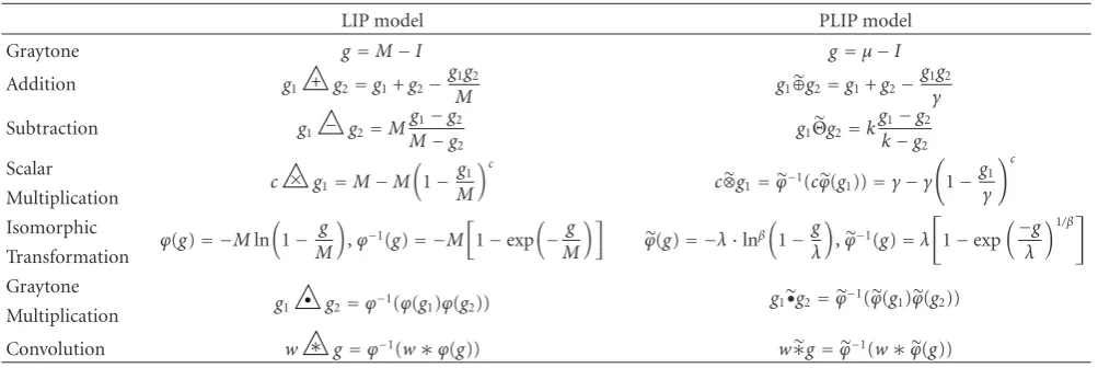
Table1: Summary of the LIP and PLIP model mathematical operators.

LIP model PLIP model

Graytone g=M−I g=μ−I

Addition g1 g2=g1+g2−

g1g2

M g1⊕g2=g1+g2−

g1g2

γ

Subtraction g1 g2=M

g1−g2

M−g2

g1Θg2=k

g1−g2

k−g2 Scalar

c g1=M−M

1−g1

M c

c⊗g1=ϕ−1(cϕ(g1))=γ−γ

1−g1

γ c

Multiplication Isomorphic

ϕ(g)= −Mln

1−_Mg

,ϕ−1_{(g)= −M}

1−exp

−_Mg

ϕ(g)= −λ·lnβ

1−g_λ

,ϕ−1_{(g)=λ 1−exp}

_−g

λ 1/β

Transformation Graytone

g1 g2=ϕ−1(ϕ(g1)ϕ(g2)) g1•g2=ϕ

−1_(ϕ(g 1)ϕ(g2)) Multiplication

Convolution w g=ϕ−1_{(w∗ϕ(g)) w∗g=ϕ}−1_(w∗ϕ(g))

2. Parameterized Logarithmic Image Processing

In this section, the PLIP model is reviewed. The model extends the concept of nonlinear image processing frame-works initially proposed by Jourlin and Pinoli [17] in the form of the LIP model. The advantageous properties of the added parameterization relative to the LIP model are analyzed.

The PLIP model generalizes the LIP model, which processes images as absorption filters known as graytones based on M, the maximum value of the range of I. The original LIP model is characterized by its isomorphic transformation, which mathematically emulates the relevant nonlinear physical model which the LIP model is based on. A new set of LIP mathematical operators, namely, addition, subtraction, and scalar multiplication, are consequently defined for graytones g₁ and g₂ and scalar constant c in terms of this isomorphic transformation, thus replacing traditional mathematical operators with nonlinear operators which attempt to characterize the nonlinearity of image arithmetic. For example, LIP addition emulates the intensity image projected onto a screen when a uniform light source is filtered by two graytones placed in series. Subsequently, LIP convolution is also defined for a graytonegand filterw [26].

Table 1 summarizes and compares the LIP and PLIP mathematical operators. In its most general form, the PLIP model generalizes graytone calculation, arithmetic opera-tions, and the isomorphic transformation independently, giving rise to the model parameters μ, γ, k, λ, and β. To reduce the number of parameters needed for image fusion, this paper considers the specific instance in which μ =

M, γ = k = λ, and β = 1, effectively resulting in a single model parameter γ. In this case, The PLIP model generalizes the isomorphic transformation which defines the LIP model by accordingly choosing values forγ. Practically, for images in [0,M), the value of γ can either be chosen such thatγ ≥ Mfor positiveγor can take on any negative value. The resulting PLIP mathematical operators based on the parameterized isomorphic transformation can be subsequently derived.

2.1. Properties. The PLIP properties to be discussed refer to the specific instance of the PLIP model in whichμ=M,γ=

k=λ, andβ=1. Similar intuitions are deduced for the more general cases.

1. The PLIP model operators revert to the LIP model operators withγ=M.

2. It can be shown that

lim

|γ|→ ∞ϕ(a) =|γlim|→ ∞ϕ

−1_{(a)=a. (1)}

Sinceϕandϕ−1_{are continuous functions, the PLIP} model operators revert to arithmetic operators as|γ|

approaches infinity, and therefore, the PLIP model approaches standard linear processing of graytone functions as|γ|approaches infinity. Depending on the nature of the algorithm, an algorithm which utilizes standard linear processing operators can be found to be an instance of an algorithm using the PLIP model withγ= ∞.

3. The PLIP model can generate intermediate cases between LIP operators and standard operators by choosingγin the range (M,∞).

4. For input graytones in [0,M), the range of PLIP addition and multiplication withγin [M,∞] is [0,γ]. 5. For input graytones in [0,M), the range of PLIP

subtraction withγin [M,∞] is (−∞,γ].

6. It can be shown that the PLIP operators obey the associative, commutative, and distributive laws and unit identities.

The 5th requirement essentially states that when visually “good” images are processed, the output must also be visually “good” [22]. The PLIP model satisfies the requirements by selecting values of γ which expands the dynamic range of outputs in order to minimize information loss while also retaining nonlinear, logarithmic functionality according to a physical model. Thus, for positive γ, the PLIP model physically provides a balance between the standard linear processing model and the LIP model. Conversely, negative values of γ may be selected for cases in which added brightness is needed to yield more visually pleasing results.

3. Parameterized Logarithmic Multiresolution

Image Decomposition Schemes

Image fusion algorithms using the PLIP model require a mathematical formulation of multiresolution decomposi-tion schemes and fusion rules in terms of the model. In this section, we introduce new parameterized logarithmic multiresolution decomposition schemes and fusion rules. It should be noted that they are defined for graytones. Therefore, images are converted to graytones before PLIP-based operations are performed and converted from gray-tone values to grayscale values after PLIP-based operations are performed.

3.1. Parameterized Logarithmic Laplacian Pyramid. The LP, originally proposed by Burt and Adelson [14], uses the Gaussian Pyramid to provide a multiresolution image repre-sentation for an imageI. Each analysis stage consists of low-pass filtering, downsampling, interpolating, and differencing steps in order to generate the approximation coefficients y(0n)and detail coefficients y(1n)at scale n. According to the PLIP model, the approximation coefficients for the Parameterized Logarithmic Laplacian Pyramid (PL-LP) of a graytonegat a scalen >0 are generated by

y0(n)=

w∗y0(n−1)

↓2, (2)

wherey(0n)= g,∗ denotes PLIP convolution, andwis a 2D lowpass filter. For example,wcan be defined by

w= 1

256 ⎡ ⎢ ⎢ ⎢ ⎢ ⎢ ⎢ ⎢ ⎢ ⎢ ⎣

1 4 6 4 1

4 16 24 16 4

6 24 36 24 6

4 16 24 16 4

1 4 6 4 1

⎤ ⎥ ⎥ ⎥ ⎥ ⎥ ⎥ ⎥ ⎥ ⎥ ⎦ . (3)

The detail coefficients at scalenare consequently calculated as a weighted difference between successive levels of the Gaussian Pyramid and are given by

y1(n)=y(

n)

0 Θ(4w)∗

y(0n+1)

↑2. (4)

The inverse procedure begins from the approximation coefficient at the high decomposition levelN. Each synthesis level reconstructs approximation coefficients at a scalei < N by each synthesis level by

y0(n)=y

(n)

1 ⊕(4w)∗

y0(n+1)

↑2. (5)

3.2. Parameterized Logarithmic Discrete Wavelet Transform.

The 2D separable DWT uses a quadrature mirror set of 1D analysis filters, g and h, and synthesis filters, gandh, to provide a multiresolution scheme for an image I with added directionality relative to the LP [15]. The DWT is able to provide perfect reconstruction while using critical sampling. Each analysis stage consists of filtering along rows, downsampling along columns, filtering along columns, and downsampling along rows in order to generate the approximation coefficient subbandy0(n)and detail coefficient subbandsy(1n),y(

n) 2 , andy(

n)

3 oriented horizontally, vertically, and diagonally, respectively, at scale n. The synthesis pro-cedure begins from the wavelet coefficients at the highest decomposition levelN. Filtering and upsampling steps are performed in order to perfectly reconstruct the image signal. According to the PLIP model, the Parameterized Logarithmic Discrete Wavelet Transform (PL-DWT) at graytone g at a decomposition leveln >0 is calculated by making use of the parameterized isomorphic transformation and is defined by

WDWT

y(0n)

=ϕ−1WDWT

ϕy0(n)

, (6)

where y(0)0 = g. Similarly, each synthesis level reconstructs approximation coefficients at a scalei < Nby

W−1

DWT WDWT y0(n)

=ϕ−1_W−1 DWT

ϕWDWT

y0(n)

. (7)

3.3. Parameterized Logarithmic Stationary Wavelet Transform.

Both the DWT and LP are shift-variant due to the down-sampling step which they employ. Therefore, the alteration of transform coefficients may introduce artifacts when processed using the DWT and to a lesser extent, the LP. It can introduce artifacts into the fusion results particularly for cases in which source images are misregistered. The SWT is a shift-invariant, redundant wavelet transform which attempts to reduce artifact effects by upsampling analysis filters rather than downsampling approximation images at each level of decomposition [27]. According to the PLIP model, the forward and inverse Parameterized Logarithmic Stationary Wavelet Transform (PL-SWT) for a graytonegat a decomposition leveln >0 is calculated by

WSWT

y(0n)

=ϕ−1_W SWT

ϕy0(n)

,

WSWT−1

WSWT

y0(n)

=ϕ−1WSWT−1

ϕWSWT

y(0n)

y(0n) φ W φ−1 φ−1 φ−1 φ−1

y0(n+1)

y1(n+1) y2(n+1)

y3(n+1)

φ

φ φ φ

W−1 _φ−1 _y(n) 0

Figure1: Parameterized Logarithmic Wavelet Transform analysis and synthesis.

(a) (b) (c)

(d) (e) (f)

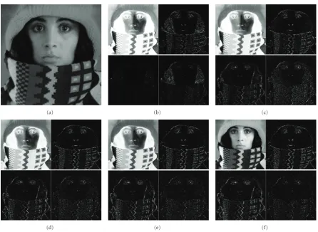
Figure2: (a) Original “Trui” image, top-left: approximation subband, magnitude of top-right: horizontal subband, bottom-left: vertical subband, bottom-right: diagonal subband magnitude of horizontal subband using the SWT and PLIP model operators with (b)γ=256 (LIP model case), (c)γ=300, (d)γ=500, (e)γ=700, and (f) standard mathematical operators.

Figure 1illustrates the analysis and synthesis stages using PLIP wavelet transforms, where W is a type of wavelet transform (e.g., DWT, SWT, etc.) with a given set of wavelet filters [28]. As the parameterized logarithmic decomposition approaches essentially make use of standard decomposition schemes with added preprocessing and postprocessing in the form of the isomorphic transformation calculations, they can be computed with minimal added computation cost.

Figure 2illustrates the advantages yielded using param-eterized logarithmic multiresolution schemes. The wavelet decomposition using γ = 256 (LIP model case) predom-inantly extracts the hair features from the image. As γ increases, it is particularly apparent that the hair textures are less emphasized and that the scarf, hat, and facial edges and textures are more emphasized. The wavelet decomposition using standard operators extracts the most texture and edge

information from the scarf, hat, and face in the image, and close to none of the texture of the hair. Visually, it is seen that the wavelet decomposition using the PLIP model operators withγ = 300 provides the best balance between extracting the hair, scarf, hat, and facial features in the image. Ultimately, the salient features which need to be extracted at each scale for further processing are task and image dependent, and thus, the PLIP model parameter can be tuned accordingly.

4. Image Fusion Using the PLIP Model

Image 1

Image 2

T

T Analysis

Pixel-based fusion rule

Pixel-based detail coefficient fusion rule Approximation coefficient fusion

rule

T1 Synthesis

Fused image

Figure3: A generalized pixel-based multiresolution image fusion algorithm.

and detail coefficient fusion rules according to the PLIP model. The combination of the parameterized logarithmic image decomposition techniques and fusion rules yields a new set of image fusion algorithms which are based on the PLIP model. Consequently, due to the generalization of the PLIP operators, image fusion algorithms using LIP operators and standard operators are also encapsulated by the proposed approaches.

4.1. Parameterized Logarithmic Pixel-Based Image Fusion.

A generalized pixel-based multiresolution image fusion algorithm is illustrated inFigure 3. The input source images are transformed using a given multiresolution image decom-position technique T. One fusion rule is used to fuse the approximation coefficients at the highest decomposition level. A second fusion rule is used to fuse the detail coef-ficients at each decomposition level. The resulting inverse transform yields the final fused result. Although image fusion algorithms are expected to withstand minor registration differences, the source images to be fused are assumed to be registered. Misregistered source images should be subjected to registration preprocessing steps independent to the image fusion algorithm. The approximation coefficients at the highest level of decompositionNare most commonly fused via uniform averaging. This is because at the highest level of decomposition, the approximation coefficients are interpreted as the mean intensity value of the source images with all salient features encapsulated by the detail coefficient subbands at their various scales [1]. Therefore, fusing approximation coefficients at their highest level of decomposition by averaging maintains the appropriate mean intensity needed for the fusion result with minimal loss of salient features. Given y(I1N,0)and y

(N)

I2,0, the approximation coefficient subbands of images I1 and I2, respectively, at the highest decomposition level N yielded using a given parameterized logarithmic multiresolution decomposition technique, the approximation coefficients for the fused imageFat the highest level of decomposition using simple averaging according to the PLIP model by

y(FN,0)=

1 2⊗

yI(1N,0)⊕y

(N) I2,0

. (9)

In general, an approximation coefficient fusion rule can be

adapted according to the PLIP model by

yF(N,0)=ϕ−1

RAϕyI(1N,0)

,ϕyI(N2,0)

, (10)

whereRAis an approximation coefficient fusion rule imple-mented using standard arithmetic operators. An analysis of the PLIP addition operation inTable 1and (9) yields a simple interpretation of the effect ofγon fusion results. Practically,γ can be interpreted as a brightness parameter, where negative values ofγyield brighter fusion results and positive values ofγ yield darker fusion results. This is achieved while also maintaining the fusion identity that the fusion of identical source images is the source image itself. Therefore, improved visual quality is achieved within an image fusion context and not as a result of an independent image enhancement process. The influence of the parameterization on fusion results is not limited to this na¨ıve observation, however, as the model parameter γ also influences the multiscale decomposition scheme and the detail coefficient fusion rule. Conversely, the detail coefficients of the source images correspond to salient features such as lines and edges detected at various scales. Therefore, fusion rules for detail coefficients at each decomposition level should be formu-lated in order to preserve these features. Such fusion rules are inspired by the human visual system, which is particularly sensitive to edges. Many pixel-based detail coefficient fusion rules have been proposed. In this paper, the absolute maximum (AM) and Burt and Kolczynski (BK) pixel-based detail coefficient fusion rules are considered and formulated according to the PLIP model. The parameterized logarithmic detail coefficient fusion rules are defined according to the PLIP model by

yF(n,i)=ϕ−1

RDϕyI(1n,)i

,ϕyI(2n,)i

, (11)

where RD is a coefficient fusion rule implemented using standard arithmetic operators.

4.1.1. Parameterized Logarithmic Absolute Maximum Detail Coefficient Fusion Rule. The AM detail coefficient fusion

each level of decompositionn, the multiplicative weights for fusion are given by

λ(in)(k,l)= ⎧ ⎪ ⎪ ⎨ ⎪ ⎪ ⎩

1, y(I1n,)i(k,l)

>y(I2n,)i(k,l) ,

0, y(I1n,)i(k,l)

≤yI(2n,)i(k,l) .

(12)

For each of the i highpass subbands at each level of decompositionn, the detail coefficients of the fused image Fare determined by

yF(n,i)(k,l)=λi(n)(k,l)y(I1n,)i(k,l) +

1−λ(in)(k,l)

y(I2n,)i(k,l). (13)

Accordingly, the parameterized logarithmic AM rule is yielded by (11).

4.2. Parameterized Logarithmic Burt and Kolczynski Detail Coefficient Fusion Rule. The BK detail coefficient fusion rule

combines detail coefficients based on an activity measure and a match measure [29]. The activity measure for eachw×w local window of each subbandiis calculated for each source image, given as

a(In,i)(k,l)=

(Δk,Δl)∈W

yI(n,i)(k+Δk,l+Δl) 2

. (14)

The local match measure of each subband measures the correlation of each subband between source images and is given as

m(I1n,)I2,i(k,l)

=2

(Δk,Δl)∈W

yI(1n,)i(k+Δk,l+Δl)

yI(2n,)i(k+Δk,l+Δl)

a(In1,)i(k,l) +a (n) I2,i(k,l)

.

(15)

Comparing the match measure to a thresholdthdetermines if detail coefficients are to be combined by simple selection or by weighted averaging. The associated weights for fusion are given by

λ(in)(k,l)= ⎧ ⎪ ⎪ ⎪ ⎪ ⎪ ⎪ ⎪ ⎪ ⎪ ⎪ ⎪ ⎪ ⎪ ⎪ ⎪ ⎪ ⎪ ⎪ ⎪ ⎪ ⎪ ⎪ ⎪ ⎪ ⎪ ⎪ ⎪ ⎪ ⎪ ⎪ ⎪ ⎪ ⎨ ⎪ ⎪ ⎪ ⎪ ⎪ ⎪ ⎪ ⎪ ⎪ ⎪ ⎪ ⎪ ⎪ ⎪ ⎪ ⎪ ⎪ ⎪ ⎪ ⎪ ⎪ ⎪ ⎪ ⎪ ⎪ ⎪ ⎪ ⎪ ⎪ ⎪ ⎪ ⎪ ⎩

1, m(In1,)I2,i(k,l)≤th, a(I1n,)i(k,l)> a

(n) I2,i(k,l),

0, m(In1,)I2,i(k,l)≤th, a(I1n,)i(k,l)≤a

(n) I2,i(k,l),

1 2+

1 2 ⎛

⎝1−m(I1n,)I2,i(k,l) 1−T

⎞ ⎠_{, m}(n)

I1,I2,i(k,l)> th,

a(I1n,)i(k,l)> a (n) I2,i(k,l),

1 2−

1 2 ⎛

⎝1−m(In1,)I2,i(k,l) 1−T

⎞ ⎠_{, m}(n)

I1,I2,i(k,l)> th,

a(I1n,)i(k,l)≤a (n) I2,i(k,l).

(16)

For each of the i highpass subbands at each level of decompositionn, the detail coefficients for the fused imageF are again determined by (13). Accordingly, the parameterized logarithmic BK rule is yielded by (11).

Figure 4illustrates the fundamental themes which have been discussed so far, particularly highlighting the necessity for the added model parameterization. The QW quality metric [25] included in Figure 4, whose details are to be discussed further in Section 5, implies a better fusion for a higher value of QW. Figure 4(c) shows that firstly, the PLIP model reverts to the LIP model with γ = M =

256, and secondly, that the combination of source images using this extreme case may still be visually unsatisfactory given the nature of the input images, even though the processing framework is based on a physically inspired model. Figures 4(d), 4(e), and 4(f) illustrate the way in which fusion results are affected by the parameterization, with the most improved fusion performance yielded by the proposed approach using parameterized multiresolution decomposition schemes and fusion rules relative to both the standard processing extreme and the LIP model extreme with γ=430. Namely, this result using the proposed approach has better visual contrast between roads and terrain and provides the proper base luminance to effectively differentiate between the grass and bushes.Figure 5plots theQW quality metric [25] as a function ofγand reflects the qualitative observation indicating Figure 4(e) as the best fusion output. Lastly, Figures4(g)and4(h)show using the AM fusion rule that the PLIP operators revert to standard mathematical operators as γapproaches infinity.

4.3. Parameterized Logarithmic Region-Based Image Fusion.

(a) (b) (c) (d)

(e) (f) (g) (h)

Figure4: (a) and (b) Original “navigation” source images, image fusion results using the LP/AM fusion rule, and PLIP model operators with (c)γ=256 (LIP model case),QW=0.3467, (d)γ=300,QW=0.7802, (e)γ=430,QW=0.8200, (f)γ=700,QW=0.8128 (g)γ=108, QW=0.7947, and (h) standard mathematical operators,QW=0.7947.

0.35 0.4 0.45 0.5 0.55 0.6 0.65 0.7 0.75 0.8 0.85

QW

200 400 600 800 1000 1200 1400

γ

Figure5: Plot ofQWversusγfor image fusion results inFigure 4,

indicating a maximum atγ=430,QW=0.8200.

The choice of segmentation algorithm used in region-based image fusion directly affects the fusion result. Seg-mentation algorithms which have been used in region-based image fusion algorithms include watershed [30], K-means [31], texture-based [32], pyramidal linking [1], and mean-shift segmentation [33]. In this paper, mean-shift segmentation is used for all region-based approaches because of its robustness [34,35]. It may be substituted with another segmentation algorithm. As this paper is primarily

concerned with the use of the nonlinear frameworks and multiresolution schemes for image fusion, a discussion of appropriate segmentation algorithms for image fusion is considered outside of the scope of this work. The main objective here is to extend the use of parameterized logarithmic image fusion to region-based approaches. A shared region representation for region-based image fusion purposes is yielded using mean-shift segmentation by indi-vidually segmenting each of the source images, and by then splitting overlapping regions into new regions [32]. An example of a shared region representation yielded using mean-shift segmentation is shown inFigure 7. To maintain consistency in segmentation results across different scales, successive downsampling is performed to yield a shared region representation at each level of decomposition based on the image decomposition scheme used for image fusion [33].

4.3.1. Region-Based Detail Coefficient Fusion Rules. Most any fusion rule formulated for pixel-based fusion can be easily formulated in terms of regions. The extension to regions merely involves calculating activity measures, match measures, and fusion weights for each region R instead of each pixel [1]. For experimental purposes, the activity measure for each region of each subband iof each source image is calculated by

a(In,i)(R)=

(k,l)∈R

y(In,i)(k,l) 2

Image 1

Image 2

T

Segmentation T Analysis and segmentation

Region-based fusion rule

Region-based detail coefficient

fusion rule Approximation coefficient fusion

rule

T1 Synthesis

Fused image

Figure6: A generalized region-based multiresolution image fusion algorithm.

(a) (b) (c) (d) (e)

Figure7: (a) and (b) Original “brain” source images, (c) mean-shift segmentation result of (a), (d) mean-shift segmentation result of (b), (e) shared region representation for region-based image fusion.

(a) (b)

(c) (d)

Figure 8: (a) and (b) Original “clock” source images, respective weights (c)c·λand (d)c·(1−λ) used for image fusion quality assessment.

where|R| is the area of the regionR. Similarly, the match measure m(I1n,)I2,i(R) and the multiplicative fusion weight λ(in)(R) for each region of each subband i can be defined

based on the fusion rule of choice. For experimental purposes, fusion weights are defined according to a region-based absolute maximum selection rule, hereby referred to as RB, by

λ(in)(R)= ⎧ ⎪ ⎪ ⎨ ⎪ ⎪ ⎩

1, a(In1,)i(R)

>a(In2,)i(R) ,

0, a(In1,)i(R)

≤a(In2,)i(R) .

(18)

For each of the i highpass subbands at each level of decompositionn, the detail coefficients of the fused image Fin each regionRare determined by

yF(n,i)(R)=λ (n) i (R)y

(n) I1,i(R) +

1−λ(in)(R)

yI(n2,)i(R). (19)

The parameterized logarithmic region-based image fusion rule is defined according to the PLIP model by (11).

5. Quantitative Image Fusion

Quality Assessment

(a) (b) (c) (d) (e)

(f) (g) (h) (i) (j)

(k) (l) (m) (n) (o)

(p) (q) (r) (s) (t)

Figure9: Zoomed regions of (a)and (b) Original “clock” source images, image fusion results using (c) LP and RB, (d) LIP-LP and RB, (e) PL-LP and RB, (f) and (g) original “brain” source images, image fusion results using (h) SWT and RB, (i) LIP-SWT and RB, (j) PL-SWT and RB(k) and (l) original “navigation” source images, image fusion results using (m) DWT and AM, (n) LIP-DWT and AM, (o) PL-DWT and AM(p) and (q) original “remote sensing” source images, image fusion results using (r) SWT and BK, (s) LIP-SWT and BK, (t) PL-SWT and BK.

such as region-based and even simple averaging approaches [25]. Nonetheless, to gain objective perspective not on the fusion rule or standard decomposition scheme of choice, but rather the improvement of fusion results using the PLIP model, fusion results are assessed quantitatively using the Piella and Heijmans image fusion quality metric. The metric measures fusion quality based on how much the fusion result reflects the original source images. Bovik’s quality index [38] is used to relate the fused result to its original source images. The quality index Q0 proposed by Bovik to measure the

similarity between two sequencesxandyis given by

Q0= σxy σxσy·

2μxμy μx2_+μy2·

2σxσy

σx2_+σy2, (20)

(a) (b) (c) (d) (e)

(f) (g) (h) (i) (j) (k)

(l) (m) (n) (o) (p) (q)

(r) (s) (t) (u) (v) (w)

(x) (y) (z) (aa) (bb) (cc)

Figure10: (a) and (b) Original “clock” source images, image fusion results using (c) LP/AM, (d) LIP-LP/AM, (e) PL-LP/AM, (f) LP/BK, (g) LIP-LP/BK, (h) PL-LP/BK, (i) LP/RB, (j) LIP-LP/RB, (k) PL-LP/RB, (l) DWT/AM, (m) LIP-DWT/AM, (n) PL-DWT/AM, (o) DWT/BK, (p) LIP-DWT/BK, (q) PL-DWT/BK, (r) DWT/RB, (s) LIP-DWT/RB, (t) PL-DWT/RB, (u) SWT/AM, (v) LIP-SWT/AM, (w) PL-SWT/AM, (x) SWT/BK, (y) LIP-SWT/BK, (z) PL-SWT /BK, (aa) SWT/RB, (bb) LIP-SWT/RB, (cc) PL-SWT/RB.

w×wwindow. The average of these quality indexes is used to measure the similarity betweenIandF, and is given by

Q0(I,F)= 1

|W|

w∈W

Q0(I,F|w). (21)

The resulting similarity index ranges from 0 to 1, with two identical images yielding aQ0equal to 1. Definings(I|w) as the saliency, and in this case, the variance of the imageIin a local windoww×wwindow, the quality of the fused result can be assessed by first calculating local weightsλ(w) for the source imagesI1andI2, given by

λ(w)= s(I1|w) s(I1|w) +s(I2|w)

(22)

and then calculating the fusion quality indexQ(I1,I2,F) for the fused resultFby

Q(I1,I2,F)

=_|1

W|

w∈W

(λ(w)Q0(I1,F|w) + (1−λ(w))Q0(I2,F|w)). (23)

(a) (b) (c) (d) (e)

(f) (g) (h) (i) (j) (k)

(l) (m) (n) (o) (p) (q)

(r) (s) (t) (u) (v) (w)

(x) (y) (z) (aa) (bb) (cc)

Figure11: (a) and (b) Original “brain” source images, image fusion results using (c) LP/AM, (d) LIP-LP/AM, (e) PL-LP/AM, (f) LP/BK, (g) LIP-LP/BK, (h) PL-LP/BK, (i) LP/RB, (j) LIP-LP/RB, (k) PL-LP/RB, (l) DWT/AM, (m) LIP-DWT/AM, (n) PL-DWT/AM, (o) DWT/BK, (p) LIP-DWT/BK, (q) PL-DWT/BK, (r) DWT/RB, (s) LIP-DWT/RB, (t) PL-DWT/RB, (u) SWT/AM, (v) LIP-SWT/AM, (w) PL-SWT/AM, (x) SWT/BK, (y) LIP-SWT/BK, (z) PL-SWT /BK, (aa) SWT/RB, (bb) LIP-SWT/RB, (cc) PL-SWT/RB.

regions in which the saliency of the source images is greater. Defining the overall saliency of a windowC(w) by

C(w)=max(s(I1|w),s(I2|w)). (24)

The weighted fusion quality indexQW(I1,I2,F) [25] is given by

Qw(I1,I2,F)

=

w∈W

c(w)(λ(w)Q0(I1,F|w) + (1−λ(w))Q0(I2,F|w)), (25)

where

c(w)= C(w)

w_∈WC(w) (26)

AsQ0yields a maximum value of 1 for identical input images, higher fusion quality metric values indicate better fusion results. Figure 8provides a graphical representation of the weights which are calculated by the quality metric in order to assess the quality of image fusion results.

6. Experimental Results

(a) (b) (c) (d) (e)

(f) (g) (h) (i) (j) (k)

(l) (m) (n) (o) (p) (q)

(r) (s) (t) (u) (v) (w)

(x) (y) (z) (aa) (bb) (cc)

Figure12: (a) and (b) Original “navigation” source images, image fusion results using (c) LP/AM, (d) LIP-LP/AM, (e) PL-LP/AM, (f) LP/BK, (g) LIP-LP/BK, (h) PL-LP/BK, (i) LP/RB, (j) LIP-LP/RB, (k) PL-LP/RB, (l) DWT/AM, (m) LIP-DWT/AM, (n) PL-DWT/AM, (o) DWT/BK, (p) LIP-DWT/BK, (q) PL-DWT/BK, (r) DWT/RB, (s) LIP-DWT/RB, (t) PL-DWT/RB, (u) SWT/AM, (v) LIP-SWT/AM, (w) PL-SWT/AM, (x) SWT/BK, (y) LIP-SWT/BK, (z) PL-SWT /BK, (aa) SWT/RB, (bb) LIP-SWT/RB, (cc) PL-SWT/RB.

for these experiments: (1) the extreme case in which the PLIP model operators yield the LIP model operators (γ = M), (2) standard operators, which are the extreme case of PLIP model operators withγ = ∞, (3) the case in whichγtakes on a value other thanMor∞. For easy reference, we refer to these cases as the LIP model operator case, standard operator case, and PLIP model operator case, respectively, though in reality, all are cases of the proposed PLIP-based approach. It should be noted that image fusion algorithms employing LIP-based multiresolution image decomposition schemes and fusion rules have not even been introduced to our knowledge. Thus, we refer to the LP, DWT, and LIP-SWT image fusion algorithms as the image fusion algorithms which use PLIP operators with γ = M to implement the fusion rules and LP, DWT, and SWT, respectively.

(a) (b) (c) (d) (e)

(f) (g) (h) (i) (j) (k)

(l) (m) (n) (o) (p) (q)

(r) (s) (t) (u) (v) (w)

(x) (y) (z) (aa) (bb) (cc)

Figure13: (a) and (b) Original “remote sensing” source images, image fusion results using (c) LP/AM, (d) LIP-LP/AM, (e) PL-LP/AM, (f) LP/BK, (g) LIP-LP/BK, (h) PL-LP/BK, (i) LP/RB, (j) LIP-LP/RB, (k) PL-LP/RB, (l) DWT/AM, (m) LIP-DWT/AM, (n) PL- DWT/AM, (o) DWT/BK, (p) LIP-DWT/BK, (q) PL-DWT/BK, (r) DWT/RB, (s) LIP-DWT/RB, (t) PL-DWT/RB, (u) SWT/AM, (v) LIP-SWT/AM, (w) PL-SWT/AM, (x) SWT/BK, (y) LIP-SWT/BK, (z) PL-SWT /BK, (aa) SWT/RB, (bb) LIP-SWT/RB, (cc) PL-SWT/RB.

emphasizes the transform which is used while keeping all other factors constant. In these experimental results,N =

3 for all methods, and both the pixel- and region-based fusion rules are examined. For the wavelet-based approaches, biorthogonal 2.2 filters are used. The fusion results are compared quantitatively by first normalizing source images and fused results to the range 0–255, and then using the Piella and Heijmans image fusion quality metricQW withw =7. This metric is used to determine the optimal parameter value forγ, with the resulting fused image thereby taken to be the result for a given parameterized logarithmic image fusion algorithm. This demonstrates the ability to tune the PLIP

model parameter in order to optimize results according to any metric used for quality assessment.

Table2: Quantitative quality assessment of image fusion results using the Piella and Heijmans quality metric.

Decomposition scheme

Fusion rule

Clocks Brain Navigation Remote sensing

Standard LIP PLIP Standard LIP PLIP Standard LIP PLIP Standard LIP PLIP

LP

AM 0.8914 0.9168 0.9300 0.7753 0.5256 0.7760 0.7947 0.3467 0.8200 0.8383 0.7842 0.8404

BK 0.8851 0.9123 0.9250 0.7748 0.5349 0.7762 0.7933 0.3512 0.8196 0.8293 0.7627 0.8300

RB 0.8849 0.9114 0.9241 0.7572 0.5327 0.7576 0.8051 0.3505 0.8187 0.8113 0.7424 0.8120

DWT

AM 0.8750 0.8979 0.9002 0.7124 0.5296 0.7292 0.7363 0.6011 0.7607 0.7672 0.7128 0.7695

BK 0.8745 0.8891 0.8918 0.6701 0.4886 0.6886 0.7333 0.6064 0.7600 0.7378 0.6770 0.7385

RB 0.8763 0.8955 0.8972 0.6872 0.5008 0.7060 0.7288 0.6052 0.7589 0.7162 0.6869 0.7170

SWT

AM 0.8879 0.9085 0.9134 0.7539 0.5581 0.7718 0.7460 0.7250 0.7746 0.8137 0.7954 0.8150

BK 0.8926 0.9081 0.9130 0.7554 0.5714 0.7647 0.7382 0.7294 0.7821 0.8203 0.8045 0.8238

RB 0.8877 0.9045 0.9064 0.7458 0.5557 0.7684 0.7542 0.6873 0.7695 0.8078 0.7882 0.8080

The 2nd row shows that the proposed method is able to better capture the terrain information and road information of the respective source images. The 3rd row shows the improved contrast of tissue information and dense bone structure yielded by the proposed method. Lastly, the 4th row shows that the proposed fusion approaches are able to better capture the subtle features at the point at which the roads intersect. Thus, the experimental results highlight the improvement of fusion results yielded using the PLIP model operators. While the standard operator extreme can often give adequate results, the contrast and luminance can be improved by choosing a value ofγ which both reflects the human visual system and meets the dynamic range requirements of the input images. While the LIP model operator extreme can improve the performance of image fusion relative to standard operator extreme when the source images are similar in luminance (as in the case of the clocks images), it yields visually inadequate results for source images with greatly different local base luminance. This is particularly visible for input images in which one of the source images is predominantly dark as in the case of the “navigation” and “brain” images.

The quantitative observations are reflected by their corresponding quality metric values in Table 2, in which rows correspond to the basic multiresolution decomposition scheme and fusion rule employed and columns correspond to the image processing operators (LIP model operator case, standard operator case, or PLIP model operator case) used to implement the given decomposition scheme and fusion rule. It should be noted that a single, constant-size window is used in calculating the quality metric values. Thus, such an evaluation may be dependent on how well the window size reflects the scale of the objects of interest in the source images and may not be able to effectively quantify differences in fusion results even when qualitative visual differences are seen. This provides a rationalization as to why the perceived visual improvement of the proposed methods may in some cases only translate to a small increase in the quality metric values and continues to affirm the fact that objective image fusion quality assessment is still an open research topic. However, the rank of the scores is generally indicative of relative performance, and to standardize the

testing procedure and to maintain the same formulation of the metric as it was originally proposed, the same parameters are used to calculate quality metric values for all test cases. Thus, the quantitative analysis serves as an objective means of validating subjective observations. The quality metric values inTable 2show that, in all cases, fusion algorithms using the parameterized logarithmic multiresolution decomposition schemes and fusion rules outperform their respective general linear processing model counterparts.

7. Conclusions

Acknowledgments

This work has been partially supported by NSF Grant HRD-0932339. The authors would like to thank Dr. Oliver Rockinger for kindly providing the registered images used for computer simulations and to the anonymous referees for their invaluable suggestions which substantially improved the quality of this paper.

References

[1] G. Piella, “A general framework for multiresolution image fusion: from pixels to regions,”Information Fusion, vol. 4, no. 4, pp. 259–280, 2003.

[2] P. Hill, N. Canagarajah, and D. Bull, “Image fusion using complex wavelets,” inProceedings of the 13th British Machine Vision Conference, pp. 487–496, Cardiff, UK, 2002.

[3] M. Kumar and S. Dass, “A total variation-based algorithm for pixel-level image fusion,” IEEE Transactions on Image Processing, vol. 18, no. 9, pp. 2137–2143, 2009.

[4] S. Daneshvar and H. Ghassemian, “MRI and PET image fusion by combining IHS and retina-inspired models,”Information Fusion, vol. 11, no. 2, pp. 114–123, 2010.

[5] Y. Yang, D. S. Park, S. Huang, and N. Rao, “Medical image fusion via an effective wavelet-based approach,” EURASIP Journal on Advances in Signal Processing, vol. 2010, Article ID 579341, 13 pages, 2010.

[6] Z. Zhang and R. Blum, “Region-based image fusion scheme for concealed weapon detection,” inProceedings of the 31st Annual Conference on Information Sciences and Systems, pp. 168–173, 1997.

[7] X.-Q. Zhang, Z.-S. Gao, and H.-Z. Yuan, “Dynamic infrared and visible image sequence fusion based on DT-CWT using GGD,” in Proceedings of the International Conference on Computer Science and Information Technology (ICCSIT ’08), pp. 875–878, September 2008.

[8] Y. Chibani, “Selective synthetic aperture radar and panchro-matic image fusion by using the `a trous wavelet decomposi-tion,”EURASIP Journal on Applied Signal Processing, vol. 2005, no. 14, pp. 2207–2214, 2005.

[9] S.-Y. Zhang, P. Wang, X. Chen, and X. Zhang, “A new method for multi-source remote sensing image fusion,” in Proceedings of the IEEE International Geoscience and Remote Sensing Symposium (IGARSS ’05), pp. 3948–3951, July 2005. [10] Z. Zhang and R. S. Blum, “A categorization of

multiscale-decomposition-based image fusion schemes with a perfor-mance study for a digital camera application,”Proceedings of the IEEE, vol. 87, no. 8, pp. 1315–1326, 1999.

[11] P. S. Chavez Jr. and A. Y. Kwarteng, “Extracting spectral con-trast in Landsat Thematic Mapper image data using selective principal component analysis,”Photogrammetric Engineering & Remote Sensing, vol. 55, no. 3, pp. 339–348, 1989.

[12] T.-M. Tu, S.-C. Su, H.-C. Shyu, and P. S. Huang, “Efficient intensity-hue-saturation-based image fusion with saturation compensation,”Optical Engineering, vol. 40, no. 5, pp. 720– 728, 2001.

[13] M. Tabb and N. Ahuja, “Multiscale image segmentation by integrated edge and region detection,”IEEE Transactions on Image Processing, vol. 6, no. 5, pp. 642–655, 1997.

[14] P. J. Burt and E. H. Adelson, “Lapacian pyramid as a compact image code,”IEEE Transactions on Communications, vol. 31, no. 4, pp. 532–540, 1983.

[15] S. G. Mallat, “Theory for multiresolution signal decomposi-tion: the wavelet representation,”IEEE Transactions on Pattern Analysis and Machine Intelligence, vol. 11, no. 7, pp. 674–693, 1989.

[16] O. Rockinger, “Image sequence fusion using a shift-invariant wavelet transform,” inProceedings of the International Confer-ence on Image Processing, pp. 288–291, October 1997. [17] M. Jourlin and J. C. Pinoli, “Logarithmic image processing: the

mathematical and physical framework for the representation and processing of transmitted images,”Advances in Imaging and Electron Physics, vol. 115, pp. 126–196, 2001.

[18] J.-C. Pinoli, “A general comparative study of the multiplicative homomorphic, log-ratio and logarithmic image processing approaches,”Signal Processing, vol. 58, no. 1, pp. 11–45, 1997. [19] G. Deng, L. W. Cahill, and G. R. Tobin, “The study of logarithmic image processing model and its application to image enhancement,”IEEE Transaction on Image Processing, vol. 18, pp. 1135–1140, 2009.

[20] C. Vertan, A. Oprea, C. Florea, and L. Florea, “A pseudo-logarithmic image processing framework for edge detection,” inAdvanced Concepts for Intelligent Vision Systems, vol. 5259 ofLecture Notes in Computer Science, pp. 637–644, 2008. [21] J. Debayle, Y. Gavet, and J.-C. Pinoli, “General adaptive

neigh-borhood image restoration, enhancement and segmentation,” inProccedings of the International Conference on Image Analysis and Recognition (ICIAR ’06), vol. 4141 of Lecture Notes in Computer Science, pp. 29–40, Springer, Heidelberg, Germany, 2006.

[22] K. A. Panetta, E. J. Wharton, and S. S. Agaian, “Human visual system-based image enhancement and logarithmic contrast measure,”IEEE Transactions on Systems, Man, and Cybernetics, Part B, vol. 38, no. 1, pp. 174–188, 2008.

[23] E. J. Wharton, K. Panetta, and S. S. Agaian, “Logarithmic edge detection with applications,” inIEEE International Conference on Systems, Man, and Cybernetics (SMC ’07), pp. 3346–3351, October 2007.

[24] E. Wharton, S. Agaian, and K. Panetta, “Comparative study of logarithmic enhancement algorithms with performance measure,” inImage Processing: Algorithms and Systems, Neural Networks, and Machine Learning, vol. 6064 ofProceedings of the SPIE, p. 342353, San Jose, Calif, USA, 2006.

[25] G. Piella and H. Heijmans, “A new quality metric for image fusion,” inProceedings of International Conference on Image Processing (ICIP ’03), vol. 2, pp. 173–176, September 2003. [26] J. M. Palomares, J. Gonzalez, and E. Ros, “Designing a

fast convolution under the LIP paradigm applied to edge detection,” inProceedings of the 3rd International Conference on Advances in Pattern Recognition (ICAPR ’05), vol. 3687 of Lecture Notes in Computer Science, pp. 560–569, Bath, UK, August 2005.

[27] J. E. Fowler, “The redundant discrete wavelet transform and additive noise,”IEEE Signal Processing Letters, vol. 12, no. 9, pp. 629–632, 2005.

[28] G. Courbebaisse, F. Trunde, and M. Journlin, “Wavelet transform and LIP model,”Image Analysis and Stereology, vol. 21, no. 2, pp. 121–125, 2002.

[29] P. J. Burt and R. J. Kolczynski, “Enhanced image capture through fusion,” inProceedings of the 4th International Con-ference on Computer Vision, pp. 173–182, May 1993.

[31] A. M. Khan, B. Kayani, and A. M. Gillani, “Feature level fusion of night vision images based on K-means clustering algo-rithm,” inInnovations and Advanced Techniques in Computer and Information Sciences and Engineering, pp. 73–76, Springer, 2007.

[32] Z. Li, Z. Jing, G. Liu, S. Sun, and H. Leung, “A region-based image fusion algorithm using multiresolution segmentation,” inProceedings of the IEEE International Conference on Intelli-gent Transportation Systems, vol. 1, pp. 96–101, 2003. [33] L. Shuang and L. Zhilin, “A region-based technique for fusion

of high-resolutino images using mean shift segmentation,” in International Archives of the Photogrammetry, Remote Sensing, and Spatial Information Sciences, vol. 38, pp. 1267–1272, Beijing, China, 2008.

[34] D. Comaniciu and P. Meer, “Mean shift: a robust approach toward feature space analysis,”IEEE Transactions on Pattern Analysis and Machine Intelligence, vol. 24, no. 5, pp. 603–619, 2002.

[35] W. Tao, H. Jin, and Y. Zhang, “Color image segmentation based on mean shift and normalized cuts,”IEEE Transactions on Systems, Man, and Cybernetics, Part B, vol. 37, no. 5, pp. 1382–1389, 2007.

[36] C. S. Xydeas and V. Petrovi´c, “Objective image fusion perfor-mance measure,”Electronics Letters, vol. 36, no. 4, pp. 308–309, 2000.

[37] G. Qu, D. Zhang, and P. Yan, “Information measure for performance of image fusion,”Electronics Letters, vol. 38, no. 7, pp. 313–315, 2002.