Volume 2008, Article ID 264638,15pages doi:10.1155/2008/264638
Research Article
Localization Accuracy of Track-before-Detect Search Strategies
for Distributed Sensor Networks
Thomas A. Wettergren and Michael J. Walsh
Naval Undersea Warfare Center, 1176 Howell Street, Newport, RI 02841, USA
Correspondence should be addressed to Thomas A. Wettergren,[email protected]
Received 22 March 2007; Revised 29 June 2007; Accepted 30 August 2007
Recommended by Frank Ehlers
The localization accuracy of a track-before-detect search for a target moving across a distributed sensor field is examined in this paper. The localization accuracy of the search is defined in terms of the area of intersection of the spatial-temporal sensor coverage regions, as seen from the perspective of the target. The expected value and variance of this area are derived for sensors distributed randomly according to an arbitrary distribution function. These expressions provide an important design objective for use in the planning of distributed sensor fields. Several examples are provided that experimentally validate the analytical results.
Copyright © 2008 T. A. Wettergren and M. J. Walsh. This is an open access article distributed under the Creative Commons Attribution License, which permits unrestricted use, distribution, and reproduction in any medium, provided the original work is properly cited.
1. INTRODUCTION
Advances in miniaturization, electronics, and communica-tions have made the use of sensor networks a popular choice for providing surveillance coverage in diverse application ar-eas. Much of the current emphasis is on improved detection, classification, and localization of a single point in the surveil-lance region. However, recently, the use of a set of sensors that are geometrically distributed over a large area has been proposed as a cost-effective approach for tracking moving targets through surveillance regions (see, e.g., [1–3]). When designing these distributed sensor systems, the placement of the sensors within the field becomes a critical component of the design. Parametric representations of system perfor-mance goals, in terms of field parameters, provide an ability to appropriately consider trade-offs in the system design.
It has been shown by Cox [4] that beneficial detection performance can be obtained by sparsely distributed sensor networks when a multisensor detection strategy is employed in conjunction with a simple consistency check against ex-pected target kinematics (i.e., a track-before-detect search procedure). By exploiting this kinematic check, these meth-ods have been shown [5] to be robust against false alarms. This feature of track-before-detect strategies has been used to generate simple tracking procedures [6] that are robust against false alarms and require minimal between-sensor processing. The track-before-detect construct for distributed
sensor networks is based on the ability of the collabora-tive effort of fixed, but distributed, sensors to report detec-tions (over a network) to some higher-level system, where, then, a system-level detection decision is made based on a track estimate derived from the multiple detection reports. This higher-level system has the added benefit of effectively “weeding-out” false alarms that are inconsistent across the network; this benefit is one of the driving forces behind the employment of distributed sensor fields in harsh envi-ronments where communications capability between sensors is severely constrained. Other approaches to tracking tar-gets with simple kinematics using sensor networks revolve around either a search theory perspective [7] or computa-tionally efficient enumeration and filtering of potential tracks [8].
studies [10] have shown how probabilistic modeling of tar-get motion affects the efforts of a single searcher looking for the uncertain moving target. In this paper, we examine a re-lated aspect of the track-before-detect search strategy for dis-tributed sensor networks; namely, the localization accuracy of the search. Localization accuracy is defined in terms of the area of intersection of the sensor spatial-temporal coverage regions as seen from the target frame of reference. From this perspective, it is the target that is fixed, and the sensors that move with constant velocity (in the opposite direction). We show that, givenkdetections, the target is detected by a set ofksensors if and only if in the target coordinate system, the target is in the area of intersection of the coverage regions of these sensors. This area of intersection provides a measure (both graphical and quantifiable) of the expected area of un-certainty of the target location at a fixed point in time—even when the multiple sensor detections are not simultaneously obtained. The availability of a rapid assessment of expected localization accuracy in terms of sensor and target character-istics creates an invaluable design tool for proper positioning of sensors within the field.
This paper develops a set of calculations to determine the amount of expected localization accuracy that is attributable to the kinematic basis of track-before-detect methods. Un-der the assumption that individual sensor nodes report de-tections within some predictable range at a predictable accu-racy, we build a simple model of track-before-detect system-level performance for a generic distributed sensor network. While this performance is not meant to be representative of any particular sensor system, it illustrates the impact of tar-get kinematics on track-before-detect as a function of sensor positions.
The remainder of this paper is organized as follows. In Section 2, we describe sensor coverage in both sensor and tar-get coordinate systems, define the area of intersection of these coverage regions given k detections, and derive an expres-sion for this area in terms of sensor and target variables. We then compute the expected area of intersection, and the vari-ance of this area, for sensors distributed randomly according to a fixed and known, but arbitrary, distribution function. InSection 3, these results are used to calculate the expected value and variance of the area of intersection, given 1, 2, 3, or more detections on a target passing through the sensor field.Section 4includes examples that verify experimentally the analytical results of Sections2and3. These examples in-clude a uniformly distributed sensor field, a sensor “barrier” consisting of sensors distributed uniformly inxand normally in y, and, finally, an arbitrarily distributed sensor field. We conclude inSection 5with a summary of our findings, and some suggestions for further study.
2. INTERSECTION OF SENSOR SPATIAL-TEMPORAL COVERAGE REGIONS
We consider the problem of a set ofNfixed identical sensors deployed to search for a single moving target using a track-before-detect search strategy. We limit our exposition to the discussion of a single target; the extension to multiple targets is discussed in the conclusion. LetS⊆R2denote the region
Rd −
→x i
−→x j
V T
ΩT
θ
−→x T(t0)
− →x
T(t0+T)
Figure1: Detection regionΩTin sensor coordinate system. Sensors iandjare in the detection region.
to be searched over the time intervalt0≤t≤t0+T (hence-forth referred to as the search interval), and letxT(t) denote the location of the target at timet. We assume that the tar-get remains in the search regionSand moves with constant speedVin a fixed directionθthroughout the search interval. The target track over the search interval is then given by
xT
t=xT
t0
+t−t0
Vcosθ, sinθ, (1)
where we recall thattparameterizes the search intervalt0 ≤ t ≤t0+T. Letxi,i = 1,. . .,Ndenote the locations inSof Nfixed sensors. We assume the sensors all have identical fi-nite detection rangeRd and known probability of detection
Pd. A target detection is defined to occur on sensori dur-ing the search interval with probabilityPd if and only if the target passes within a distanceRdof the sensor (during that interval). Define the regionΩTas
ΩT=
x∈R2:x−x
T(t)≤Rd,t0≤t≤t0+T
, (2)
where·denotes Euclidean distance. Hence, if sensori de-tects the target during the search interval, then xi ∈ ΩT. Moreover, ifksensors detect the target during the search in-terval, thenxi1,. . .,xik ∈ ΩT for some subset{i1,. . .,ik}of
{1,. . .,N}. The regionΩT, referred to as a “target pill” in [9] because of its shape, is depicted inFigure 1. This region is the spatial-temporal coverage, or detection, region for the target. A natural measure of localization accuracy is the area of uncertainty, which identifies a region of the search spaceS
where the target is located. Often, the area of uncertainty is presented as a collection of closed sets, where each member of the collection identifies a region ofSwhere the target is lo-cated with a certain probability. The area of uncertainty pre-sented in this paper is a single connected closed subset ofS
that contains the target with a probability one.
Rd
Rd
V T
V T
Ωi
Ωj
θ
xi(t0)
xi(t0+T)
xj(t0)
xj(t0+T)
xT(t0)
Figure2: Detection regionsΩiandΩjin target coordinate system.
At timet0, the target locationxT(t0) is in the intersection of the
detection regions for sensorsiandj.
reference, the target is fixed and the sensors move with speed
Vin directionθ+π. The track of sensoriin the target coor-dinate system over the search interval is then given by
xi(t)=xi
t0
+t−t0
Vcos(θ+π), sin (θ+π)
=xi
t0
−t−t0
Vcosθ, sinθ.
(3)
Recall that in the sensor coordinate system, if sensoridetects the target during the search interval, then the target passes within a distanceRd of the sensor. Thus, in the target coor-dinate system, if the target is detected by sensoriduring the search interval, then the sensor passes withinRdof the target. Fori=1,. . .,N, let
Ωi=
x∈S:x−xi(t)≤Rd,t0≤t≤t0+T
(4)
represent the region of target detectability about sensor i. Thus, if sensoridetects the target during the search interval
t0≤t≤t0+T, thenxT(t0)∈Ωi. Furthermore, if the target is detected byksensors (e.g., sensorsi1,. . .,ik), then the target at timet0must lie in the intersection of the detection regions for these sensors, denotedΩint(k), that is,
xT
t0
∈
1≤j≤k
Ωij≡Ωint(k). (5)
This situation is depicted inFigure 2for the case where the target is detected by two sensors, labelediandj. The region of intersection of the two “pills”Ωi andΩj is the spatial-temporal detection region for the target in the target coor-dinate system.
LetAΩdenote the area of the detection regionΩT. Since
the transformation between the sensor and target reference frames is a pure translation, and since the sensor model is homogeneous in detection characteristics, it follows that
AΩ =area(Ωi) fori =1,. . .,N as well. Givenkdetections,
let Aint(k) denote the area of intersection of the k detec-tion regions in the target coordinates, that is, letAint(k) = area(Ωint(k)). From the example inFigure 2, it is clear that Aint(k) is a complicated function of the sensor locations, the sensor detection radius, the target initial location, course,
Rd
Rd
2Rd
V T
Ωi
(xi,yi)
Figure3: Rectangular coverage region for sensoriin target coordi-nates.
and speed, and the length of the search interval. However, for
V T Rd, the regionΩi, with areaAΩ =πR2d+ 2RdV T, is well approximated by the bounding rectangular region with dimensions 2Rd×(2Rd+V T), and with area 4R2d+ 2RdV T. Recall that all sensors translate identically under the transfor-mation to target coordinates, so all of the bounding rectan-gles for the different sensors are similarly aligned. Thus the intersection of any two of these overlapping rectangular de-tection regions is itself a rectangle with area greater than that of the intersection of the pills they bound. By induction, the intersection of anykof these overlapping rectangles,k ≥2, is a rectangle with area greater than that of the intersection of thekcorresponding pills. It follows that the area of inter-section for the rectangular approximation to the pill-shaped detection regions is strictly greater than the area of the actual intersection and, hence, provides a strict upper bound on the area of uncertainty for track-before-detect systems under the circular “cookie-cutter” sensor model under consideration.
Throughout the sequel, letΩi, the coverage region of sen-sor i in the target frame of reference, be the rectangle of lengthLy = 2Rd +V T and widthLx = 2Rd. The rectan-gles are oriented such that the longer axis is parallel to the direction of target motion, taken here to be, without loss of generality,θ=π/2, corresponding to they-axis. (Extensions to arbitrary target courseθ are obtained by a simple rota-tion of coordinate axes.) The coverage regionΩiis depicted inFigure 3. Note that the direction of sensor motion in the target coordinate system isθ+π=π/2 +π=3π/2. This ge-ometrical construction leads toΩi= {(x,y)∈S:xi−Rd ≤
x ≤ xi+Rd,yi−V T−Rd ≤ y ≤ yi+Rd}for any sensor
i∈ {1,. . .,N}that detects the target. With these definitions, the following lemma provides a formula for the area of inter-section of these rectangular detection regions in target coor-dinates givenkdetections.
Lemma 1. Suppose there arek≥1regionsΩiwith nonempty
i∈ {1,. . .,k}. Letdx(k)anddy(k)be defined as follows:
dx(k)=max 1≤i≤k
xi
−min 1≤i≤k
xi
,
dy(k)=max 1≤i≤k
yi
−min 1≤i≤k
yi
. (6)
ThenAint(k), the area of the region of joint intersectionΩint(k)
(as defined in(5)), is given by
Aint(k)=
Lx−dx(k)
Ly−dy(k)
. (7)
Proof. Take any point p =(u,v) inR2. Then p ∈Ω
int(k) if and only if
xi−Rd≤u≤xi+Rd,
yi−V T−Rd≤v≤yi+Rd,
(8)
fori=1,. . .,k. These inequalities hold if and only if
max 1≤i≤k
xi
−Rd≤u≤min 1≤i≤k
xi
+Rd,
max 1≤i≤k
yi
−V T−Rd≤v≤min 1≤i≤k
yi
+Rd.
(9)
Since the pointp=(u,v) inR2is arbitrary, it follows that
Ωint(k)=
max 1≤i≤k
xi
−Rd, min 1≤i≤k
xi
+Rd
×
max 1≤i≤k
yi
−V T−Rd, min 1≤i≤k
yi
+Rd . (10)
Now,
min 1≤i≤k
xi
+Rd−
max 1≤i≤k
xi
−Rd
=min 1≤i≤k
xi
−max 1≤i≤k
xi
+ 2Rd=Lx−dx(k).
(11)
Likewise,
min 1≤i≤k
yi
+Rd−
max 1≤i≤k
yi
−V T−Rd
=min 1≤i≤k
yi
−max 1≤i≤k
yi
+ 2Rd+V T=Ly−dy(k). (12)
Thus the areaAint(k) of the intersectionΩint(k) is equal to (Lx−dx(k))(Ly−dy(k)). Note that fork=1,dx(1)=dy(1)= 0, andAint(1)=LxLy=(2Rd)(2Rd+V T)=AΩ, as expected.
This lemma explicitly shows that the region of poten-tial target locations for k detections,Ωint(k), and its area, Aint(k), are functions of the sensor detection rangeRd, the sensor locationsx1,. . .,xk, the target speedV, and the length T of the search interval. Implicitly,Ωint(k) and Aint(k) are also functions of initial target locationxT(t0), as the partic-ulark-subset ofN sensors that detect the target obviously depends on the location of the target in the search spaceS. In general, any one of these variables may be random. This paper is concerned with the statistics ofAint(k) as a func-tion ofxT(t0) whenRd,V, andTare fixed and known, and the sensor locationsx1,. . .,xN are distributed randomly in
S according to a fixed and known, but arbitrary, distribu-tion funcdistribu-tion. The explicit computadistribu-tion of the expected value and variance ofAint(k) in terms ofRd,V,T,x1,. . .,xk, and
xT(t0) provides a means for representing localization accu-racy of track-before-detect search strategies in terms of these important distributed sensor system design parameters.
xi
xj
ΩT xT(t0+T)
xT(t0)
Ly
(xΩ,yΩ)
Lx
Figure4: Rectangular detection region in sensor coordinates.
2.1. Expected value ofAint(k)
Suppose there arek ≥ 1 detections on sensorsi =1,. . .,k. Since these sensors detect the target during the search inter-val, then it must be the case that, in the sensor frame of refer-ence,x1,. . .,xk ∈ΩT. This situation is depicted inFigure 4, where only sensors iand j, 1 ≤ i < j ≤ k, are explicitly labeled. Let x(1),. . .,x(k) and y(1),. . .,y(k) denote the order statistics [11] associated with thexandycoordinates, respec-tively, of theksensor locations. Lemma 1gives the area of intersectionAint(k) of the detection regionΩint(k) as a func-tion of the range (the maximum value minus the minimum value) of the order statistics x(1),. . .,x(k) and y(1),. . .,y(k), that is,dx(k)= x(k)−x(1)anddy(k)= y(k)−y(1). We use known results on the range of order statistics [11] to com-pute the expected value and variance of the area of intersec-tionAint(k).
FromLemma 1, the area of intersection of the detection regionsΩ1,. . .,Ωkis given by
Aint(k)=AΩ
1−dx(k)
Lx
1−dy(k)
Ly
, (13)
whereAΩ =LxLy is the area of the coverage regionΩiof a single sensor. If the sensor locations are distributed indepen-dently inxandy, then the expected value ofAint(k) is given by
EAint(k)
=AΩ
1−E
dx(k)
Lx
1−E
dy(k)
Ly
. (14)
The sensor locations within the search regionSare assumed to be random, with a fixed and known distribution function. LetF(x,y) represent the distribution function ing to the random locations of the sensors. The correspond-ing density function f(x,y) is given byf =F. Furthermore, let fXandfY represent the marginal density functions of the sensor locations in thexandycoordinates, respectively, with associated distribution functionsFXandFY. Since the ranges
theory of order statistics (see Stuart and Ord [11, page 495]), the expected value ofdx(k) is given by
Edx(k)=
xΩ+Lx
xΩ
1−FX|ΩT(x)
k
−1−FX|ΩT(x)
k
dx,
(15)
whereFX|ΩTandFY|ΩTrepresent the conditional distribution
functions forFXandFY, respectively, conditioned on the de-tection regionΩT. Equation (15) is derived in [11] by sub-stituting the well-known density functions for the minimum and maximum order statisticsx(1)andx(k)into the identity E(dx(k))=E(x(k))−E(x(1)), and using integration by parts to simplify the resulting expression. A similar expression to (15) holds for the expected value of the rangedy(k).
The conditional distribution functionFX|ΩTis given by
FX|ΩT(x)= ⎧ ⎪ ⎪ ⎪ ⎪ ⎨ ⎪ ⎪ ⎪ ⎪ ⎩
0, x < xΩ,
x
xΩ
fX|ΩT(ξ)dξ, xΩ≤x≤xΩ+Lx,
1, x > xΩ+Lx,
(16)
where the point (xΩ,yΩ) denotes the lower left-hand corner
ofΩT(seeFigure 4), and
fX|ΩT(x)=
fX(x)
xΩ+Lx
xΩ fX(ξ)dξ
, xΩ≤x≤xΩ+Lx, (17)
and similarly forFY|ΩTand fY|ΩT. Thus, for a known
distri-bution on the sensor locations, the expected value of the area of the target location region is computed from (14), (15), and (16) (including the corresponding expressions forE(dy(k)) andFY|ΩT(y)).
If the sensor locations are not distributed independently inxandy, the expectation operator does not, in general, dis-tribute across terms inAint(k) by (14). However, in practice, we expect long, narrow detection regions, which is the case forV T Rd. For a target with courseθ=π/2, this trans-lates to a detection regionΩTwithLyLx. Also, for a search regionSmuch larger than the detection regionΩT, we ex-pect the variation infX|ΩTover the intervalxΩ≤x≤xΩ+Lx
to be small for all values ofxΩ. With these assumptions, the
sensorxandylocations are distributed approximately inde-pendently inΩT, with sensorxlocation approximately uni-formly distributed in this region, yielding
fX|ΩT(x)= ⎧ ⎪ ⎪ ⎨ ⎪ ⎪ ⎩
1
Lx, xΩ≤x≤xΩ+Lx,
0, otherwise,
(18)
which greatly simplifies the evaluation of (15).
2.2. Variance ofAint(k)
The variance of the area of intersection of the detection re-gionsΩ1,. . .,Ωk, denoted var(Aint(k)), is given by
varAint(k)
=EAint(k)−E
Aint(k)
2
=EAint(k)
2
−EAint(k)
2
,
(19)
whereE(Aint(k)) is given by (14). As in the previous section, the sensorxandylocations are approximately independent (within the local regionΩT), leading to
EAint(k)
2
=A2
ΩE
1−dx(k)
Lx
2
E
1−dy(k)
Ly
2
,
(20)
where
E
1−dx(k)
Lx
2
=1−2E
dx(k)
Lx +E
d2
x(k)
L2 x
=1−2E
dx(k)
Lx +
Edx(k)2+ vardx(k)
L2 x
=
1−E
dx(k)
Lx
2
+var
dx(k)
L2 x
,
(21)
and similarly for thedy(k) term. The expected value of the rangedx(k) is given by (15); a similar expression gives the ex-pected value of the rangedy(k). The variances of the ranges
dx(k) and dy(k) are found using known results on order statistics. From [11, page 495],
vardx(k)
=2
xΩ+Lx
xΩ
x(n)
xΩ
1−FX|ΩT
x(n)
k
−1−FX|ΩT
x(1)
k
+FX|ΩT
x(n)
−FX|ΩT(x(1))
k
dx(1)dx(n)−(E(dx(k)))2
(22)
fork ≥1, and similarly for var(dy(k)). The change of vari-ablesu=x(k),v=(x(1)−xΩ)/(x(k)−xΩ) replaces the iterated
integral in (22) by one with constant limits of integration, yielding
vardx(k)
=2
xΩ+Lx
xΩ
1
0
1−FX|ΩT(u)
k
−1−Fx|ΩT
(1−v)xΩ+uv
k
+FX|ΩT(u)−FX|ΩT
(1−v)xΩ+uv
k
×u−xΩ
dv du
−Edx(k)2
(23)
fork ≥1, and similarly for var(dy(k)). These latter expres-sions for the variances of the rangesdx(k) anddy(k) are more amenable to numerical evaluation, and are used for the ex-amples inSection 4.
Observe that fork=1, (22) and (23) yield var(dx(1))= 0. Substituting this result into (21) givesE((1−dx(1)/Lx)2)= 1, and substituting this result into (20) givesE((Aint(1))2)= A2
the area of uncertainty is precisely the area of the detection regionΩi(equivalently, the detection regionΩT).
2.3. Uniform sensor distribution
Given the general expressions for the expected value and variance ofAint(k), we now examine the special cases when sensor location is distributed according to the uniform distri-bution in one or both coordinates. In the latter case, the ex-pected value and variance ofAint(k) take simple closed forms. As described inSection 2.1, the case of sensors uniformly dis-tributed inxis a general assumption considered in practice. This assumption leads to simplification based on the follow-ing lemma.
Lemma 2. Suppose the sensor x locations are distributed
uniform(xΩ,xΩ+Lx)inΩT. Thendx(k)/Lxhas mean and
vari-ance given by
E
dx(k)
Lx
=E
dx(k)
Lx =
k−1
k+ 1,
var
dx(k)
Lx
=var
dx(k L2
x
= 2(k−1) (k+ 1)2(k+ 2),
(24)
respectively. Moreover,dx(k)/Lxis distributed beta(k−1, 2).
The detailed proof ofLemma 2is given in the appendix. Incidentally, this lemma holds equally for sensors withy lo-cations distributed uniform(yΩ,yΩ+Ly). This observation
leads to the following theorem.
Theorem 1. If sensorxand ylocations are distributed
inde-pendently and uniformly inΩT, then
E(Aint(k))= 4AΩ
(k+ 1)2, (25)
varAint(k)
= 4
5k2+ 2k−7A2
Ω
(k+ 1)4(k+ 2)2 . (26)
Proof. Since the sensors are assumed distributed uniformly
inxandy,Lemma 2gives
Edx(k)
Lx =
Edy(k)
Ly =
k−1
k+ 1. (27)
Substituting this result into (14) yields
EAint(k)
=AΩ
1−k−1
k+ 1
2
= 4AΩ
(k+ 1)2. (28)
Since dx(k) and dy(k) are independent and identically dis-tributed, (19), (20), and (21) yield
varAint(k)
=A2Ω
1−E
dx(k)
Lx
2
+var(dx(k))
L2 x
2
−EAint(k)
2
.
(29)
Substituting the expressions forE(dx(k)) and var(dx(k)) as given inLemma 2, along with (25) forE(Aint(k)) gives
varAint(k)
= 36A2Ω
(k+ 1)2(k+ 2)2 − 16A2
Ω
(k+ 1)4
= 4
5k2+ 2k−7A2
Ω
(k+ 1)4(k+ 2)2 .
(30)
We note thatTheorem 1shows that the localization accu-racy depends only upon the area of the detection regionΩT and the number of detectionsk; it does not explicitly depend on the number of sensors nor sensor density. However, there is an implicit dependence on these quantities since obtaining
kdetections requires a minimal number of sensors, as shown in [9].
3. DISTRIBUTION OFAint(k)GIVENk≥
The quantitiesE(Aint(k)) and var(Aint(k)) represent the ex-pected value and variance, respectively, of the area of the un-certainty regionΩint(k), givenk detections. When a sensor field is deployed and operating, the number of detectionsk
is itself a random variable and, likeAint(k), is a function of the sensor locations and detection characteristics, the target kinematics, and the search interval. The distribution func-tion forkas a function of these variables is given by Wetter-gren in [9]. This probability distribution is used to obtain the expected value and variance of the area of uncertainty given at leastdetections, that is, givenk≥.
LetKdenote the random variable associated with the ob-served number of detectionsk. Then the probability of get-tingkdetections is denotedP(K=k), the probability of get-ting at least one detection is denotedP(K ≥ 1), and so on. Incidentally, the probability of getting at leastk detections,
P(K ≥k), is referred to in [9] as the (system level) proba-bility of successful search, and is also denoted byPSS(k). A successful search is defined in [9] as the event of obtaining at leastkdetections for some prescribed value ofk; this event occurs with probabilityPSS(k).
The probability of getting exactlykdetections, as well as the system level probability of successful searchPSS(k), pends on the sensor level probability of successful search, de-notedpin [9]. This probability is defined as
p=1−exp−Pdϕ
, (31)
wherePdis the (a priori) sensor probability of detection, and
ϕis the probability of finding a sensor in the spatial-temporal target detection regionΩT, that is,
ϕ=
ΩT
where f is the sensor location density function. The event of getting exactlykdetections is defined in terms of the out-come ofN independent Bernoulli trials (N being the total number of sensors), with success probability p, as given by (31), and failure probability 1−p. Then the resulting distri-bution function for the number of observed detectionskis given by the binomial distribution
P(K=k)=
N
k
pk(1−p)N−k
, k=0, 1,. . .,N. (33)
The corresponding conditional distribution functionP(K =
k|K≥) is given by
P(K=k|K≥)=
⎧ ⎪ ⎪ ⎪ ⎪ ⎨ ⎪ ⎪ ⎪ ⎪ ⎩
0, ifk < ,
P(K=k)
1−0≤i<P(K=i), ifk≥.
(34)
Let E(Aint | ) = E(Aint(K) | K ≥ ) denote the ex-pected value ofAint(k) given at leastdetections. Likewise, let var(Aint|)=var(Aint(K)|K ≥) denote the variance ofAint(k) givenk≥. Then
EAint|
=
0≤k≤N
E(Aint(k))P(K=k|K≥),
varAint|
=
0≤k≤N
var(Aint(k))P(K=k|K≥), (35)
where E(Aint(k)) and var(Aint(k)) are given, in general, by (14) and (19), respectively.
Finally, as pointed out by Wettergren in [9], binomial probabilities such as (33) and (34) are difficult to evaluate numerically for even moderate numbers of sensors because of theN! term in the binomial coefficient. However, the size of the detection regionΩTis typically small compared to the size of the search spaceSso that the probabilityϕof finding a sensor inΩT is much less than one. Thus, forPd < 1, we have, from (31), thatp ≈1−(1−Pdϕ)=Pdϕ. Hence, for
ϕ1, we conclude thatp1. ForN1, the DeMoivre-Laplace theorem [12] provides an approximate evaluation of the binomial coefficient. In the case ofN 1 and p 1, the distribution of Bernoulli trials is well-approximated by the limiting case of the Poisson theorem, yielding
P(K=k)=
N
k
pk(1−p)N−k≈(N p) k
k! exp (−N p), (36)
(see Feller [12, Chapter 6, Section 5]). As an example of the use of this approximation, substituting the approximation into expression (34) for the conditional probability of get-tingkdetections, having gotten at least one (=1) detection, gives
P(K=k|K≥1)
≈ 1
1−1−Pdϕ
N
NPdϕ
k
k! exp
−NPdϕ
, 1≤k≤N,
(37)
1 0.8
0.6 0.4
0.2 0
E(Aint)/AΩ
0 0.1 0.2 0.3 0.4 0.5 0.6 0.7 0.8 0.9 1
P
(
K
≥
1) IncreasingN
Figure5: Probability of receiving a detection versus expected local-ization accuracy.
where the probability of receiving at least one detection is
P(K≥1)=1−(1−Pdϕ)N.
InFigure 5, the probability of receiving at least one de-tection is plotted versus the expected value of the area of in-tersection for a set of sensors uniformly distributed over the search region. For convenience, the expected area of inter-section is normalized by the single detection area AΩ. The
curve in the figure is parameterized by the density of sensors in the search region (or, equivalently, the number of sensors
N). When there are very few sensors, the probability of de-tection is small, and when dede-tection occurs, it is usually only a single sensor detection and thus the expected area of inter-section corresponds to the detection region of a single sen-sor (sinceE(Aint(1)) =AΩ). Thus the normalized expected
area of intersection approaches unity for small numbers of sensors. As the number of sensors increases, the likelihood of receiving more than one detection in the search interval increases, thus increasing the probability of at least one de-tection (P(K ≥ 1)), as well as decreasing the expected area of intersection due to the reduction in the size of the in-tersection region with increasing numbers of detections (see (25)). The expected detection and localization performance of a distributed sensor field design can thus be set by care-fully considering these relationships when determining the density of sensors to employ in the field.
4. LOCALIZATION EXAMPLES
In this section, we examine the localization accuracy of the track-before-detect search strategy described in [9] for a tar-get with speedV =1 moving in directionθ =π/2 through a search spaceS=[−10, 10]×[−10, 10] covered by a field of
a uniform distribution, a barrier distribution, and an arbi-trary distribution.
Note that for this example, the areaAΩof the detection
regionsΩT and{Ωi}1≤i≤k is equal to 4R2d+ 2RdV T = 4 + 2·5=14. Then, fork=1, we have
E(Aint(K)|K=1)=AΩ=14, var(Aint(K)|K=1)=0. (38)
Furthermore, in regions ofSfor which the sensor location density function has little support, we haveP(K =k|K ≥ 1)≈0 for all 1< k≤N. In these regions, (35) imply
EAint|1
≈AΩ=14, var
Aint|1
≈0. (39)
These observations are illustrated in the examples of Sections 4.2and4.3. The sensor location density functions for the ex-amples in these sections have near zero support in large re-gions of the search spaceS.
4.1. Uniform sensor field
We first consider the 50 sensors distributed in Saccording to the uniform distribution function, that is, the sensor x
andylocations are independently and identically distributed uniform(−10, 10). Substituting the results ofTheorem 1into expressions (35), the expected value and variance ofAint(k) given at least one detection are given by the following:
EAint|1
= 4AΩ
1−1−Pdϕ
N
1≤k≤N
NPdϕ
k
(k+ 1)(k+ 1)!exp
−NPdϕ
,
varAint|1
= 4A2Ω
1−1−Pdϕ
N
1≤k≤N
5k2+ 2k−7NP dϕ
k
(k+ 1)3(k+ 2)(k+ 2)!
×exp−NPdϕ
.
(40)
These analytical results are verified experimentally by es-timatingE(Aint | 1) and var(Aint | 1) from a sequence of random draws of 50 sensors from the uniform distribution function on the search spaceS. In particular, consider the de-tection regionΩTcentered at the origin ofS. Formrandom draws of 50 sensors, letmkbe the number of timesksensors are in the regionΩT fork=0, 1,. . ., 50. For theith draw out ofmdraws, if the number of detectionsk >0, setAi(k) equal toAint(k), computed using expression (7). Givenmrandom draws, the probability of gettingkdetections givenk ≥1 is estimated by
P(k)= mk/m 1−m0/m =
mk
m−m0
, (41)
and the mean and variance of the area of intersection givenk
detections are estimated by the sample statisticsAint(k) and Vint(k), respectively, as given by
Aint(k)= 1
m
1≤i≤m
Ai(k),
Vint(k)= 1 m
1≤i≤m
Ai(k)−Aint(k
2
.
(42)
The estimated mean and variance ofAint(k) given at least one detection, denotedAintandVint, respectively, are computed by combining these results, as in (35):
Aint=
1≤k≤N
P(k)Aint(k), Vint=
1≤k≤N
P(k)Vint(k).
(43)
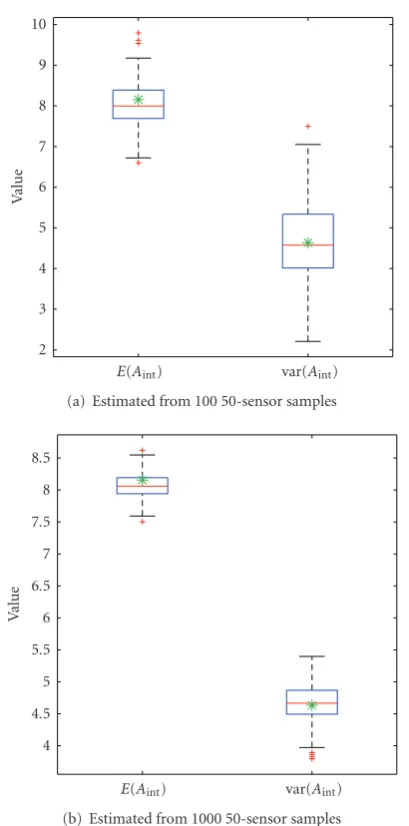
Figures 6(a)and6(b) show box plots of 300 values of
Aint andVint, where each pair of values is estimated from m=100 andm=1000 samples of 50 sensors, respectively. The top and bottom lines of each box represent the upper and lower quartile values of the sample, and the line in-between these two lines represents the sample median; the dashed lines (“whiskers”) extending from the top and bottom of each box represent the spread of the remaining sample, and any plus signs beyond the whiskers represent outliers. The true valuesE(Aint | 1)=8.1540 and var(Aint | 1)= 4.6338 for this example, computed using (40), are indicated in these plots by asterisks. Clearly, the uncertainty in our estimates ofE(Aint|1) and var(Aint|1) decreases with an increase in the number of 50-sensor samples, from 100 to 1000, over the 300 experiments.
4.2. Sensor barrier
Now, consider a nonuniform sensor distribution in the search regionS in which the sensors are distributed in the
x and y dimensions according to the uniform and nor-mal distribution functions, respectively. Specifically, con-sider the sensor x locations distributed independently uniform(−10, 10), and the sensorylocations distributed in-dependently normal(μ,σ) with meanμ=0 and standard de-viationσ=2. Contours of the joint density function fXYare plotted inFigure 7, along with a sample of 50 sensors. This distribution forms a natural barrier against targets moving across the liney=μ; hence, we refer to it as a barrier distri-bution.
The expected value and variance of the area of uncer-taintyAint, given at least one detection, are found using the results of Sections2.1,2.2, and3. These results require the conditional distribution functions FX|ΩT(x) and FY|ΩT(y).
For sensors distributed independently uniform(−10, 10) in the x dimension, we have fX|ΩT(x) = 1/Lx, which gives
FX|ΩT(x)=(x−xΩ)/Lxforxrestricted toΩT. Letφdenote
the standard normal density function (with zero mean and standard deviation one), and let Φ denote its distribution function, so that, for−∞< t <∞,
ϕ(t)=√1 2πexp
−t2/2,
Φ(t)=
t
−∞φ(τ)dτ= 1 2
1 + erft/√2.
var(Aint)
E(Aint)
2 3 4 5 6 7 8 9 10
Va
lu
e
(a) Estimated from 100 50-sensor samples
var(Aint)
E(Aint)
4 4.5 5 5.5 6 6.5 7 7.5 8 8.5
Va
lu
e
(b) Estimated from 1000 50-sensor samples
Figure6: Box plots of 300 experimental values ofE(Aint |1) and
var(Aint|1), each pair estimated from (a) 100 and (b) 1000 samples
of 50 sensors. The asterisks indicate the analytical valuesE(Aint |
1)=8.1540 and var(Aint|1)=4.6338 given by (40), respectively.
It follows that, for sensors distributed independently normal(μ,σ) in the ydimension, we have, for yrestricted toΩT,
fY|ΩT(y)=
1
cσφ
y−μ
σ
, (45)
with normalization constantcgiven by
c=Φ
y
Ω+Ly−μ
σ
−Φ
y
Ω−μ σ
. (46)
Consequently, the conditional distribution function FY|ΩT
for this example is given by
FY|ΩT(y)=
1
c
Φ
y−μ
σ
−Φ
y
Ω−μ σ
. (47)
10 5
0 −5
−10
x
−10 −8 −6 −4 −2 0 2 4 6 8 10
y
Figure7: Sensor location density function for the barrier example, withN =50 sampled sensors.
Since the sensor locations are distributed independently in thexandydimensions, and, moreover, uniformly in the
x dimension, the expected values and variances of Aint(k) and Aint are independent of sensor x location. Figure 8 shows plots of E(Aint | 1) (solid line) and var(Aint | 1) (dashed line) for the midpoint of the target track at y = −6.5,−5.5,. . ., 5.5, 6.5. The endpoints−6.5 and 6.5 are cho-sen so that the bottom and top of the detection regionΩT about the target track coincide with the bottom and top, re-spectively, of the search space S. The theoretical curves in Figure 8are verified experimentally by estimatingE(Aint|1) and var(Aint|1) using the same approach as in the previous example. In this example, instead of estimating the sample statisticsAintandVintform=1000 50-sensor draws and for the detection regionΩTcentered at the origin ofS, we com-pute these statistics form= 1000 50-sensor draws and for the sensor detection regionΩTcentered atx=0 and each of the locationsy= −6.5,−5.5,. . ., 5.5, 6.5. For each of these 14 locations of the detection regionΩTon they-axis, 19 values ofAintandVintare plotted inFigure 8as circles and crosses, respectively. These estimates show good agreement with the theoretical curves.
The analytical and experimental results inFigure 8show some interesting trends. That the expected area of intersec-tion, or area of uncertainty, should decrease monotonically as the target enters the sensor barrier, and then increase at the opposite rate as the target leaves the barrier, is intu-itively obvious, given the symmetry of this example. Few, if any, detections are expected in the tails of the barrier; it fol-lows that the expected value of the area of uncertainty given at least one detection is essentially equal to the area of the detection regionΩT in these regions of S(recall that area (ΩT)=AΩ=14, for this example). Likewise, the area of
14 12 10 8 6 4 2 0
Value −8
−6 −4 −2 0 2 4 6 8
y
Mean Variance
Figure8: Expected value and variance of area of intersection given at least one detection, as functions of theylocation of the midpoint of the detection regionΩT, for the barrier example.
sensor coverage, which, for this example, is the liney=0. In-deed, the expected area of uncertainty given at least one de-tection for this example reaches its minimum value of 3.5552 aty=0.
On the other hand, the behavior of the variance of the area of uncertainty for this example, as displayed by the dashed line inFigure 8, is not so clearly anticipated. In the tails of the barrier, where few, if any, detections are expected, the variance of the area of uncertainty given at least one de-tection tends to zero as the target moves away from the bar-rier. This result is expected, since given exactly one detection, the variance is precisely zero. That the variance should in-crease as the target enters the barrier is also reasonable, as the uncertainty in the area of intersectionAint(k) necessarily increases (from zero) once more than one sensor contributes to the region of intersectionΩint(k), that is, fork >1. How-ever, as the target approaches the center of the barrier, where the sensor density is greatest, the variance of the area of un-certainty decreases, and reaches its minimum value of 3.4601 aty=0. Evidently, for this example, there is a value of sensor density that, when exceeded, yields a decrease in the variance of the area of uncertainty, and otherwise leads to an increase in this variance.
4.3. Arbitrary sensor field
As a next example, consider sensors distributed randomly ac-cording to an arbitrary distribution function, and in partic-ular, one for which the distributions of thexand ysensor locations are dependent. In this case, given the assumptions presented at the end ofSection 2.1, that is, for a long, narrow
detection regionΩT, and for a sensor location density func-tion fXY that does not vary much in thexdimension (the narrow dimension ofΩT), it is reasonable to assume that the sensorx andylocations are locally independent in ΩT, so that
fXY|ΩT(x,y)≈ fX|ΩT(x)fY|ΩT(y), (48)
with the conditional density functionfX|ΩTgiven by (18) and
fY|ΩTgiven by
fY|ΩT(y)=
fXY
X=xΩ+Lx/2,y
yΩ+Ly
yΩ fXY
X=xΩ+Lx/2,ψ
dψ, (49)
for yΩ ≤ y ≤ yΩ+Ly, and fY|ΩT(y) = 0 otherwise. For
convenience in this example, we use the fact that an arbitrary density function can be approximated to an arbitrary level of accuracy by a mixture density function (a weighted sum of density functions) with a sufficient number of terms. In par-ticular, consider theKcomponent, heterogeneous, bivariate normal mixture density function given by
fXY(x,y)=K1
1≤κ≤K
1
ηκφ
x−νκ
ηκ
1
σκφ
y−μ
κ
σκ
, (50)
with component meansνκandμκin thexandydimensions, respectively, with corresponding standard deviationsηκand
σκ, forκ=1,. . .,K. Clearly, thexandycomponents of this density function are dependent. Given this mixture approxi-mation to the density function f, and given the assumptions on the detection regionΩTstated above, the conditional den-sity function fY|ΩT, as given by (49), becomes
fY|ΩT(y)=
1
c
1≤κ≤K
1
ηκ
φ
xΩ+Lx/2−νκ
ηκ
1
σκφ
y−μ
κ
σκ
,
(51)
with normalization constantcgiven by
c=
1≤κ≤K
1
ηκ
φ
xΩ+Lx/2−νκ
ηκ
×
Φ
y
Ω+Ly−μκ
σκ
−Φ
y
Ω−μκ
σκ
.
(52)
The conditional distribution functionFY|ΩT(y) foryΩ≤y≤
yΩ+Lyis obtained by integrating (51) fromyΩtoyyielding
FY|ΩT(y)=
1
c
1≤κ≤K
1
ηκφ
xΩ+Lx/2−νκ
ηκ
×
Φ
y−μ
κ
σκ
−Φ
y
Ω−μκ
σκ
.
(53)
Substituting (53), and the conditional distribution function
FX|ΩT(x)=(x−xΩ)/Lx
Figure 9shows contours of an arbitrary sensor location density function, generated using the mixture density func-tion (50) with K = 5 components, each with equalx and
y standard deviations ηκ = σκ = 2 for allκ, and with x and ymean locations chosen randomly and independently from the uniform(−10, 10) distribution. Also shown in this figure is a sample of 50 sensors. To examine the behavior of the area of uncertainty for the constant velocity target of the previous examples for this particular sensor location den-sity function, we evaluate the expected area of uncertainty,
E(Aint | 1), and the variance of this area, var(Aint | 1), given at least one detection, for the midpoint of the target track atx= −9,−8,. . ., 8, 9 andy= −6.5,−5.5,. . ., 5.5, 6.5. The points in this rectangular grid are chosen so that the union of the detection regionsΩT centered at each point of the grid equals the search spaceS. Figures10(a)and11(a) show the expected value and variance, respectively, of the area of uncertainty given at least one detection from 50 sen-sors distributed according to the density function shown in Figure 9. These quantities are calculated at each point of the grid using the conditional sensor location distribution func-tions given above, and the expressions forE(Aint | 1) and var(Aint | 1) derived in Sections2and3. These theoretical results are verified experimentally by estimatingE(Aint | 1) and var(Aint |1) using the same approach used in the pre-vious two examples. In particular, we estimate the sample statisticsAint andVint form = 1000 50-sensor draws and for the detection regionΩT centered at each grid point. For each of the 19·14=266 locations of the detection regionΩT in the search regionS, the values ofAintandVintare plotted in Figures10(b)and11(b), respectively. For reference, each of the plots in Figures10 and11show the same sample of 50 sensors shown inFigure 9. Also, each of these plots shows the target detection regionΩTcentered at the grid point with the smallest area of uncertainty, that is, the smallest value of
E(Aint); the dashed lines indicate the boundary ofΩT, and the arrow represents the target track over the search interval
T.
As for the previous two examples, the estimatesAintand Vintshow good agreement with the corresponding theoreti-cal values ofE(Aint | 1) and var(Aint | 1). Also, the general trends in the expected value and variance of the area of un-certainty for this arbitrary sensor location distribution are similar to those observed for the sensor barrier. In particular, the expected area of uncertainty tends to decrease monoton-ically as the target approaches regions of dense sensor cov-erage, and increase monotonically as the target leaves these regions. Also, while there is an initial increase in the variance of the area of uncertainty as the target approaches regions of dense sensor coverage, the variance then decreases when a certain level of sensor density is exceeded. Both trends have been consistently observed for other arbitrary sensor loca-tion distribuloca-tions generated from the general mixture den-sity (50), but those results are not included here.
We finally consider a case of a sensor field with >1 re-quired detections. Using an increased value ofin a field de-sign may be performed to reduce the impact of false alarms in large fields, as pointed out in [9]. We consider a sensor field of 50 sensors randomly distributed according to the
10 5
0 −5
−10
x
−10 −8 −6 −4 −2 0 2 4 6 8 10
y
Figure9: Arbitrary sensor location density function, withN =50 sampled sensors.
same process as the previous example. The resulting field is shown inFigure 12. As in the previous example, we examine the behavior of the area of uncertainty for the constant ve-locity target for this particular sensor location density func-tion. However, in this case, we evaluate the expected value of the area of uncertainty given at least four detections, that is,
E(Aint|4). The points in this rectangular grid are chosen in the same manner as forFigure 10.Figure 13showsE(Aint|4) from 50 sensors distributed according to the density func-tion shown inFigure 12. Note that the expected area is very small throughout much of the region, with an average that is noticeably smaller than the previous example (which had the same number of sensors, but only required a single de-tection). This is due to the ability of the track-before-detect kinematic requirements to ignore many detections that are not aligned with three other detections (for this=4 case). The drawback is that it is not very likely to obtain multi-ple detections that provide such track information.Figure 14 shows the corresponding probability of obtaining four detec-tions consistent with the track-before-detect criteria for this example. It is clear from the figure that the regions of highest sensor density contain both the highest probability of obtain-ing multiple detections and the best correspondobtain-ing expected area of uncertainty. Unfortunately, as pointed out in previ-ous work [9], these regions of high sensor density also corre-spond to the greatest probability of false search results. There are also many regions in Figure 13that indicate very good localization accuracy but are very unlikely to receive the nec-essary detections (such as the region near (x,y)=(−4, 1)).
2 2 4 4 4 4 6 6 6 6 6 8 8 8 8 8 8 10 10 10 10 10 10 12 12 12 12 12 10 5 0 −5 −10 x −10 −8 −6 −4 −2 0 2 4 6 8 10 y 2 4 6 8 10 12
(a) Analytical result
2 2 4 4 4 4 4 6 6 6 6 6 8 8 8 8 8 8 10 10 10 10 10 10 12 12 12 12 12 14 14 14 14 14 10 5 0 −5 −10 x −10 −8 −6 −4 −2 0 2 4 6 8 10 y 2 4 6 8 10 12
(b) Experimental result
Figure10: Expected area of intersection given at least one detec-tion.
accuracy often comes at the same locations as increased search effectiveness, but sometimes comes at locations of poor search effectiveness. Neither having good localization accuracy without detections nor having many detections without a sufficiently small area of uncertainty is useful. Even when we have both good search effectiveness and good lo-calization, it is often due to a high density of sensors, which causes more false search reports. Thus we expect these results to be used in careful tradeoffanalyses (as in [13]) to deter-mine the best tradeoffunder design constraints within each specific deployment scenario.
5. CONCLUSIONS
In this paper, expressions were derived for the expected value and variance of the area of uncertainty achieved by employ-ing a track-before-detect search strategy for localizemploy-ing a tar-get moving across a distributed sensor network. The
analyt-0.5 0.5 0. 5 0.5 0. 5 1 1 1 1 1 1. 5 1.5 1. 5 1. 5 1.5 1.5 1.5 2 2 2 2 2 2 2 2.5 2.5 2.5 2.5 2. 5 2.5 2.5 3 3 3 3 3 3 3 3 3 3.5 3.5 3.5 3. 5 3.5 3.5 3.5 3. 5 3.5 3.5 4 4 4 4 4 4 4 4 4 4 4 4.5 4.5 4.5 4.5 4.5 4.5 4.5 4.5 4.5 4.5 4.5 5 5 5 5 5 5 10 5 0 −5 −10 x −10 −8 −6 −4 −2 0 2 4 6 8 10 y
0.5 1 1.5 2 2.5 3 3.5 4 4.5 5
(a) Analytical result
0.5 0.5 0.5 0.5 0.5 1 1 1 1 1 1.5 1.5 1.5 1.5 1.5 1.5 1.5 2 2 2 2 2 2 2 2.5 2.5 2.5 2.5 2.5 2.5 2. 5 2.5 3 3 3 3 3 3 3 3 3 3 3.5 3.5 3.5 3.5 3.5 3.5 3.5 3.5 3. 5 3.5 4 4 4 4 4 4 4 4 4 4 4 4. 5 4.5 4. 5 4.5 4.5 4.5 4.5 4.5 4.5 4.5 4.5 5 5 5 5 5 5 5 10 5 0 −5 −10 x −10 −8 −6 −4 −2 0 2 4 6 8 10 y
0.5 1 1.5 2 2.5 3 3.5 4 4.5 5
(b) Experimental result
Figure11: Variance of area of intersection given at least one detec-tion.
ical expressions were verified by comparison with computa-tional experiments. Examples of uniform, barrier, and arbi-trary field designs were analyzed using these expressions. By studying the analytical expressions for localization accuracy, system designers can developa priorimeasures of eff ective-ness of the resulting sensor system in a parametric manner, thus enabling the optimal setting of critical design parame-ters, such as the placement of sensors within a search area. The analytical nature of these expressions further provides a mechanism for rapid assessment of the area of uncertainty for systems operating in real-time, which is beneficial in as-sessing the potential impact of field degradation on system performance. The use of these expressions within tradeoff analyses for distributed sensor system design is a subject of on-going research.
10 5
0 −5
−10
x
−10 −8 −6 −4 −2 0 2 4 6 8 10
y
Figure 12: A second arbitrary sensor location density function, withN =50 sampled sensors.
1.5 1.5
1.5 1.5
2 2
2
2
2
2 2
2.5
2.5
2.5 2.5
2.5 2.5
2.5
2.5
2.5
3 3
3
3 3
3
3
3.5
3.5
3.5
3.5
4
4
4 4.5
10 5
0 −5
−10
x
−10 −8 −6 −4 −2 0 2 4 6 8 10
y
1.5 2 2.5 3 3.5 4 4.5
Figure13: Expected area of intersection given at least four detec-tions for the sensor density inFigure 12.
sensor detections in a probabilistic manner, this method is useful as a tool for designing sensor fields to track moving targets. The cases in this paper have been limited to single targets; the extension to multiple targets is a known benefit of track-before-detect strategies and is a subject of future in-terest. Other future areas of application of these results are in field design guidance that trades-offfalse alarm performance and expected localization accuracy, as well as the extension to heterogeneous sensor fields.
APPENDIX
Before proceeding to the proof ofLemma 2, we recall some facts about the beta distribution. The interested reader is
re-0.1
0.1 0.1
0.1
0.1
0.1
0.1
0.1
0.2 0.2
0.2
0.2 0.2
0.2
0.2 0.3
0.3
0.3
0.3 0.3
0.3
0.3
0.4
0.4 0.4
0.4
0.4 0.5 0.5
0.5 0.5
0.5
0.6 0.6
0.6
0.7 0.7
10 5
0 −5
−10
x
−10 −8 −6 −4 −2 0 2 4 6 8 10
y
0.1 0.2 0.3 0.4 0.5 0.6 0.7 0.8 0.9
Figure14: Probability of obtaining four sensor detections during a track interval for the sensor density inFigure 12.
ferred to Casella and Berger [14] for more details. The beta distribution with parameters λ > 0 and μ > 0, denoted beta(λ,μ), is a continuous distribution with density function
β(x;λ,μ) for 0≤x≤1 given by
β(x;λ,μ)= xλ−1(1−x) μ−1
B(λ,μ) , (A.1)
where the constantB(λ,μ) can be written in terms of gamma functions, specificallyB(λ,μ)=Γ(λ)Γ(μ)/Γ(λ+μ). Further-more, ifXis a random variable distributed beta(λ,μ), then the expected value and variance ofXare given by
E(X)= λ
λ+μ, var(X)=
λμ
(λ+μ)2(λ+μ+ 1), (A.2)
respectively. The expressions in (A.1) and (A.2) are required within the following proof. We now complete the proof of Lemma 2.
Proof ofLemma 2.Since sensor x location is distributed
uniform(xΩ,xΩ+Lx) inΩT, we have that
FX|ΩT(x)= ⎧ ⎪ ⎪ ⎪ ⎪ ⎨ ⎪ ⎪ ⎪ ⎪ ⎩
0, x < xΩ, x−xΩ
Lx , xΩ≤x≤xΩ+Lx, 1, x > xΩ+Lx.
(A.3)
Expressions (24) can be obtained by substituting this defini-tion for the condidefini-tional distribudefini-tion of sensorxlocation into (15) and (22), respectively, and computing the necessary in-tegrals. However, it is easier to first prove that the stronger statementdx(k)/Lxis distributed beta(k−1, 2), and then use the expressions in (A.2) for the mean and variance of a beta distributed random variable to show (24).