Volume 2009, Article ID 534137,13pages doi:10.1155/2009/534137
Research Article
Non-Cancellation Multistage Kurtosis Maximization with
Prewhitening for Blind Source Separation
Xiang Chen,
1Chong-Yung Chi,
2Tsung-Hui Chang,
2and Chon-Wa Wong
21Wireless Center, Research Institute of Information Technology, Tsinghua University, Beijing 100084, China 2Department of Electrical Engineering, Institute of Communications Engineering, National Tsing Hua University,
Hsinchu 30013, Taiwan
Correspondence should be addressed to Xiang Chen,[email protected]
Received 23 September 2008; Revised 4 December 2008; Accepted 13 January 2009
Recommended by S. Makino
Chi et al. recently proposed two effective non-cancellation multistage (NCMS) blind source separation algorithms, one using the turbo source extraction algorithm (TSEA), called the NCMS-TSEA, and the other using the fast kurtosis maximization algorithm (FKMA), called the NCMS-FKMA. Their computational complexity and performance heavily depend on the dimension of multisensor data, that is, number of sensors. This paper proposes the inclusion of the prewhitening processing in the NCMS-TSEA and NCMS-FKMA prior to source extraction. We come up with four improved algorithms, referred to as the PNCMS-TSEA, the PNCMS-FKMA, the PNCMS-TSEA(p), and the PNCMS-FKMA(p). Compared with the existing NCMS-TSEA and NCMS-FKMA, the former two algorithms perform with significant computational complexity reduction and some performance improvements. The latter two algorithms are generalized counterparts of the former two algorithms with the single source extraction module replaced by a bank of source extraction modules in parallel at each stage. In spite of the same performance of PNCMS-TSEA and PNCMS-TSEA(p) (PNCMS-FKMA and PNCMS-FKMA(p)), the merit of this parallel source extraction structure lies in much shorter processing latency making the PNCMS-TSEA(p) and PNCMS-FKMA(p) well suitable for software and hardware implementations. Some simulation results are presented to verify the efficacy and computational efficiency of the proposed algorithms.
Copyright © 2009 Xiang Chen et al. This is an open access article distributed under the Creative Commons Attribution License, which permits unrestricted use, distribution, and reproduction in any medium, provided the original work is properly cited.
1. Introduction
Blind source separation (BSS) (or independent component analysis), a problem to extract unknown sources only from observations over multiple sensors, has received wide atten-tion in many areas such as array signal processing, wireless communications, and biomedical signal processing. There have been a number of statistical BSS algorithms reported in the open literature basically including algorithms using second-order statistics (SOS) (known as correlations) [1– 3], algorithms using higher order statistics (HOS) (known as cumulants) [4–18], and a variety of linear and nonlinear algorithms using principles such as maximum-likelihood method and maximum entropy [4, 5, 19], or using char-acteristics and features of source signals and the mixing matrix such as nonstationarity and nonnegativity or their combinations [20–23]. SOS-based algorithms such as the
algorithm for multiple unkown signals extraction (AMUSE) proposed by Tong et al. [2, 6], the second-order blind identification (SOBI) algorithm proposed by Belouchrani et al. [1], and the matrix-pencil approach proposed by Chang et al. [3] generally require the sources to be temporally colored and spatially uncorrelated with different power spectra, while HOS-based algorithms generally require the sources to be non-Gaussian though their power spectra are allowed to be the same. The AMUSE and SOBI algorithms further requireP > K(Pis the number of sensors,Kis the number of sources) and the noise correlation matrix given or estimated in advance, while the matrix-pencil approach requiresP ≥K instead ofP > K without need of the noise correlation matrix [3].
example, Hyv¨arinen and Oja’s fast fixed-point algorithm (also called the FastICA) [11], Ding and Nguyen’s kurtosis maximization algorithm (KMA) [15], Shalvi and Weinstein’s superexponential algorithm (SEA) [13, 14] and Chi and Chen’s fast kurtosis maximization algorithm (FKMA) [16]. The FKMA also makes use of the SEA [17] and therefore shares the superexponential convergence rate, and mean-while guarantees the convergence for finite data length and finite signal-to-noise ratio (SNR). However, the smaller the normalized kurtosis magnitude of the extracted source signal, the worse the performance of these algorithms. Chi and Peng recently proposed another BSS algorithm, called the turbo source extraction algorithm (TSEA) [24], whose performance is quite insensitive to the kurtosis magnitude of the extracted source signal. To extract all the unknown sources, a number of the BSS algorithms have been used in conjunction with a multistage successive cancellation (MSC) procedure for the extraction of all the unknown sources in a one-by-one manner. This procedure, however, is susceptible to error propagation accumulated at each stage and thus limits the quality of extracted source signals at later stages. To circumvent this error propagation problem, Chi and Peng [24] further proposed a non-cancellation multistage (NCMS) framework for FKMA and TSEA, named the NCMS-FKMA and NCMS-TSEA, respectively. It has been shown [24] that the NCMS-FKMA and NCMS-TSEA significantly outperform their MSC-based counterparts as well as some existing BSS algorithms which do not involve any successive deflation procedure. However, the compu-tational complexity and performance of both the NCMS-TSEA and the NCMS-FKMA are heavily dependent on the dimension of multisensor data (i.e., the number of sensors).
In the paper, the prewhitening processing which is effective for dimension reduction and noise reduction is performed prior to source separation using the NCMS-TSEA and NCMS-FKMA, straightforwardly providing two computationally improved algorithms, referred to as the PNCMS-TSEA and the PNCMS-FKMA. The proposed PNCMS-TSEA and PNCMS-FKMA benefit not only from the prewhitening processing but also from their internal computational complexity reduction resultant from the fact that the mixing matrix is converted to a unitary mixing matrix. Specifically, the column vector estimation of the unknown mixing matrix and the computation of orthogonal complimentary projection matrix required in NCMS-TSEA and NCMS-FKMA can be substantially simplified in their PNCMS counterparts.
Since the NCMS-based algorithms requireK stages to extract all of theK source signals, they would yield a long processing latency when K is large. Aiming at reducing the processing latency, we further develop two algorithms, namely PNCMS-TSEA(p) and PNCMS-FKMA(p), that are able to extract all the sources with the number of stages that is much smaller thanK (typically less than 3 forK ≤ 10). The idea is to employ multiple source extraction modules at each stage for parallel source extraction, and meanwhile maintain the same source extraction performance. Thanks to the unitary mixing matrix involved in the prewhitened data, we find that column vectors of an arbitrary unitary matrix
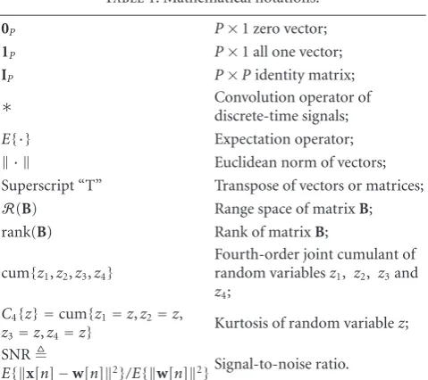
Table1: Mathematical notations.
0P P×1 zero vector;
1P P×1 all one vector;
IP P×Pidentity matrix;
∗ Convolution operator ofdiscrete-time signals;
E{·} Expectation operator;
· Euclidean norm of vectors;
Superscript “T” Transpose of vectors or matrices;
R(B) Range space of matrixB;
rank(B) Rank of matrixB;
cum{z1,z2,z3,z4}
Fourth-order joint cumulant of random variablesz1, z2, z3and
z4;
C4{z} =cum{z1=z,z2=z,
z3=z,z4=z} Kurtosis of random variablez;
SNR
E{x[n]−w[n]2}/E{w[n]2}Signal-to-noise ratio.
can practically serve as a set of initial conditions (spatial filters) for initializing iterative FKMAs or TSEAs operating in parallel. As a result, the use of the parallel TSEA (FMKA) source extraction modules in PNCMS-TSEA(p) (PNCMS-FKMA(p)) can effectively extract most of the unknown sources at each and every stage. In fact, the PNCMS-TSEA(p) and PNCMS-FKMA(p) are, respectively, the generalized counterparts of the PNCMS-TSEA and PNCMS-FKMA since the former two algorithms reduce to the latter two algorithms if they are artificially constrained to only one source signal extraction at each stage. The performance and computational complexity improvements of the proposed PNCMS-TSEA and PNCMS-FKMA as well as the reduced processing latency of the TSEA(p) and PNCMS-FKMA(p) are verified by computer simulations.
The organization of the rest of this paper is as fol-lows. In Section 2, we present the BSS problem and some general model assumptions used. In Section 3, the exist-ing FKMA, TSEA, NCMS-TSEA, and NCMS-FKMA are briefly reviewed. After the presentation of the proposed PNCMS-TSEA and PNCMS-FKMA in Section 4.1, their parallel source extraction counterparts, PNCMS-TSEA(p) and PNCMS-FKMA(p), are presented in Section 4.2. In
Section 5, some simulation results are then presented to
demonstrate the effectiveness and computational complexity advantages of the proposed algorithms. Finally, some conclu-sions are drawn inSection 6.
2. Problem Statement and Assumptions
For ease of later use, let us define the notations shown in
Table 1.
Given a set of P sensor measurements, denoted by a
the following instantaneous (or memoryless) multiple-input multiple-output (MIMO) model:
x[n]=As[n] +w[n]
= K
k=1
aksk[n] +w[n],
(1)
where A = [a1,a2,. . .,aK] is an unknown P×K mixing matrix, and w[n] = [w1[n],w2[n],. . .,wP[n]]T is a P×1 noise vector. Here,x[n],A,s[n], andw[n] are assumed to be real valued for simplicity. As made in [24], some general assumptions for the MIMO system model in (1) are given as follows.
(A1) The unknownP×Kmixing matrixAis of full column rank (i.e.,P≥Kand rank(A)=K), andKis known a priori.
(A2) Each source signalsk[n],k ∈ {1, 2,. . .,K}, is a non-Gaussian causal linear process, that is,sk[n] can be modeled as the output of a causal stable linear time-invariant systembk[n] as follows:
sk[n]=bk[n]∗uk[n]
= ∞
m=0
bk[m]uk[n−m],
(2)
where uk[n] is a stationary, zero-mean, non-Gaussian, independent, and identically distributed (i.i.d.) process with a nonzero kurtosis given by [25]
C4
uk[n]
=cumuk[n],uk[n],uk[n],uk[n]
=Euk[n]4
−3Euk[n]2
2 . (3)
The uk[n], k = 1,. . .,K, are mutually statistically independent.
(A3) The noisew[n] is zero-mean Gaussian and is statisti-cally independent ofs[n].
Letvbe aP×1source extraction filter(a spatial filter) for processing the signalx[n]. Then the filter output is given by
e[n]=vTx[n]. (4)
Source separation algorithms are essentially developed for designing a set ofK source extraction filters, each of which extracts a distinct source signal. Next, let us briefly review the FKMA proposed by Chi and Chen [16,17], the TSEA, the NCMS-FKMA, and the NCMS-TSEA proposed by Chi and Peng [24], respectively.
3. Review of FKMA, TSEA, NCMS-FKMA,
and NCMS-TSEA
3.1. FKMA [16]. The FKMA is an iterative algorithm for finding the optimum spatial filter v by maximizing the magnitude of normalized kutosis ofe[n] [12,15]:
J(v)=J(e[n])=C4{e[n]} Ee[n]22.
(5)
With the assumptions (A1) and (A2) and the noise-free assumption, the optimum spatial filter v is able to extract one of theKsource signals, that is,e[n]=αksk[n] for some k∈ {1, 2,. . .,K}, whereαkis an unknown nonzero constant. At theith iteration, this algorithm updates
v(i)= R
−1
x d
e(i−1)[n]
R−1
x d
e(i−1)[n] (6)
(basically with superexponential convergence rate), where Rx = E{x[n]xT[n]} is the correlation matrix of x[n],
e(i−1)[n]=(v(i−1))Tx[n] and
de(i−1)[n]=cume(i−1)[n],e(i−1)[n],e(i−1)[n],x[n] =Ee(i−1)[n]3x[n]−3Ee(i−1)[n]2
×Ee(i−1)[n]x[n].
(7)
In case of J(v(i)) < J(v(i−1)), a gradient-type algorithm is
used to update v(i) instead. This iterative algorithm stops
when a preassigned convergence tolerance is reached. The computational load of the FKMA is determined by the total number of iterations spent and the dimension ofx[n].
3.2. TSEA [24]. The TSEA is a cyclically iterative spatial-temporal processing algorithm which maximizes
J(vTSEA[n])=J(ε[n]), where
vTSEA[n]=vg[n],
ε[n]=vTTSEA[n]∗x[n]=vT
L
m=0
g[m]x[n−m]
, (8)
in whichg[n] is a single-input single-output temporal filter of order equal toL, that is,g[n]=/0, n=0,. . .,L. At theith cycle, the TSEA consists of the following two steps.
(S1) Compute y(i−1)[n] = g(i−1)[n]∗x[n] followed by
processingy(i−1)[n] using the FKMA(s)(withv(i−1)as
the initial condition) to obtain the optimum spatial filterv(i)andε[n]=(v(i))T
y(i−1)[n]. The superscript
“(s)” in FKMA(s)indicates that the FKMA is used for the design of the spatial filterv.
(S2) Compute e[n] = (v(i))T
x[n] and then find the optimum temporal filter gi = [g(i)[0],g(i)[1],. . ., g(i)[L]]T
using the FKMA(t) (withgi−1as the initial
condition) and obtainε[n]=e[n]∗g(i)[n]=gT
ie[n], where e[n] = [e[n],e[n−1],. . .,e[n−L]]T. The superscript “(t)” in FKMA(t)indicates that the FKMA
is used for the design of the temporal filterg[n].
FKMA. Therefore, the TSEA outperforms the FKMA. For extraction of all the unknown sources without involving any successive cancellation processing, the NCMS-TSEA and NCMS-FKMA have been proposed in [24] and are briefly reviewed in the next subsection.
3.3. NCMS-TSEA and NCMS-FKMA [24]. The
NCMS-TSEA is a non-cancellation multistage source separation algorithm which, at stage, extracts a distinct source signal estimate, denoted by e[n], and obtains the associated column vector estimate of A, denoted by a. Let C = [a1,a2,. . .,a−1] and let C⊥ be aP ×P projection matrix for whichR(C⊥) is orthogonal toR(C). The NCMS-TSEA includes the following steps.
(T1) Set=0,C⊥1 =IPandx1[n]=x[n].
(T2) Updateby+1. If≥2, obtainC⊥ through singular value decomposition (SVD) ofC, and compute the projected data x[n] = C⊥x[n] (which basically consists of all the contributions associated with the sources that have not yet been extracted).
(T3a) Source extraction with x[n] (constrained source extraction). Obtain vTSEA[n] = υg[n], ε[n] = vTTSEA[n]∗x[n], and e[n] = υTx[n] using the TSEA. Then estimate the associated column vector in the mixing matrix by the input-output-cross-correlation (IOCC) method [16], that is,
a= E
x[n]e[n]
Ee[n]2
(9)
and obtain
v=C⊥υ. (10)
(T3b) Source extraction with x[n] (unconstrained source extraction). Obtain the optimumvTSEA[n]=vg[n], ε[n]= vTTSEA[n]∗x[n], ande[n] =vTx[n] using the TSEA (withvandg[n] obtained in (T3a) as the initial conditions forvandg[n], resp.).
(T4) If < K, go to (T2); otherwise, all the source signal estimates{e[n],=1, 2,. . .,K}have been obtained.
The NCMS-FKMA is nothing but a special case of the NCMS-TSEA, where the TSEA is replaced by the FKMA in (T3a) and (T3b). The latter outperforms the former simply because the TSEA performs better than the FKMA. It should be mentioned that the TSEA and NCMS-FKMA exhibit better performance than their counterparts involving MSC procedure because they are free from error propagation [24].
4. Improvements of NCMS-TSEA and
NCMS-FKMA by Prewhitening
In the section, we present the TSEA and PNCMS-FKMA by incorporating the prewhitening processing in the NCMS-TSEA and NCMS-FKMA, respectively. The
prewhitening processing transforms the P × K mixing matrix A into a K × K unitary mixing matrix. As we will show in the first subsection that this simple prepro-cessing not only can reduce the computational load in source extraction that follows but also can improve the source extraction performance. In the later subsections, we further present a parallel implementation counterpart for the PNCMS-TSEA (PNCMS-FKMA), referred to as the PNCMS-TSEA(p) (PNCMS-FKMA(p)), that is able to extract multiple unknown sources in parallel at each stage and thus able to significantly shorten the processing latency.
4.1. NCMS-TSEA with Prewhitening (PNCMS-TSEA). In the subsection, let us present the TSEA and PNCMS-FKMA that share the advantages of dimension reduction and noise reduction together with further internal computational complexity reduction over the TSEA and NCMS-FKMA. The idea is motivated by the following lemma.
Lemma 1. Suppose that the mixing matrixAin x[n]given by(1)is a unitary matrix (i.e.,P = KandAAT = I
K) and that the assumptions (A1), (A2) and the noise-free assumption hold. Then the optimum source extraction filtervby finding a local maximum ofJ(v)(see(5)) is given byv= ±akfor some k∈ {1, 2,. . .,K}, and the associated extracted source signal is
e[n]=vTx[n]= ±s k[n].
The proof ofLemma 1is presented in the Appendix. This lemma implies that when the mixing matrixAis a unitary matrix, the optimum source extraction filtervitself provides an estimate of the column vector ak associated with the extracted sourcesk[n], and thereby the estimation ofak in (T3a) of the NCMS-TSEA is not needed any more. Moreover, step (T2) in the NCMS-TSEA can be fulfilled without SVD.
ByLemma 1, one can simply setC=[v1,v2,. . .,v−1] which
is a semiunitary matrix (i.e., (C)TC =I−1), and thus the
correspondingC⊥ is given by [26]
C⊥ =IK−CCT. (11)
Fortunately, the widely used prewhitening processing through eigenvalue decomposition of the correlation matrix Rx =E{x[n]xT[n]}for both dimension reduction and noise reduction ofx[n] can transform theP×K mixing matrix A into a K ×K unitary matrix [9, 11]. With the above computational reduction, noise reduction, and the removal of column vector estimation and SVD in NCMS-TSEA, the proposed PNCMS-TSEA is summarized as follows.
(P1)Prewhitening. Obtain the prewhitening matrix W = [h1/
(λ1−σw2),. . .,hK/
(λK−σw2)]T, where λ1,. . .,λK are the K largest eigenvalues of Rx and h1,. . .,hK are the associated eigenvectors. The noise variance estimateσ2
wis obtained as the average of the otherP−K eigenvalues ofRx. Updatex[n] by the prewhitened dataWx[n] (K×1 vector).
(P3) Updateby+ 1. If≥2, calculateC⊥ using (11), where C = [v1,v2,. . .,v−1] and then obtain the
projected datax[n]=C⊥x[n].
(P4) Perform source extraction with the projected data x[n] as in (T3a) followed by source extraction with x[n] as in (T3b) of the NCMS-TSEA to obtain v (normalized byv =1) ande[n].
(P5) If < K, go to (P3); otherwise, all the source signal estimates{e[n],=1, 2,. . .,K}have been obtained.
Three remarks about the proposed PNCMS-TSEA are as follows.
(R1) The proposed PNCMS-TSEA basically extracts all the sources through the same signal processing procedure as the NCMS-TSEA except that (P3) for the former is much simpler than (T2) for the latter at each stage, and meanwhile the SVD is not needed in (P3) and no column vector estimation of the mixing matrix is involved in (P4). The inclusion of the prewhitening processing (P1) for the former substantially reduces the computational complexity because the major processing involving FKMA in (P4) is dependent upon the dimension K of the prewhitened data instead of the dimensionP (≥K) of the original data, especially when P K. The extra computational load due to the prewhitening processing in (P1) is negligible compared with the amount of computation load reduction in source extraction.
(R2) The performance of the proposed PNCMS-TSEA is basically similar to that of the NCMS-TSEA because the former can be thought of as a more efficient implementation based on the same source sepa-ration criterion (kurtosis maximization). However, some performance improvements of the proposed PNCMS-TSEA over the NCMS-TSEA can still be gained for low SNR because twofold noise reduction is performed: Prewhitening processing and source extraction in lower dimension space.
(R3) With the TSEA used in (P4) replaced by the FKMA, the proposed PNCMS-TSEA reduces to the one, called the PNCMS-FKMA. The performance of the former is also superior to the latter simply due to the better performance of the TSEA over the FKMA.
4.2. PNCMS-TSEA and PNCMS-FKMA with Parallel Source Separation Structure. Since the NCMS algorithms extract only one source at each stage, the total number of stages spent by the NCMS algorithms for extracting all the source signals equals the total number of unknown sources. If K
is large, a long processing latency is apparently inevitable. In order to reduce the processing latency, in the subsection, by making use of a parallel source extraction structure for the PNCMS-TSEA and PNCMS-FKMA we propose two more algorithms, referred to as the PNCMS-TSEA(p) and PNCMS-FKMA(p), respectively. The PNCMS-TSEA(p) (PNCMS-FKMA(p)) basically has the same performance as
the PNCMS-TSEA (PNCMS-FKMA), but at each stage the former uses multiple TSEA (FKMA) modules in parallel for multiple source extractions followed by source signal classification. The parallel source extraction will be shown to be effective in cutting down the total number of stages in extracting all the source signals and thus effective in shortening the processing latency.
4.2.1. Initial Conditions for Parallel Source Extraction. Prior to presenting the proposed PNCMS-TSEA(p) in detail, let us first address the idea of how to efficiently extract as many distinct source signals as possible via the use of parallel TSEA modules at each stage. Since different initial conditions for the spatial filter v to initialize either FKMA or TSEA may result in different source signals to be extracted, this fact implies the need of proper initial conditions for each TSEA module. Thanks to the prewhitening processing which transforms the mixing matrix Ainto a unitary matrix, we empirically found that K distinct initial conditions taken from theK columns of an arbitraryK ×K unitary matrix can end up with distinct source signals to be extracted with a high fraction ofK. To illustrate this, given aK×Kunitary mixing matrixA = [a1,. . .,aK] we define aK×K matrix B=[b1,. . .,bK] in which
bj=arg max
a∈Av T
ja=arg min
a∈Avj−a 2
, j=1, 2,. . .,K,
(12)
where
A=±a1,. . .,±aK
, (13)
andV =[v1,. . .,vK] is an arbitraryK×K unitary matrix. Then the column vector bj represents the column vector in Athat is closest tovj. Hence by maximizing J(v) with vj as the initial condition, the optimum spatial filtervmay well converge tobjimplied byLemma 1and the associated outputej[n]= bTjx[n] ∈ {±s1[n],. . .,±sK[n]}. Therefore, one can anticipate that the larger the number of distinct column vectors inB, the larger the number of distinct source signals that will be extracted byKTSEA (or FKMA) modules operating simultaneously. In order to get some idea about the average number of distinct column vectors inB, denoted asd(B), let us present some simulation results for a given
K×Kunitary matrixAfor the cases ofK =2, 3,. . ., 10. For eachK×K mixing matrixA, 105 unitary matricesVwere
randomly generated and the associated matricesB in (12) were calculated.Table 2lists the obtained simulation results ofd(B).
From Table 2, it can be observed that there are larger
than 80% distinct columns in B on average for K ≤ 10, indicating that the use of the K columns of an arbitrary
Table2: Average number of distinct columns inB,d(B), forK=2 toK=10.
K 2 3 4 5 6 7 8 9 10
d(B) 2 2.8499 3.6517 4.447 5.2262 5.9683 6.7247 7.469 8.181
d(B)/K(%) 100 95 91.29 88.94 87.1 85.26 84.06 82.99 81.81
matrix), the total number of stages required to extract all of the source signals can be appreciably reduced, thus effectively reducing the processing latency.
Now let us elaborate upon the parallel NCMS structure of PNCMS-TSEA(p). Suppose that before stage, there have beeni() distinct source signals already extracted, and thus at stagethere are
k()=K−i() (14)
source signals yet to be extracted. Let
C=
C−1 C−1
, (15)
where C−1 contains the spatial filters that are obtained at
stage−1 andC−1 contains all the obtained spatial filters
before stage−1. As illustrated inFigure 1, for the projected data x[n] = C⊥x[n] at stage , the proposed PNCMS-TSEA(p) employsk() parallel TSEA modules each using a distinct column vector of an arbitraryK×Kunitary matrix as the initial condition to obtaink() source signal estimates. Denote by υr, r = 1,. . .,k(), the k() source extraction filters and letvr =C⊥υr (by (10)) forr =1,. . .,k(). Since the k() extracted sources may not be distinct altogether, they are needed to identify those source signal estimates and spatial filters associated with distinct sources. To this end, a source classification algorithm that follows thek() TSEA modules as shown inFigure 1is presented next.
4.2.2. Source Signal Classification. According to Lemma 1, the obtained spatial filtersvr, r = 1,. . .,k() are also the estimates of the column vectors of the unknown unitary mixing matrixA. Consider the spatial filtersviandvj that maximizeJ(e[n]=vTx[n]) with the respective outputs given
by
ei[n] =
viTx[n], (16)
ej[n] =
vj
T
x[n]. (17)
Under the assumptions (A1), (A2) and the noise-free assumption, the correlation ofei[n] andej[n] is given by
Eei[n]ej[n]
=viTEx[n]xT[n]v j
=vi
T K
k=1 γkakaTk
vj
= K
k=1 γk
vi
T
ak
aTkvj
,
(18)
whereγk =E{|sk[n]|2}, k=1,. . .,K, are the source signal powers. Sincevi,vj∈A(see (13)) byLemma 1and allakare orthonormal to each other, (18) implies that
Eei[n]ej[n]
=
0 if vi= ±/ vj ±γi if vi= ±vj.
(19)
Therefore, the distinct extracted source signals can be iden-tified according to the pairwise correlation of v1,. . .,vk().
In other words, if |(vi)Tvj| > η (a threshold between 0 and 1), ei[n], and ej[n] are actually estimates of the same source signal. With our experience, η = 0.5 is a good choice for signal classification. Based on the above analysis, we present a source signal classification algorithm
in Table 3, where j() represents the number of distinct
source signals among the k() extracted sources, and (v1,g1[n]), (v2,g2[n]),. . ., (vj(),gj()[n]) are the associated
spatial filters and temporal filters. Note that the compu-tational load for source signal classification is negligible compared with source extraction. As illustrated inFigure 1, the PNCMS-TSEA(p) at stage ends up with the j() unconstrained source extractions using j() parallel TSEA modules with (v1,g1[n]), (v2,g2[n]),. . ., (vj(),gj()[n]) as
the initial conditions. The PNCMS-TSEA(p) then repeats the above processing procedures (namely,k() parallel TSEA source extractions with the projected signal x[n], source classification andj() parallel TSEA source extractions with the nonprojected signalx[n]) stage by stage until all theK
source signals are extracted.
4.2.3. The Proposed PNCMS-TSEA(p). Here let us summa-rize the detailed steps of the proposed PNCMS-TSEA(p) as follows.
(F1)Prewhitening. Obtain prewhitening matrix W and then updatex[n] by the prewhitened dataWx[n] as in (P1) of the PNCMS-TSEA.
(F2) Seti(0)= j(0)==0,C⊥1 =IKandx1[n]=x[n].
(F3) Updateby+ 1, seti()=i(−1) +j(−1) (total number of sources having been extracted) andk()= K−i() (number of sources yet to be extracted). If≥
2, obtainCandC⊥ using (15) and (11), respectively, and then obtain the projected datax[n]=C⊥x[n].
(F4a) Parallel source extractions with the projected data x[n]: obtaink() pairs of spatial and temporal filters {(υr,gr[n]),r =1,. . .,k()}by using thek() TSEA modules in parallel with the initial condition pairs
Prewhitened signal
x[n]
C−1
C=[C−1C−1] C⊥ =IK−CCT x[n]=C⊥x[n]
PNCMS-TSEA(p): i()=i(−1) +j(−1) k()=K−i() PNCMS-TSEA: i()=−1 k()=1
x[n]
υ(0)1
TSEA
υ1
g1[n]
υ(0)2
TSEA υ
2
g2[n] . . .
υ(0)k()
TSEA υ
k() gk() [n] g(0)[n]=δ[n]
. . .
· · ·
g1[n]
v1
Source signal classification (Table 3)
C⊥
. . .
. . . TSEA
TSEA
ei()+1[n]
ei()+j()[n]
gj()[n]
vj()
C=[v1,· · ·,vj()]
Figure1: The source extraction processing of the proposed PNCMS-TSEA(p) and PNCMS-TSEA at stage.
Given: the obtained pairs of spatial and temporal filter (v
r=C⊥υr,gr[n]), r=1,. . .,k(), and a thresholdη >0. Step 1: Setp=0,S= {(v
r,gr[n]),r=1,. . .,k()}
andS1= {vr,r=1,. . .,k()}.
Step 2: Updatepbyp+ 1. Ifp≥2,Sp=S1\ {C1∪ · · · ∪Cp−1}. Step 3: Choose an arbitrary reference spatial filter
up∈Sp. Then find the set Cp=v|v∈Sp,uTpv> η
.
Step 4: Obtain the pair (vp,gp[n])∈Swhere vp=arg max
v∈Cp
Je[n]=vTx [n]. Step 5: Repeat Step 2 to Step 4 untilip=1Ci=S1,
wherej()=pis the total number of distinct sources.
Table3: Source signal classification algorithm.
(F4b) Obtain the pairs of spatial and temporal filters
{(vr,gr[n]),r = 1,. . .,j()}using the source signal classification algorithm in Table 3 and set C = [v1,. . .,vj()], where j() is the number of distinct
sources extracted at stage.
(F4c) Parallel source extractions with the prewhitened data x[n] obtained in (F1): obtainei()+1[n],ei()+2[n],. . ., ei()+j()[n] by using j() TSEA modules in parallel
with the pairs {(vr,gr[n]),r = 1,. . .,j()} as the initial conditions.
(F5) Ifi() +j()< K, go to (F3); otherwise, all the source signal estimates {eq[n],q = 1, 2,. . .,K} have been obtained.
Five remarks about the proposed PNCMS-TSEA(p) are given as follows.
(R5) The proposed PNCMS-TSEA(p) basically extracts all the sources through the parallel NCMS sig-nal processing and shares the same performance and computational complexity advantages of the PNCMS-TSEA due to the prewhitening processing as described in (R1) and (R2).
(R6) The proposed PNCMS-TSEA(p) reduces the process-ing latency in separation of all theK source signals since it can simultaneously extract as many distinct sources as possible at each stage in contrast to a single source extracted by the NCMS-TSEA/PNCMS-TSEA at each stage. Specifically, for the scenario within ten sources (K≤10), we empirically found that all of the sources can be extracted within 3 stages.
the source classification algorithm used in (F4b), the proposed TSEA(p) reduces to the PNCMS-FKMA(p), and again the former is superior to the latter owing to the superior performance of TSEA. (R8) The proposed PNCMS-TSEA (PNCMS-FKMA) can
also be thought of as a special case of the proposed PNCMS-TSEA(p) (PNCMS-FKMA(p)). In particu-lar, by setting k() = 1 and i() = −1 at (F3), the PNCMS-TSEA(p) reduces to the PNCMS-TSEA presented inSection 4.1, that is, the bank of parallel source separation modules inFigure 1is replaced by a single source separation module.
(R9) The proposed parallel NCMS structure is not limited to the use with the FKMA and the TSEA. Instead, it can be used with any BSS algorithms which basically extract one source at each stage, such as the KMA [13] and the SEA [12], to avoid the error propagation issue in multistage source deflation on one hand, and reduce the processing latency on the other hand. The FastICA [11], though extracting one source at each stage, cannot be directly applied to the proposed parallel NCMS structure because from the second stage (≥2), the projected signal
x[n]=C⊥x[n]=C⊥As[n] (20)
involves a mixing matrixC⊥Awhich is no longer a unitary matrix required by FastICA. Therefore, the FastICA cannot be used unless further prewhitening processing is applied to x[n].
5. Simulation Results
To justify the efficacy of the proposed BSS algorithms, namely the PNCMS-TSEA, PNCMS-FKMA, PNCMS-TSEA(p), and PNCMS-FKMA(p), three parts of simulation results are presented in the section. The first part considers the performance comparison of the proposed BSS algorithms with the existing NCMS-TSEA and NCMS-FKMA for the case of all the source signals with the same power spectrum. The second part focuses on the performance comparison of the proposed BSS algorithms with the existing FastICA [11], SOBI [1], and AMUSE [2] for the case of all the source signals with different power spectra. The third part then presents some results on the computational complexity and processing latency of the proposed four algorithms.
The i.i.d. ui[n]’s used for generating si[n]’s were equiprobable random binary sequences of±1, and the fifth-order FIR modelsbi[n]’s in [3]
bi[n]=exp − n + 1 10·μi
, n=0, 1,. . ., 5 (21)
were used for the generation of si[n] in (2), where the parameter μi specifies the power spectrum of the source signal si[n]. The noise vector w[n] was real, zero-mean, spatially independent, and temporally white Gaussian dis-tributed with covariance matrix equal toσ2
wIP. Three mixing
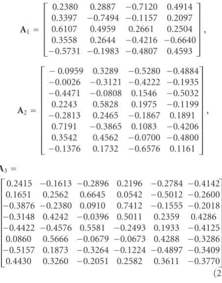
matrices, denoted byA1(a 5×4 matrix taken from [3]),A2
(an 8×4 matrix), andA3(an 8×6 matrix) were considered
in the simulations as follows:
A1=
⎡ ⎢ ⎢ ⎢ ⎢ ⎢ ⎣
0.2380 0.2887 −0.7120 0.4914 0.3397 −0.7494 −0.1157 0.2097 0.6107 0.4959 0.2661 0.2504 0.3558 0.2644 −0.4216 −0.6640
−0.5731 −0.1983 −0.4807 0.4593
⎤ ⎥ ⎥ ⎥ ⎥ ⎥ ⎦,
A2=
⎡ ⎢ ⎢ ⎢ ⎢ ⎢ ⎢ ⎢ ⎢ ⎢ ⎢ ⎢ ⎢ ⎣
−0.0959 0.3289 −0.5280 −0.4884
−0.0026 −0.3121 −0.4222 −0.1935
−0.4471 −0.0808 0.1546 −0.5032 0.2243 0.5828 0.1975 −0.1199
−0.2813 0.2465 −0.1867 0.1891 0.7191 −0.3865 0.1083 −0.4206 0.3542 0.4562 −0.0700 −0.4800
−0.1376 0.1732 −0.6576 0.1161
⎤ ⎥ ⎥ ⎥ ⎥ ⎥ ⎥ ⎥ ⎥ ⎥ ⎥ ⎥ ⎥ ⎦ ,
A3=
⎡ ⎢ ⎢ ⎢ ⎢ ⎢ ⎢ ⎢ ⎢ ⎢ ⎢ ⎢ ⎢ ⎣
0.2415 −0.1613 −0.2896 0.2196 −0.2784 −0.4142 0.1651 0.2562 0.6645 0.0542 −0.5012 −0.2600
−0.3876 −0.2380 0.0910 0.7412 −0.1555 −0.2018
−0.3148 0.4242 −0.0396 0.5011 0.2359 0.4286
−0.4422 −0.4576 0.5581 −0.2493 0.1933 −0.4125 0.0860 0.5666 −0.0679 −0.0673 0.4288 −0.3286
−0.5157 0.1873 −0.3264 −0.1224 −0.4897 −0.3409 0.4430 0.3260 −0.2051 0.2582 0.3611 −0.3770
⎤ ⎥ ⎥ ⎥ ⎥ ⎥ ⎥ ⎥ ⎥ ⎥ ⎥ ⎥ ⎥ ⎦ . (22)
The synthetic datax[n] with length of 2000 (N =2000) were generated according to (1) for different values of SNR and processed by each algorithm under test. The convergence criterion used for all the BSS algorithms under test was [24]
2−2v(i−1)T·v(i)<10−4, (23)
whenever the FKMA was employed, wherev(i)denotes the
spatial filter obtained at the ith iteration, and that for the TSEA was
J
ε(S2)i [n]
−Jε(S1)i [n] Jεi(S1)[n]
<10−4, (24)
where ε(S1)i [n] and ε
(S2)
i [n] were theε[n] obtained in (S1) and (S2), respectively, at theith cycle. Moreover, the initial conditions used for the spatial filter design were v(0) =
1TP/ √
P for NCMS-TSEA as well as for NCMS-FKMA and v(0) = 1T
K/ √
K for TSEA as well as for PNCMS-FKMA. For PNCMS-TSEA(p) and PNCMS-FKMA(p), the initial conditions for the parallel spatial filters at stage
were randomly selected fromk() columns of an arbitrary
K × K unitary matrix and the threshold η = 0.5 was used for the source signal classification algorithm given in
Table 3. Without specific mention, the temporal filters in
TSEA modules were initialized byg(0)[n]=δ[n] withL=5
(the order of the temporal filterg[n]).
Let v and sk[n] denote the optimum spatial filter and the associated source estimate at the ith simulation trial, respectively. The estimatesk[n] can be expressed as
sk[n]=fiTs[n] +i[n], (25)
where i[n] = vTw[n] and fi = ATv. The average out-put signal-to-interference-plus-noise ratio (SINR) associated withsk[n] over the 100 independent trials was calculated as
Output SINRk
= 1
100
100
i=1
fi,k2
Esk[n]2
K
j=1,j /=kfi,j2Esj[n]2
+Ei[n]2
,
(26)
where fi,j denotes the jth entry of theK×1 vectorfi. The total averaged output SINR defined as
Output SINR= 1 K
K
k=1
Output SINRk (27)
was used as the performance index of each BSS algorithm.
Part A: Performance Comparison for Sources with the Same Power Spectrum. In this part, we used mixing matricesA1
(P = 5,K = 4) and A2 (P = 8,K = 4), respectively,
and set the parametersμi = 0.6 in bi[n] given by (21) for i=1, 2, 3, 4, in order to make all the four source signals have the same power spectrum. Because SOS-based algorithms require different source power spectra, we only focused on the performance comparison between the existing NCMS-TSEA/FKMA and the proposed four algorithms. Figures 2 and3show the simulation results (output SINR versus SNR) for A = A1 and A = A2, respectively. One can observe
from these two figures that the proposed PNCMS-TSEA(p) (), which almost has the same performance as the PNCMS-TSEA (), signficantly outperforms the proposed PNCMS-FKMA(p) (), and that the proposed PNCMS-FKMA(p) () and PNCMS-FKMA () have similar performance. Moreover, the proposed PNCMS-TSEA () performs better than the NCMS-TSEA () for SNR lower than 15 dB in spite of the same performance for SNR higher than 15 dB, and the proposed PNCMS-FKMA () outperforms the NCMS-FKMA (), especially whenA = A2 as shown inFigure 3.
These simulation results, which are also consistent with (R2), (R3), (R5), and (R7), well demonstrate the efficacy of the proposed BSS algorithms.
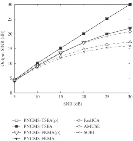
Part B: Performance Comparison for Sources with Different Power Spectra. In this part, we compare the proposed algo-rithms with the SOS-based algoalgo-rithms, namely the AMUSE [2] and SOBI [1] algorithms, and the FastICA using kurtosis [11]. The mixing matrix A = A1 (P = 5,K = 4) was
used, and parameters (μ1,μ2,μ3,μ4)= (1, 0.4, 0.3, 0.2) were
set for bi[n], i = 1, 2, 3, 4, so that the four source signals would have different power spectra. Both of the AMUSE and SOBI algorithms design theP×Ksource separation matrix (demixing matrix)V =[v1,v2,. . .,vK] =WTUusing SOS,
30 25
20 15
10 5
SNR (dB) PNCMS-TSEA(p)
PNCMS-TSEA NCMS-TSEA
PNCMS-FKMA(p) PNCMS-FKMA NCMS-FKMA 0
5 10 15 20 25 30
Output
SINR
(dB)
Figure2: Performance comparison results of Part A (output SINR versus SNR) forA=A1.
30 25
20 15
10 5
SNR (dB) PNCMS-TSEA(p)
PNCMS-TSEA NCMS-TSEA
PNCMS-FKMA(p) PNCMS-FKMA NCMS-FKMA 0
5 10 15 20 25 30 35
Output
SINR
(dB)
Figure3: Performance comparison results of Part A (output SINR versus SNR) forA=A2.
whereWis theK×Pprewhitening matrix as presented in step (P1) in the proposed PNCMS-TSEA andUis aK×K
unitary matrix. All the sources are extracted simultaneously without involving temporal processing as follows:
s[n]=VTx[n]=UTWx[n]=UTz[n], (28) where z[n] = Wx[n] is the prewhitened data vector. The unitary matrix Uobtained by the AMUSE is through eigen decomposition of the correlation matrix Rz[τ] =
the AMUSE and with (τ1,τ2,τ3) = (1, 2, 3) for the SOBI
algorithm.
Figure 4 shows the simulation results (output SINR
versus SNR). It can be seen that all the observations about the performance of the proposed algorithms from Figures2 and3also apply toFigure 4. One can also observe from this figure that the proposed PNCMS-TSEA(p) () and PNCMS-TSEA () perform best (with highest Output SINR) while the proposed PNCMS-FKMA(p) () and PNCMS-FKMA ( ) algorithms perform second, and all of them exhibit superior performance over the AMUSE () and SOBI (×) algorithms. Moreover, the proposed PNCMS-FKMA ( ) and the FastICA () exhibit similar performance since both the PNCMS-FKMA and the FastICA [11] are NCMS kurtosis maximization algorithms with prewhitening processing per-formed prior to source extraction, except that the former employs the FKMA while the latter employs a gradient search algorithm (which may not be very computationally efficient) in source extraction.
Part C: Comparison of Computational Complexity and Pro-cessing Latency. In this part of simulations, we demon-strate the computational complexity improvements of the PTSEA/PFKMA over the existing NCMS-TSEA/NCMS-FKMA as well as the processing latency reduc-tion of the PNCMS-TSEA(p)/PNCMS-FKMA(p). For the simulation using mixing matrixA = A1 (P = 5,K = 4)
andA = A2 (P = 8,K = 4), the parameters μi in bi[n], i = 1,. . ., 4 were set to (μ1,μ2,μ3,μ4) = (1, 0.4, 0.3, 0.2),
while for the simulation using the mixing matrix A = A3
(P =8,K =6) the parametersμiinbi[n],i=1,. . ., 6 were set to (μ1,μ2,μ3,μ4,μ5,μ6)=(1, 0.8, 0.6, 0.4, 0.3, 0.2). Again,
all the simulation results in this part were obtained over 100 simulation trials.
Case A (number of iterations per source versus SNR). In the case, we calculated the average number of iterations (spent by FKMA) in extracting a single source signal spent by the NCMS-TSEA/NCMS-FKMA and the PNCMS-TSEA/PNCMS-FKMA. Figures 5(a) and 5(b) show the simulation results (average number of iterations per source versus SNR) for mixing matrices A = A1 and A = A2,
respectively. One can observe from these two figures that the computational complexity (in terms of the average number of iterations per source) of the proposed PNCMS-TSEA () is smaller than that of the NCMS-TSEA () and their com-putational complexity differences forA=A2are much larger
than those forA =A1. Furthermore, the source extraction
involved in the proposed PNCMS-TSEA was performed with prewhitened data of dimensionK = 4 while that involved in the NCMS-TSEA was performed with the original data of dimension P = 5 for the case of A = A1 and P = 8
for the case ofA = A2 indicating that their computational
complexity differences are substantial. These observations also apply to the computational complexity comparison between the PNCMS-FKMA () and the NCMS-FKMA (). To show the effectiveness of the parallel source extraction structure of the PNCMS-TSEA(p)/PNCMS-FKMA(p) about
30 25
20 15
10 5
SNR (dB) PNCMS-TSEA(p)
PNCMS-TSEA PNCMS-FKMA(p) PNCMS-FKMA
FastICA AMUSE SOBI 0
5 10 15 20 25 30
Output
SINR
(dB)
Figure4: Performance comparison results of Part B (output SINR versus SNR) forA=A1.
processing latency reduction, we, respectively, calculated their average number of stages and the average total process-ing latency defined as
Average total processing latency= 1
100
100
q=1
Fq
=1
I(q), (29)
where Fqis the total number of stages required in trialqand I(q)stands for the maximum number of iterations (spent in extracting one source) among thek() parallel TSEA/FKMA modules in (F4a) plus that in (F4c). For the PNCMS-TSEA/PNCMS-FKMA, the average processing latency was simply the total number of iterations spent in extracting all the source signals averaged over 100 independent runs.
Case B(average number of stages versus SNR). The simu-lation results for the average number of stages spent by the proposed BSS algorithms are presented in Figure 6(a) for A = A1 and in Figure 6(b) forA = A3, respectively. One
can observe from these two figures that the average number of stages of the proposed PNCMS-TSEA(p) () for the case ofA= A1is less than 2 and that for the case ofA= A3is
less than 3 in contrast to the 4 stages and 6 stages required by the NCMS-TSEA () forA=A1andA=A3, respectively.
These observations also apply to the comparison between the PNCMS-FKMA(p) () and the NCMS-FKMA ().
Case C (average processing latency versus SNR). Figures 7(a) and 7(b) show the simulation results of the average processing latency (defined in (29)) for mixing matricesA=
A1andA =A3, respectively. It can be observed from these
30 25
20 15
10 5
SNR (dB) NCMS-TSEA
PNCMS-TSEA
NCMS-FKMA PNCMS-FKMA 0
10 20 30 40 50 60 70 80 90
A
ver
age
n
umb
er
o
f
it
er
at
ions
p
er
sour
ce
(a)
30 25
20 15
10 5
SNR (dB) NCMS-TSEA
PNCMS-TSEA
NCMS-FKMA PNCMS-FKMA 0
10 20 30 40 50 60 70 80 90 100
A
ver
age
n
umb
er
o
f
it
er
at
ions
p
er
sour
ce
(b)
Figure 5: Complexity comparison results of Case A in Part C
(number of iterations per source versus SNR): (a)A=A1and (b) A=A2.
the proposed PNCMS-TSEA(p) (•) can be further reduced. Compared to the PNCMS-TSEA, the PNCMS-TSEA(p) has around 44% reduction (e.g., from around 225 iterations down to 125 iterations for SNR=5 dB) in the average total processing latency forA=A1, while around 33% reduction
(e.g., from around 450 iterations down to 310 iterations for SNR = 5 dB) forA = A3. The PNCMS-FKMA(p) (◦)
provides around 25% reduction in both cases compared to the PNCMS-FKMA ().
6. Conclusion
By incorporating the prewhitening processing (which has been widely used for noise reduction and dimension reduc-tion) into the existing NCMS-TSEA and NCMS-FKMA, we
30 25
20 15
10 5
SNR (dB) NCMS-FKMA/TSEA PNCMS-TSEA(p)
PNCMS-FKMA(p) 1
1.5 2 2.5 3 3.5 4 4.5 5
Av
er
ag
e
n
u
m
b
er
o
f
st
ag
es
(a)
30 25
20 15
10 5
SNR (dB) NCMS-FKMA/TSEA PNCMS-TSEA(p)
PNCMS-FKMA(p) 2
3 4 5 6 7 8
Av
er
ag
e
n
u
m
b
er
o
f
st
ag
es
(b)
Figure 6: Complexity comparison results of Case B in Part C
(average number of stages versus SNR): (a)A=A1and (b)A=A3.
30 25
20 15
10 5
SNR (dB) NCMS-TSEA
PNCMS-TSEA PNCMS-TSEA(p)
NCMS-FKMA PNCMS-FKMA PNCMS-FKMA(p) 0
50 100 150 200 250 300 350
A
ver
age
total
pr
oc
essing
lat
ency
(a)
30 25
20 15
10 5
SNR (dB) NCMS-TSEA
PNCMS-TSEA PNCMS-TSEA(p)
NCMS-FKMA PNCMS-FKMA PNCMS-FKMA(p) 0
100 200 300 400 500 600 700 800 900 1000
A
ver
age
total
pr
oc
essing
lat
ency
(b)
Figure7: Processing latency comparison results of Case C in Part C (average total processing latency versus SNR): (a)A=A1and (b) A=A3.
extraction structure at each stage. We have shown that parallel TSEA (FKMA) modules in the PNCMS-TSEA(p) (PNCMS-FKMA(p)) can extract most of the unknown source signals at each stage by simply using columns of an arbitraryK×Kunitary matrix as the initial conditions for the spatial filters of TSEA or FKMA. Our simulation results have demonstrated performance and computational complexity improvements by the PNCMS-TSEA and PNCMS-FKMA as well as substantial processing latency reduction by the PNCMS-TSEA(p) and PNCMS-FKMA(p). In particular, we empirically found that the TSEA(p) and PNCMS-FKMA(p) can extract all the source signals within 3 stages forK ≤ 10, meanwhile with more than 30% reduction in
the processing latency compared to the PNCMS-TSEA and PNCMS-FKMA, respectively.
Appendix
Proof ofLemma 1.With the assumptions (A1), (A2) and the noise-free assumption, it has been proven in [15] thatJ(e[n]) given by (5) attains maximum (either locally or globally regardless of whetherAis unitary or not) if and only if
e[n]=vTx[n]
=αksk[n] =vTAs[n]
(A.1)
=vTak
sk[n] + K
i=1,i /=k
vTai
si[n], (A.2)
whereαkis an unknown nonzero constant and the unknown integer k ∈ {1, 2,. . .,K}. Note that the columns ai, i = 1, 2,. . .,K, of the K ×K unitary matrix A form an orthonormal basis forR(A), that is,ai =1 andaTiaj =0 for alli /=j. Therefore, it can be inferred from (A.1) and (A.2) thatvTa
k=αkandvTai=0 for alli /=k, and therefore it must be true thatv=βkak. Sincev =1 we haveαk=βk= ±1.
Lemma 1then is proved.
Acknowledgments
This work was supported by the National Science Council under Grant NSC 96-2628-E-007-003-MY3. This work was partly presented at the Forty-First Asilomar Conference on Signals, Systems, and Computers, Pacific Grove, CA, USA, November 4–7, 2007.
References
[1] A. Belouchrani, K. Abed-Meraim, J.-F. Cardoso, and E. Moulines, “A blind source separation technique using second-order statistics,”IEEE Transactions on Signal Processing, vol. 45, no. 2, pp. 434–444, 1997.
[2] L. Tong, V. C. Soon, Y. F. Huang, and R. Liu, “AMUSE: a new blind identification algorithm,” inProceedings of the IEEE International Symposium on Circuits and Systems (ISCAS ’90), vol. 3, pp. 1784–1787, New Orleans, La, USA, May 1990. [3] C. Chang, Z. Ding, S. F. Yau, and F. H. Y. Chang, “A
matrix-pencil approach to blind separation of non-white sources in white noise,” inProceedings of IEEE International Conference on Acoustics, Speech and Signal Processing (ICASSP ’98), vol. 4, pp. 2485–2488, Seattle, Wash, USA, May 1998.
[4] P. Comon, “Independent component analysis, a new concept?”
Signal Processing, vol. 36, no. 3, pp. 287–314, 1994.
[5] A. Hyv¨arinen, J. Karhunen, and E. Oja,Independent Compo-nent Analysis, John Wiley & Sons, New York, NY, USA, 2001. [6] L. Tong, R.-W. Liu, V. C. Soon, and Y.-F. Huang,
“Inde-terminacy and identifiability of blind identification,” IEEE Transactions on Circuits and Systems, vol. 38, no. 5, pp. 499– 509, 1991.
[8] C. L. Nikias and A. P. Petropulu, Higher-Order Spectral Analysis: A Nonlinear Signal Processing Framework, Prentice-Hall, Englewood Cliffs, NJ, USA, 1993.
[9] J.-F. Cardoso, “Source separation using higher order moments,” inProceedingsof IEEE International Conference on Acoustics, Speech and Signal Processing (ICASSP ’89), vol. 4, pp. 2109–2112, Glasgow, UK, May 1989.
[10] R. Mart´ın-Clemente, J. I. Acha, and C. G. Puntonet, “Eigende-composition of self-tuned cumulant-matrices for blind source separation,”Signal Processing, vol. 84, no. 7, pp. 1201–1211, 2004.
[11] A. Hyv¨arinen and E. Oja, “A fast fixed-point algorithm for independent component analysis,”Neural Computation, vol. 9, no. 7, pp. 1483–1492, 1997.
[12] Z. Ding, “A new algorithm for automatic beamforming,” in
Proceedings of the 25th Asilomar Conference on Signals, Systems, and Computers (ACSSC ’91), vol. 2, pp. 689–693, Pacific Grove, Calif, USA, November 1991.
[13] O. Shalvi and E. Weinstein, “Super-exponential methods for blind deconvolution,” IEEE Transactions on Information Theory, vol. 39, no. 2, pp. 504–519, 1993.
[14] Y. Inouye and K. Tanebe, “Super-exponential algorithms for multichannel blind deconvolution,”IEEE Transactions on Signal Processing, vol. 48, no. 3, pp. 881–888, 2000.
[15] Z. Ding and T. Nguyen, “Stationary points of a kurtosis max-imization algorithm for blind signal separation and antenna beamforming,”IEEE Transactions on Signal Processing, vol. 48, no. 6, pp. 1587–1596, 2000.
[16] C.-Y. Chi and C.-Y. Chen, “Blind beamforming and maximum ratio combining by kurtosis maximization for source separa-tion in multipath,” inProceedings of the 3rd IEEE Workshop on Signal Processing Advances for Wireless Communications (SPAWC ’01), pp. 243–246, Taoyuan, Taiwan, March 2001. [17] C.-Y. Chi, C.-Y. Chen, C.-H. Chen, and C.-C. Feng, “Batch
processing algorithms for blind equalization using higher-order statistics,”IEEE Signal Processing Magazine, vol. 20, no. 1, pp. 25–49, 2003.
[18] K. Yang, T. Ohira, Y. Zhang, and C.-Y. Chi, “Super-exponential blind adaptive beamforming,” IEEE Transactions on Signal Processing, vol. 52, no. 6, pp. 1549–1563, 2004.
[19] J.-F. Cardoso, “Infomax and maximum likelihood for blind source separation,”IEEE Signal Processing Letters, vol. 4, no. 4, pp. 112–114, 1997.
[20] K. Matsuoka and M. Kawamoto, “A neural net for blind separation of nonstationary signal sources,” in Proceedings of the IEEE International Conference on Neural Networks (ICNN ’94), vol. 1, pp. 221–226, Orlando, Fla, USA, June-July 1994.
[21] S. Choi and A. Cichocki, “Blind separation of nonstationary and temporally correlated sources from noisy mixtures,” in
Proceedings of the 10th IEEE Workshop on Neural Netwoks for Signal Processing (NNSP ’00), vol. 1, pp. 405–414, Sydney, Australia, December 2000.
[22] D.-T. Pham and J.-F. Cardoso, “Blind separation of instanta-neous mixtures of nonstationary sources,”IEEE Transactions on Signal Processing, vol. 49, no. 9, pp. 1837–1848, 2001. [23] J. Zhang, L. Wei, and Y. Wang, “Computational decomposition
of molecular signatures based on blind source separation of non-negative dependent sources with NMF,” inProceedings of the 13th IEEE Workshop on Neural Networks for Signal Pro-cessing (NNSP ’03), pp. 409–418, Toulouse, France, September 2003.
[24] C.-Y. Chi and C.-H. Peng, “Turbo source extraction algorithm and noncancellation source separation algorithms by kurtosis maximization,”IEEE Transactions on Signal Processing, vol. 54, no. 8, pp. 2929–2942, 2006.
[25] C.-Y. Chi, C.-C. Feng, C.-H. Chen, and C.-Y. Chen, Blind Equalization and System Identification, Springer, London, UK, 2006.