Volume 2007, Article ID 63560,10pages doi:10.1155/2007/63560
Research Article
Fast Time-Domain Edge-Diffraction Calculations for
Interactive Acoustic Simulations
Paul T. Calamia1, 2and U. Peter Svensson3
1Program in Architectural Acoustics, School of Architecture, Rensselaer Polytechnic Institute, Troy, NY 12180, USA
2Department of Computer Science, Princeton University, Princeton, NJ 08544, USA
3Acoustics Research Centre, Department of Electronics and Telecommunications, Norwegian University of
Science and Technology, NO-7491 Trondheim, Norway
Received 1 May 2006; Revised 20 September 2006; Accepted 16 October 2006
Recommended by Werner De Bruijn
The inclusion of edge diffraction has long been recognized as an improvement to geometrical-acoustics (GA) modeling techniques, particularly for acoustic simulations of complex environments that are represented as collections of finite-sized planar surfaces. One particular benefit of combining edge diffraction with GA components is that the resulting total sound field is continuous when an acoustic source or receiver crosses a specular-zone or shadow-zone boundary, despite the discontinuity experienced by the associated GA component. In interactive acoustic simulations which include only GA components, such discontinuities may be heard as clicks or other undesirable audible artifacts, and thus diffraction calculations are important for high perceptual quality as well as physical realism. While exact diffraction calculations are difficult to compute at interactive rates, approximate calculations are possible and sufficient for situations in which the ultimate goal is a perceptually plausible simulation rather than a numerically exact one. In this paper, we describe an edge-subdivision strategy that allows for fast time-domain edge-diffraction calculations with relatively low error when compared with results from a more numerically accurate solution. The tradeoffbetween computa-tion time and accuracy can be controlled with a number of parameters, allowing the user to choose the speed that is necessary and the error that is tolerable for a specific modeling scenario.
Copyright © 2007 P. T. Calamia and U. P. Svensson. This is an open access article distributed under the Creative Commons Attribution License, which permits unrestricted use, distribution, and reproduction in any medium, provided the original work is properly cited.
1. INTRODUCTION
Edge-diffraction impulse responses (IRs) are useful for acoustic simulations involving objects or environments com-prising faceted surfaces and have been applied to many problems in acoustics such as loudspeaker radiation [1], noise-barrier analysis [2], and room-acoustics modeling [3]. Diffraction calculations correct for the high-frequency approximation inherent in modeling techniques based on geometrical-acoustics (GA) assumptions, allow for the mod-eling of sound propagation around occluders and into shadow zones, and provide a smooth, continuous sound-field at specular-zone and shadow-zone boundaries when combined with GA components. All of these factors are im-portant to achieve perceptual realism when auralizing sound fields for virtual-acoustic simulations. When dynamic or in-teractive simulations are required, continuity of the sound field becomes particularly important. Moving sources or
receivers (i.e., listeners) may cross a zone boundary where the associated GA component (the direct sound or a specu-lar reflection) experiences a discontinuity as it abruptly en-ters or drops out of the impulse response due to the presence of an occluder or a reflecting surface. Such discontinuities may be heard as clicks or other undesirable audible artifacts if diffraction is not included in the simulated sound field.
assumptions about frequency or geometry involves the exact Biot-Tolstoy-Medwin (BTM) expression for diffraction from an infinite rigid wedge [7,8], which has been derived in a line-integral formulation for finite edges [9]. However, the computational complexity of this method has restricted its use to static scenarios and offline calculations for dynamic simulations.
In this paper, we describe a technique which allows for fast calculations of edge-diffraction impulse responses based on the BTM formulation presented by Svensson et al. in [9]. This formulation is given as an integral along the diff ract-ing edge, suggestract-ing an approach in which the edge can be subdivided into segments for processing. We use a hybrid approach in which each edge is subdivided into two types of segments: sample-aligned segments, each of which con-tributes to exactly one sample of the diffraction IR; and large evenly sized segments which contribute to multiple IR sam-ples. The former provide a high level of accuracy, but their boundaries are relatively slow to compute and must be up-dated when the source or receiver is moved. Therefore, we use them only for a small part of the edge which contributes a significant portion of the total diffracted energy to the early part of the IR. The latter segments introduce some error, but their boundaries are independent of the source and receiver positions and can be computed quickly in a preprocessing step for use with the IR tails. The subdivision process, and thus the tradeoffbetween computation time and accuracy, can be controlled with a number of parameters, allowing the user to choose the speed that is necessary and the error that is tolerable for a specific modeling scenario.
The remainder of this paper is organized as follows. Section 2discusses related work on diffraction calculations and acoustic modeling.Section 3contains a brief review of the diffraction formulation in [9] that we use as a basis for our method. Section 4describes an extension to the edge-subdivision strategy presented in [10] which we use in our system, andSection 5addresses the various parameters avail-able for adjusting the speed and accuracy of the diffraction calculations. Section 6 presents example calculations along with timing and accuracy data, andSection 7contains con-clusions and suggestions for future work.
2. RELATED WORK
Modeling for interactive acoustic simulations is typically done with one of three basic techniques: the image-source method [11,12], ray tracing [13], or beam tracing [14].1All three are based on geometrical-acoustics assumptions, and thus consider sound propagation only along straight ray-like paths. Such behavior is only correct at asymptotically high frequencies, but GA modeling techniques can provide high levels of accuracy and realism when the dimensions of the
1Other acoustic-modeling techniques such as the boundary element method, the finite element method, and various finite-difference schemes attempt to solve the wave equation numerically, but are generally too computationally intensive to allow for interactive calculations and are thus not considered further in this work.
reflecting surfaces are large relative to wavelength. For accu-rate modeling at low frequencies, with relatively small sur-faces, and/or in densely occluded environments, edge diff rac-tion must be taken into account.
While there are many techniques to calculate edge dif-fraction, two are applied most commonly to acoustic simula-tions of virtual environments. The first, a frequency-domain method, is the Uniform Theory of Diffraction [6], an exten-sion of the Geometrical Theory of Diffraction [15]. Because the UTD describes diffraction along ray-like paths, it is well suited for integration with GA modeling techniques. UTD-based diffraction can be calculated sufficiently quickly for use in interactive sound-field simulations. However, the UTD is a high-frequency approximation which assumes the diff ract-ing edge has infinite length, and is valid only for source and receiver locations which are far from the edge.
The UTD has been used in two interactive acoustic mod-eling systems that utilize beam tracing to find the GA com-ponents. The first, developed by Funkhouser et al. [4] and Tsingos et al. [16], uses a precomputed beam tree with its root at a fixed source location to identify areas in a 3D model which can be reached by direct, reflected, and/or diffracted sound. As a receiver is moved throughout the modeled en-vironment, the beam tree is used to identify valid propaga-tion paths from the source to the receiver locapropaga-tion rapidly, allowing for interactive modeling. For each diffracting edge in a valid path, UTD-based diffraction is calculated based on the shortest path through the edge. For reduced computation time (with a corresponding reduction in accuracy), diff rac-tion calcularac-tions can be limited to receivers in shadow zones. In the second system, developed by Antonacci et al. [5,17,18], visibility diagrams for all reflecting surfaces in a 2.5D model (i.e., arbitrarily placed vertical walls with hor-izontal floors and ceilings) are precomputed using a dual-space representation of the model’s geometry. These visibility diagrams allow for rapid construction of beam trees, which in turn allows for interactive modeling with a moving source as well as a moving receiver. UTD diffraction coefficients can be computed for each diffracted path, or can be interpolated from a small set of precomputed values for faster processing. The second common diffraction-calculation method us-es the Biot-Tolstoy-Medwin (BTM) solution, a time-domain formulation for diffraction from a rigid or pressure-release wedge [7,8,19]. In particular, the BTM-based expression de-rived by Svensson et al. in [9] has been used by a number of authors (e.g., see [3,20,21]) because it is formulated as a line integral along the diffracting edge and thus is well suited for use with finite edges, and because the BTM solution gives an exact solution for diffraction from a rigid (or pressure re-lease) wedge. Further details of the BTM formulation in [9] are provided inSection 3as it is the basis for our approxima-tion technique.
(specifically (2) below), use the FFT to find the diff rac-tion frequency response, and fit a warped infinite-impulse response filter to the smoothed diffraction magnitude re-sponse. While this method has been used in dynamic sound rendering with the DIVA system (see [20, 23, 24]), the diffraction calculations must be done offline in a prepro-cessing stage given the positions of the (moving) source and receiver over time. Interactive simulations are not possible with this approach due to the computation time needed to compute the diffraction IRs and construct the approxima-tion filters. In [25,26], de Rycker and Torres et al. approxi-mate edge diffraction in a somewhat similar fashion with fi-nite impulse-response (FIR) low-pass filters. However, their method was only tested with static source and receiver pairs, was not integrated into a GA modeling system, and did not provide a way to estimate the frequency-domain diff rac-tion response needed for the filter construcrac-tion without full impulse-response calculations.
Commercially available acoustic modeling tools such as CATT [27] and Odeon [28] simulate the effects of diff rac-tion on the reflecrac-tion and scattering from finite surfaces by adjusting the spectra of specular reflections and the fraction of energy that is scattered in nonspecular directions. How-ever, they ignore diffraction into shadow zones, do not cal-culate explicit diffraction impulse responses, and do not pro-vide interactive simulations. Tsingos and Gascuel [29,30] in-teractively simulate occlusion effects due to diffraction from objects between a source and receiver, but also do not calcu-late diffraction explicitly.
3. BTM EDGE DIFFRACTION
As mentioned above, our diffraction approximations are based on a line-integral formulation of the exact BTM so-lution as described in [9]. Consider a rigid wedge of finite length, a point source S, and a receiverR whose positions are given with edge-aligned cylindrical coordinates (rS,θS,zS)
and (rR,θR,zR), respectively, as shown inFigure 1. The source
signal is defined asq(t)=ρ0A(t)/4π, whereρ0is the density of air andA(t) is the volume acceleration of the point source. Such a source signal implies that the free-field impulse re-sponse of the source ish(τ)=δ(τ−d/c)/d, wheredis the distance from the source to the receiver andcis the speed of sound. Sound pressure can be calculated through the convo-lution integral
p(t)= ∞
0 h(τ)q(t−τ)dτ. (1)
The continuous-time edge-diffraction IR at the receiver is given in [9] as an integral over the edge positionz,
h(τ)= − ν 4π
4
i=1 z2
z1
δ
τ−m+l c
βi
mldz, (2)
whereν= π/θW is the wedge index,θW is the open wedge
angle,δis the Dirac delta function,mandlare the distances fromSandR, respectively, to a position on the edge, andc is the speed of sound. Thez-coordinate values of the edge
PR
R
l rR zR
θR zS
θW
z
θS
rS S
m
PS
Figure1: Wedge geometry and coordinate system. Locations are specified in cylindrical coordinates wherer is the radial distance from the edge,θis measured from one of the two wedge faces, and thez-axis is aligned with the edge.PSandPRare virtual half-planes that containSandR, respectively, and the edge.
endpoints are used for the integration limitsz1andz2. The functionsβiare
βi=
sinνϕi
cosh(νη)−cosνϕi
, (3)
where the anglesϕiare the four combinations ofπ±θS±θR
and the auxiliary functionηis
η=cosh−1
ml+z−zS
z−zR
rSrR .
(4)
The shortest path from the source to the receiver through the line that contains the edge goes through the so-called apex point on that line, and this apex point may or may not be contained within the physical edge. If it is, the onset time of the diffraction IR is determined by the path through the apex point. If it is not, the onset time is determined by the shorter of the two paths through the endpoints of the physi-cal edge.
The conversion of (2) into a discrete-time formulation, h(n), can be accomplished by subdividing the edge into seg-ments, and for each segment calculating the IR contribu-tion and distributing it among the appropriate time sam-ples. Numerical integration over each segment is generally straightforward, but the edge-diffraction IR expression is subject to an onset singularity when cosh(νη)=cos(νϕi)=1
as seen in (3). This singularity is addressed in [31], and an-alytical approximations are given for the first sample of the discrete-time IR,h(n0), which is the only sample affected.
4. EDGE-SUBDIVISION STRATEGIES
R
n2n1 n0 n1 n2
S
Boundaries for a 3-sample alignment zone Original even-segment boundaries (upper edge) Modified even-segment boundaries (lower edge)
Figure2: Unfolded 2D view of a source, receiver, and segmented edge. The upper edge is marked with the boundaries for a 3-sample alignment zone (samplesn0,n1, andn2) in black and the origi-nal even-segment boundaries in red. The lower edge (SandRnot shown) is marked with the modified segment boundaries for the hybrid subdivision scheme in blue: even segments overlapping the alignment zone have been truncated at the edges of the zone, and those completely within the alignment zone have been discarded. The apex point is marked with an “x.”
subdivision into evenly sized segments [9, 10].2 A third method, which is a hybrid of these two, was proposed in a simpler form in [10], and the remainder of this paper de-scribes the implementation and the evaluation of a more ro-bust form of that method.
4.1. Subdivision into sample-aligned segments
Sample-aligned segments correspond to portions of an edge which lie between intersections with two confocal ellipsoids (seeFigure 2). The foci of the ellipsoids are the source and receiver locations, and the lengths of the axes are deter-mined by the distancesc(n±0.5)/FS, where FS is the
sam-pling frequency andnis the sample index. With such bound-aries, each segment contributes to exactly one sample of the discrete-time diffraction IR, which can be written
h(n)= − ν 4π
4
i=1 zn,2
zn,1
βi
mldz. (5)
2Medwin et al. [19] and Clay and Kinney [32] also address the conversion of a continuous-time diffraction IR to a discrete-time diffraction IR, al-though they do so using a form of (2) given as an integral over time so they do not formulate the conversion as an edge-subdivision problem.
Calculation of the integration limits zn,1 andzn,2 involves finding the roots of a quadratic equation and is described in [31].
Sample-aligned segments are advantageous for many rea-sons. First, despite the low-pass filtering implied by the area sampling in (5), the spectrum of the discrete-time IR can be made to match that of the exact continuous-time IR up to a chosen frequency by using a sufficiently high sampling rate.3 Second, this method can be used easily with the analytical approximations for samplen0in [31] to avoid the onset sin-gularity because the boundaries corresponding to that sam-ple are given explicitly. Finally, the per-segment processing is straightforward: each segment’s contribution is calculated using either numerical integration or the analytical approxi-mation, and the result is added to the corresponding sample of the IR.
Sample-aligned segments unfortunately are not practi-cal for interactive simulations because of the associated com-putational demands. The segment-boundary calculations are time consuming, the boundaries must be recalculated when the source or receiver is moved, and high sampling frequen-cies often result in high segment counts.
4.2. Subdivision into evenly sized segments
Evenly sized segments for an edge of lengthLare generated by choosing a maximum lengthΔz, and subdividing the edge intoksegments of lengthlwherek = L/Δzandl =L/k. The segment-boundary values are easily calculated and are independent of the source and receiver locations; thus they can be calculated once in a simple preprocessing step. How-ever, excessively large values oflorΔzcan introduce signifi-cant errors in the resulting IR, while small values may result in a prohibitively large number of segments to process. Per-segment processing is somewhat more complicated than with sample-aligned subdivision because each segment may con-tribute to multiple IR samples. For each segment, the group of corresponding samples must be determined, and the to-tal segment contribution must be calculated and then spread appropriately across these samples. Finally, the boundaries corresponding to samplen0are not given explicitly, making it more difficult to avoid the onset singularity.
When using evenly sized segments that contribute to multiple IR samples, the amplitude valueAobtained by in-tegrating over the length of a segment must be distributed among the appropriate samples. The path lengths from the source to the receiver through the endpoints of a segment can be used to calculate the span of samples,Ssp, to which the
segment contributes, andAcan be distributed in a number of ways. The simplest approach is to evenly distributeAamong the samples, but this leads to a staircase effect in the IR. As described in [10], we apply a correction to the even distri-bution to achieve a linear approximation of the local slope
5670 5675 5680 5685 5690 Time (samples)
1.3 1.35 1.4 1.45 1.5 1.55 1.6 1.65 1.7
10
5
A
m
plitude
(ar
bit
rar
y
u
nits)
Sample-aligned segments
Even segments without slope correction Even segments with slope correction
Figure3: Multi-sample distribution for evenly sized segments with and without the slope correction, which assumes the impulse re-sponse has a locally linear decay.
of the IR. An example of the multi-sample distribution with and without the slope correction can be seen inFigure 3.
4.3. Hybrid subdivision strategy
A hybrid subdivision strategy can be used to exploit some of the benefits of both sample-aligned and evenly sized seg-ments. With this method, a small number of sample-aligned segments is used to calculate the first N samples of the diffraction impulse response, and evenly sized segments are used to process the remainder of the edge. Any portion of an evenly sized segment that overlaps the alignment zone (i.e., would contribute to any of the firstN samples) is dis-carded. An example of hybrid subdivision with N = 3 is shown in Figure 2. If the source or receiver is moved, the boundaries for the firstNsegments must be recalculated and the alignment-zone overlap tests must be repeated, but this is far less time consuming than recalculating sample-aligned boundaries for the entire edge. This method was introduced in [10], but utilized only a one-sample alignment zone.
5. CALCULATION PARAMETERS
Given the hybrid subdivision method described above, our goal is to minimize the diffraction processing time while lim-iting the error in the calculations. Three parameters provide control over the accuracy and timing: the number of samples in the alignment zone; the size of the evenly sized segments; and the integration technique used to calculate the contribu-tion of each segment, which can be chosen independently for the alignment zone and the even segments.
5.1. Size of the alignment zone
Because diffraction impulse responses tend to have an im-pulsive onset followed by a rapidly decaying tail, the high-frequency response is governed by the early samples. The low-frequency response is determined by the total integral over the entire edge, but this value also is strongly depen-dent on the early part of the IR which has a high amplitude relative to that of the tail. Therefore, accurate computation of the early part of a diffraction IR is critical for an accurate reproduction of its broadband spectral content and thus its perceptual characteristics. Our implementation of the hybrid edge-subdivision scheme allows for an alignment zone of ar-bitrary size, although as described inSection 6the use of as few as 4 sample-aligned segments can be sufficient for results with low spectral error.
5.2. Segment size
The size of the even segments is given in terms of the max-imum number of IR samples,nS, to be spanned by any one
segment, and converted to a length using
Δz=nS·c
FS
, (6)
where cis the speed of sound and FS is the sampling
fre-quency. In practice, the actual sample span of most segments is well below the specified upper bound ofnS. A single value
ofΔzis used for all edges in a given modeling environment. As Δz increases, computation time decreases due to fewer calls of the integration function, and accuracy decreases be-cause each segment’s diffraction contribution must be dis-tributed over a larger span of samples, and the assumption of a locally linear slope over such a span becomes less valid.
5.3. Numerical integration technique
Our implementation provides a choice of three numerical tegration techniques: 5-point compound Simpson’s rule in-tegration with one step of Romberg extrapolation, standard 3-point Simpson’s rule integration, and 1-point midpoint in-tegration [33]. Because the integrand, βi/ml, includes one
hyperbolic and two standard trigonometric functions (see (3)), a reduction of the number of points at which it must be evaluated can lower the total processing time significantly for multi-edge environments, albeit with a corresponding re-duction in accuracy. Any of the three techniques can be cho-sen for the alignment zone and for the evenly sized segments independently. However, the relative importance of the early part of the diffraction IR suggests that combinations in which the integration technique for the alignment zone is equal to or more accurate than that for the evenly sized segments will yield the best results.
6. RESULTS
S2
S1 R1
R2
(a)
Figure4: Plan view of the panel array used to evaluate the diffrac-tion approximadiffrac-tion method. The array was located 5 m above sourcesS1andS2and receiversR1andR2.
panels described in [34], similar to one which might be de-ployed over the stage in a concert hall or other performance space. The array comprises 35 infinitely thin 1.2 m by 1.2 m panels in a 5-by-7 grid with an inter-panel spacing of 0.5 m. 140 diffracting edges (4 for each panel) were evaluated for each calculation with the array positioned 5 m above two source/receiver pairs. The array and the source and receiver positions are shown in Figure 4. All calculations included first-order diffraction only; neither of the source/receiver pairs engendered a specular reflection from the array, and the direct sound and higher diffraction orders were omitted. Due to the absence of GA components, our testing scenarios are conservative in the sense that they overemphasize the need for accurate diffraction modeling.
All processing was done on a desktop computer with a 3.2 GHz Pentium 4 processor and 2 gigabytes of RAM, and all impulse responses were generated with a sampling rate of 96 kHz. All computation times are averages from 100 tri-als, and represent the time to compute all 140 diffraction IRs for the total panel-array response. For each of the two source/receiver pairs, the impulse response generated with sample-aligned segments and 5-point integration for all sam-ples was used as the baseline for all speed and accuracy eval-uations. Such calculations previously have been shown to agree quite well with measured data [35,36], so no compar-isons to measured data are included here.
For a conservative approximation of the audibility of the errors in the diffraction IRs, we calculated the diff rac-tion magnitude spectra, smoothed them with 1/10-octave filters, and compared them with the smoothed spectrum of the corresponding baseline case. Differences of less than 1 dB between 20 Hz and 20 kHz were assumed to be in-audible and thus acceptable for perceptual accuracy. Even though all diffracting edges were 1.2 m long, the individual impulse responses within the total response from the panel array ranged in size from 16 to 393 samples for the first source/receiver pair, and from 14 to 441 samples for the sec-ond source/receiver pair.
Using the hybrid method, we tested 180 combinations of the calculation parameters with each of the two source/
0 2 4 6 8 10 12 14 16 18 20
Processing time (ms) 0
2 4 6 8 10 12 14
1
/
10th-octa
ve
smoothed-spect
ru
m
er
ror
(dB
re.
1)
Source/receiver pair 1 Source/receiver pair 2
Figure5: Maximum error in the 1/10th-octave smoothed spectra below 20 kHz for various alignment-zone sizes (1 to 10 samples), segment sizes (40, 100, or 300 samples), and integration techniques (1-point, 3-point, or 5-point) using the hybrid method.
receiver pairs. These combinations included: variations in the size of the alignment zone from 1 to 10 samples; three sizes of evenly sized segments, specified as maximum sample spans of 40, 100, and 300 samples; and the three integration techniques used independently on the alignment zone and the evenly sized segments. Only combinations for which the alignment-zone integration technique was equal to, or more accurate than, that for the evenly sized segments were used. For example, given an alignment zone of 5 samples, evenly sized segments limited to a span of no more than 100 sam-ples, and 3-point alignment-zone integration, only 3-point and 1-point integration were tested for the evenly sized seg-ments.
Table1: Parameters resulting in the 5 fastest processing times for eachS/Rpair with maximum error in the smoothed spectrum less than 1 dB. Data for the baseline calculations are also included for comparison as the last entry for eachS/Rpair.
S/R Zone Zone Segment Segment Proc. Max. Pair Size Integ. Size Integ. Time Error (Samples) (Samples) (ms) (dB) 1 4 1-point 100 1-point 3.67 .97 1 4 1-point 300 1-point 3.69 .94 1 5 1-point 100 1-point 3.86 .98 1 5 1-point 300 1-point 3.88 .96 1 2 3-point 100 1-point 4.01 .69
1 all 5-point N/A N/A 171.25 0
2 3 1-point 100 1-point 3.31 .68 2 4 1-point 100 1-point 3.50 .41 2 5 1-point 100 1-point 3.69 .38 2 6 1-point 100 1-point 3.88 .43 2 7 1-point 100 1-point 4.08 .32
2 all 5-point N/A N/A 137.51 0
0 2000 4000 6000 8000 10000 12000 14000 Number of integrand evaluations
2 4 6 8 10 12 14 16 18 20
P
roc
essing
time
(ms)
Source/receiver pair 1 Source/receiver pair 2
Figure6: Relationship between the processing time and number of evaluations of the diffraction integrand. Processing times are the same as those inFigure 5.
zone (N≈4 samples) to compute the onset of the diff rac-tion IRs allows for the use of simplified numerical integra-tion and moderately large evenly sized segments and thus rapid calculations with low error. Using the first entry for each source/receiver pair inTable 1, the processing time for S1 andR1 was reduced by a factor of 46.6 (from 171 ms to 3.67 ms) and that for S2 andR2 by a factor of 41.7 (from 138 ms to 3.31). As can be seen inFigure 6, the processing time for computing the total diffraction impulse response grows linearly with the number of evaluations of the diff rac-tion integrand. This further supports the use of a small
align-40 42 44 46 48 50 52 54 56
Time (ms) 4
2 0 2 4 6 8 10 12 14 16
10
3
A
m
plitude
(ar
bit
rar
y
u
nits)
Sample-aligned subdivision Hybrid subdivision
0 0.005 0.01 0.015
41.2 41.25 41.3 41.35 41.4
Figure7: Impulse responses for source positionS1and receiver po-sitionR1. The blue IR (shown in the main figure and the inset) is the baseline calculation using sample-aligned segments and 5-point in-tegration, and the red IR (inset only) is an approximation using hy-brid subdivision with the parameters specified in Line 1 ofTable 1.
0.0315 0.063 0.125 0.25 0.5 1 2 4 8 16 Frequency (kHz)
45 40 35 30 25 20 15 10
1
/
10th-octa
ve
smoothed
mag
nitude
(dB
re
.1
)
Sample-aligned subdivision Hybrid subdivision
Figure8: 1/10th-octave smoothed magnitude spectra for the im-pulse responses inFigure 7. SeeFigure 9for the difference between
the two.
ment zone, moderately large evenly sized segments, and sim-ple integration for rapid calculations.
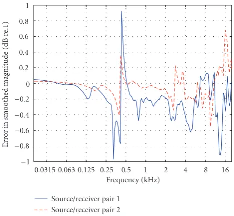
0.0315 0.063 0.125 0.25 0.5 1 2 4 8 16 Frequency (kHz)
1 0.8 0.6 0.4 0.2 0 0.2 0.4 0.6 0.8 1
Er
ro
r
in
smoothed
m
ag
nitude
(dB
re.1)
Source/receiver pair 1 Source/receiver pair 2
Figure9: Error in the smoothed spectrum for diffraction approxi-mations utilizing the geometry inFigure 4. The solid line is the er-ror for the example shown in Figures7and8usingS1andR1and the parameters in Line 1 ofTable 1. The dashed line is the error for an approximation usingS2andR2and the parameters in Line 7 of
Table 1.
following parameters (seeTable 1Line 1): an alignment zone of 4 samples, a maximum sample span for the even segments of 100 samples, and 1-point integration for the entire edge. Figure 7shows the total impulse response calculated for the panel array, and the inset contains a zoomed-in view of a portion of the IR where the hybrid method’s piecewise lin-ear approximation of the IR can be seen.Figure 8contains the smoothed magnitude spectra of the two IRs. The error (difference between the two spectra) is plotted inFigure 9, as is the error for an example calculation usingS2andR2with the parameters given in Line 7 ofTable 1. The maximum er-ror below 20 kHz occurs at approximately 325 Hz forS1and R1and at 13.05 kHz forS2andR2.
7. CONCLUSIONS
In this paper, we have presented an edge-subdivision strat-egy that allows for fast time-domain edge-diffraction cal-culations with low error. For a given scenario, each edge in a 3D model initially is subdivided into evenly sized seg-ments. As a source and/or receiver is moved in or around the model, the section of each edge which contributes to the first few samples of the edge-diffraction IR, which is de-pendent on the source and receiver positions, is subdivided into segments such that each one contributes to exactly one sample of the diffraction IR. Even segments overlapping this alignment zone are truncated at the edges of the zone, and those completely within the alignment zone are discarded. The diffraction integral is then evaluated for all remaining segments along the edge. Because the sample-aligned subdi-vision provides numerically accurate results with a high
com-putational cost, we generally restrict its use to the early por-tion of the IR which contains a significant percentage of the total diffracted energy and thus must be calculated accurately for a perceptually convincing simulation. However, a user is free to choose the size of the alignment zone, as well as the size of the evenly sized segments and the integration tech-nique(s) used to evaluate the two types of segments to opti-mize the speed-accuracy tradeofffor each modeling scenario. Tests on an array of rigid panels indicate that fast, low-error results can be obtained with an alignment zone of approx-imately 4 samples, even segments limited to a 100-sample span (with a sampling frequency of 96 kHz), and numerically simple midpoint integration for all segments. Our method can be combined easily with a geometrical-acoustics model-ing approach such as image-source modelmodel-ing or beam tracmodel-ing to provide rapid calculations of a smooth continuous sound field for interactive acoustic simulations.
This work suggests several avenues for future research. First, we would like to study the audibility of the errors in-troduced by the subdivision strategy. Our error criterion of 1 dB in the 1/10th-octave smoothed spectra is quite conser-vative and can likely be relaxed significantly when the diff rac-tion calcularac-tions are combined with GA components which typically dominate the sound field. However, listening tests could provide more definitive results, and possibly could provide guidelines for choosing subdivision parameter val-ues appropriate for different applications. The listening tests also could include comparisons to other fast diffraction ap-proximations, for example, those based on the UTD. While our method should provide higher accuracy, the perceptual benefits of that accuracy have yet to be established.
diffraction IRs where their amplitudes are maximal. Another approach could involve omitting edges for which the apex point is not included within the edge since the amplitude of the diffraction IR for such cases is small. Preliminary results for these forms of “diffraction culling” are presented in [39]. Finally, this subdivision scheme may aid in two addi-tional aspects of virtual acoustic simulations that include diffraction: visibility calculations and directional auraliza-tion. In regard to visibility, simulations of densely occluded environments require additional calculations to determine the portion(s) of each edge to which the source and receiver both have clear lines of sight. Approximate visibility could be computed by simply considering the visibility of the mid-point of each segment from the source and receiver. In regard to auralization of diffraction, Torres et al. [3] have suggested convolving each diffraction IR with the head-related impulse response specific to the direction of the least-time diffracted path. In some cases, however, an edge (from apex point to end point) may subtend an angle large enough such that a single direction of arrival for the entire IR is not sufficient for a perceptually accurate simulation. In such cases, the diff rac-tion IR could be auralized using paths through the midpoints of the segments (or a subset of segments) to allow the direc-tion of arrival to change over time.
ACKNOWLEDGMENTS
The authors would like to thank the Norway-America Asso-ciation, the Acoustics Research Centre project from the Re-search Council of Norway, and the National Science Founda-tion (Grant CCR-0093343) for partially funding this work, as well as the anonymous reviewers and the Associate Editor, Werner de Bruijn, for their helpful comments and sugges-tions.
REFERENCES
[1] J. Vanderkooy, “A simple theory of cabinet edge diffraction,”
Journal of the Audio Engineering Society, vol. 39, no. 12, pp.
923–933, 1991.
[2] P. Menounou and J. H. You, “Experimental study of the diffracted sound field around jagged edge noise barriers,”The
Journal of the Acoustical Society of America, vol. 116, no. 5, pp.
2843–2854, 2004.
[3] R. R. Torres, U. P. Svensson, and M. Kleiner, “Computation of edge diffraction for more accurate room acoustics auraliza-tion,”The Journal of the Acoustical Society of America, vol. 109, no. 2, pp. 600–610, 2001.
[4] T. Funkhouser, N. Tsingos, I. Carlbom, et al., “A beam tracing method for interactive architectural acoustics,”The Journal of
the Acoustical Society of America, vol. 115, no. 2, pp. 739–756,
2004.
[5] F. Antonacci, M. Foco, A. Sarti, and S. Tubaro, “Fast model-ing of acoustic reflections and diffraction in complex environ-ments using visibility diagrams,” inProceedings of 12th
Euro-pean Signal Processing Conference (EUSIPCO ’04), pp. 1773–
1776, Vienna, Austria, September 2004.
[6] R. G. Kouyoumjian and P. H. Pathak, “A uniform geometri-cal theory of diffraction for an edge in a perfectly conducting surface,”Proceedings of the IEEE, vol. 62, pp. 1448–1461, 1974.
[7] M. A. Biot and I. Tolstoy, “Formulation of wave propagation in infinite media by normal coordinates with an application to diffraction,”The Journal of the Acoustical Society of America, vol. 29, no. 3, pp. 381–391, 1957.
[8] H. Medwin, “Shadowing by finite noise barriers,”The Journal
of the Acoustical Society of America, vol. 69, no. 4, pp. 1060–
1064, 1981.
[9] U. P. Svensson, R. I. Fred, and J. Vanderkooy, “An analytic sec-ondary source model of edge diffraction impulse responses,”
The Journal of the Acoustical Society of America, vol. 106, no. 5,
pp. 2331–2344, 1999.
[10] P. T. Calamia and U. P. Svensson, “Edge subdivision for fast diffraction calculations,” inProceedings of IEEE Workshop on
Applications of Signal Processing to Audio and Acoustics, pp.
187–190, New Paltz, NY, USA, October 2005.
[11] J. B. Allen and D. A. Berkley, “Image method for efficiently simulating small-room acoustics,”The Journal of the Acoustical
Society of America, vol. 65, no. 4, pp. 943–950, 1979.
[12] J. Borish, “Extension of the image model to arbitrary polyhe-dra,”The Journal of the Acoustical Society of America, vol. 75, no. 6, pp. 1827–1836, 1984.
[13] A. Krokstad, S. Strøm, and S. Sørsdal, “Calculating the acous-tical room response by the use of a ray tracing technique,”
Jour-nal of Sound and Vibration, vol. 8, no. 1, pp. 118–125, 1968.
[14] T. Funkhouser, I. Carlbom, G. Elko, G. Pingali, M. Sondhi, and J. West, “A beam tracing approach to acoustic modeling for interactive virtual environments,” inProceedings of the 25th Annual Conference on Computer Graphics and Interactive
Tech-niques (SIGGRAPH ’98), pp. 21–32, Orlando, Fla, USA, July
1998.
[15] J. B. Keller, “Geometrical theory of diffraction,”Journal of the
Optical Society of America, vol. 52, no. 2, pp. 116–130, 1962.
[16] N. Tsingos, T. Funkhouser, A. Ngan, and I. Carlbom, “Model-ing acoustics in virtual environments us“Model-ing the uniform the-ory of diffraction,” inProceedings of the 28th Annual Confer-ence on Computer Graphics and Interactive Techniques
(SIG-GRAPH ’01), pp. 545–552, Los Angeles, Calif, USA, August
2001.
[17] F. Antonacci, M. Foco, A. Sarti, and S. Tubaro, “Accurate and fast audio-realistic rendering of sounds in virtual envi-ronments,” inProceedings of 6th IEEE Workshop on
Multime-dia Signal Processing, pp. 271–274, Siena, Italy,
September-October 2004.
[18] F. Antonacci, M. Foco, A. Sarti, and S. Tubaro, “Real time modeling of acoustic propagation in complex environments,”
inProceedings of 7th International Conference on Digital Audio
Effects (DAFx ’04), pp. 274–279, Naples, Italy, October 2004.
[19] H. Medwin, E. Childs, and G. M. Jebsen, “Impulse studies of double diffraction: a discrete Huygens interpretation,”The
Journal of the Acoustical Society of America, vol. 72, no. 3, pp.
1005–1013, 1982.
[20] V. Pulkki, T. Lokki, and L. Savioja, “Implementation and vi-sualization of edge diffraction with image-source method,”
inProceedings of 112th Audio Engineering Society Convention,
Munich, Germany, May 2002.
[21] P. T. Calamia, U. P. Svensson, and T. Funkhouser, “Integration of edge-diffraction calculations and geometrical-acoustics modeling,” inProceedings of Forum Acusticum, pp. 2499–2504, Budapest, Hungary, August 2005.
Acoustics and Sound Reinforcement, pp. 166–172, St. Peters-burg, Russia, June 2002.
[23] L. Savioja, J. Huopaniemi, T. Lokki, and R. V¨a¨an¨anen, “Cre-ating interactive virtual acoustic environments,”Journal of the
Audio Engineering Society, vol. 47, no. 9, pp. 675–705, 1999.
[24] L. Savioja, J. Huopaniemi, and T. Lokki, “Auralization ap-plying the parametric room acoustic modeling technique-the DIVA auralization system,” in Proceedings of the 8th
Inter-national Conference on Auditory Display, Kyoto, Japan, July
2002.
[25] N. de Rycker, “Theoretical and numerical study of sound diffraction-application to room acoustics auralization,” Rap-port de Stage D’Option Scientifique, `Ecole Polytechnique, Paris, France, 2002.
[26] R. Torres, N. de Rycker, and M. Kleiner, “Edge diffraction and surface scattering in concert halls: physical and perceptual as-pects,”Journal of Temporal Design in Architecture and the
En-vironment, vol. 4, pp. 52–58, 2004.
[27] B.-I. Dalenb¨ack,CATT-Acoustic v8 Manual,http://www.catt.se/. [28] C. L. Christensen, ODEON Room Acoustics Program ver. 8
Manual,http://www.odeon.dk.
[29] N. Tsingos and J.-D. Gascuel, “Soundtracks for computer an-imation: sound rendering in dynamic environments with oc-clusions,” inProceedings of the Conference on Graphics Inter-face, pp. 9–16, Kelowna, British Columbia, Canada, May 1997. [30] N. Tsingos and J.-D. Gascuel, “Fast rendering of sound occlu-sion and diffraction effects for virtual acoustic environments,”
inProceedings of the Audio Engineering Society 104th
Conven-tion, Amsterdam, The Netherlands, May 1998, preprint no. 4699.
[31] U. P. Svensson and P. T. Calamia, “Edge-diffraction impulse responses near specular-zone and shadow-zone boundaries,”
Acta Acustica united with Acustica, vol. 92, no. 4, pp. 501–512,
2006.
[32] C. S. Clay and W. A. Kinney, “Numerical computations of time-domain diffractions from wedges and reflections from facets,”The Journal of the Acoustical Society of America, vol. 83, no. 6, pp. 2126–2133, 1988.
[33] P. J. Davis and P. Rabinowitz,Methods of Numerical Integra-tion, Academic Press, New York, NY, USA, 2nd edition, 1984. [34] R. Torres,Studies of edge diffraction and scattering: applications
to room acoustics and auralization, Ph.D. thesis, Chalmers
Uni-versity of Technology, G¨oteborg, Sweden, 2000.
[35] T. Lokki and V. Pulkki, “Measurement and theoretical valida-tion of diffracvalida-tion from a single edge,” inProceedings of the
18th International Congress on Acoustics (ICA ’04), vol. 2, pp.
929–932, Kyoto, Japan, April 2004.
[36] A. Løvstad and U. P. Svensson, “Diffracted sound field from an orchestra pit,”Acoustical Science and Technology, vol. 26, no. 2, pp. 237–239, 2005.
[37] A. M. J. Davis and R. W. Scharstein, “The complete extension of the Biot-Tolstoy solution to the density contrast wedge with sample calculations,”The Journal of the Acoustical Society of
America, vol. 101, no. 4, pp. 1821–1835, 1997.
[38] J. C. Novarini and R. S. Keiffer, “Impulse response of a density contrast wedge: practical implementation and some aspects of its diffracted component,”Applied Acoustics, vol. 58, no. 2, pp. 195–210, 1999.
[39] U. P. Svensson and P. T. Calamia, “The use of edge diffraction in computational room acoustics,”The Journal of the
Acousti-cal Society of America, vol. 120, p. 2998, 2006, (A).
Paul T. Calamia is an Assistant Professor in the Graduate Program in Architectural Acoustics in the School of Architecture at Rensselaer Polytechnic Institute in Troy, NY. He earned a B.S. degree in mathematics from Duke University (1992), and an M.S. degree in electrical engineering in the Engi-neering Acoustics Program at the University of Texas at Austin (1998). He is currently in the process of completing a Ph.D. degree in
computer science at Princeton University, and he spent one year as a guest Ph.D. student with the Acoustics Group at the Norwegian University of Science and Technology in Trondheim. Between de-grees, he spent two years working as an Acoustical Engineer with Wyle Laboratories in Arlington, VA, and four years working as an Acoustics Consultant with Kirkegaard Associates in Chicago, IL. He is an Active Member of the Acoustical Society of America and its Technical Committee on Architectural Acoustics. His research interests include computational room acoustics, interactive sound-field simulations, edge-diffraction modeling, and spatial audio ren-dering.
U. Peter Svensson received his M.S. de-gree (Eng. Phys.) in 1987 and his Ph.D. degree in 1994, both from Chalmers Uni-versity of Technology, Gothenburg, Swe-den. He has held postdoctoral positions at Chalmers University, University of Water-loo, Ontario, Canada, and Kobe University, Japan. Since 1999, he has been a Professor in electroacoustics at NTNU in Trondheim. His research interests are auralization and