R E S E A R C H
Open Access
Robust reconstruction algorithm for compressed
sensing in Gaussian noise environment using
orthogonal matching pursuit with partially known
support and random subsampling
Parichat Sermwuthisarn
1, Supatana Auethavekiat
1*, Duangrat Gansawat
2and Vorapoj Patanavijit
3Abstract
The compressed signal in compressed sensing (CS) may be corrupted by noise during transmission. The effect of Gaussian noise can be reduced by averaging, hence a robust reconstruction method using compressed signal ensemble from one compressed signal is proposed. The compressed signal is subsampled forLtimes to create the ensemble ofLcompressed signals. Orthogonal matching pursuit with partially known support (OMP-PKS) is applied to each signal in the ensemble to reconstructLnoisy outputs. TheLnoisy outputs are then averaged for
denoising. The proposed method in this article is designed for CS reconstruction of image signal. The performance of our proposed method was compared with basis pursuit denoising, Lorentzian-based iterative hard thresholding, OMP-PKS and distributed compressed sensing using simultaneously orthogonal matching pursuit. The experimental results of 42 standard test images showed that our proposed method yielded higher peak signal-to-noise ratio at low measurement rate and better visual quality in all cases.
Keywords:compressed sensing (CS), orthogonal matching pursuit (OMP), distributed compressed sensing, model-based method
1. Introduction
Compressed sensing (CS) is a sampling paradigm that provides the signal compression at a rate significantly below the Nyquist rate [1-3]. It is based on that a sparse or compressible signal can be represented by the fewer number of bases than the one required by Nyquist theo-rem, when it is mapped to the space with bases incoher-ent to the bases of the sparse space. The incoherincoher-ent bases are called the measurement vectors. CS has a wide range of applications including radar imaging [4], DNA microarrays [5], image reconstruction and compression [6-14], etc.
There are three steps in CS: (1) the construction of a sparse signal, (2) the compression of a sparse signal, and (3) the reconstruction of the compressed signal. The focus of this article is the CS reconstruction of image data. The reconstruction problem aims to find the spar-sest signal which produces the compressed signal
(known as the compressed measurement signal). It can be written as the optimization problem as follows:
arg min
s s0s.t.y=s, (1)
where sand y are the sparse and the compressed
measurement signals, respectively;is the random mea-surement matrix having sampled meamea-surement vectors (known as random measurement vectors) as its column vectors ands0is the ℓ0 norm ofs. One of the ways to constructis as follows:
(1) Define the square matrix,, as the matrix having measurement vectors as its column vectors.
(2) Randomly remove the rows into make the row dimension ofequal to the one of.
(3) Settoafter row removal. (4) Normalize every column in
* Correspondence: [email protected]
Full list of author information is available at the end of the article
tion. In the greedy approach [19,20], the heuristic rule is used in place of ℓ1 optimization. One of the popular heuristic rules is that the non-zero components ofs cor-respond to the coefficients of the random measurement vectors having the high correlation to y. The examples of greedy algorithm are OMP [19], regularized OMP (ROMP) [20], etc. The greedy approach has the benefit of fast reconstruction.
The reconstruction of the noisy compressed measure-ment signals requires the relaxation of they−s con-straint. Most algorithms provide the acceptable bound
for the error between y and s [17-26]. The error
bound is created based on the noise characteristic such as bounded noise, Gaussian noise, finite variance noise, etc. The authors in [17] show that it is possible to use BP and OMP to reconstruct the noisy signals, if the conditions of the sufficient sparsity and the structure of the overcompleted system are met. The sufficient condi-tions of the error bound in basis pursuit denoising (BPDN) for successful reconstruction in the presence of Gaussian noise is discussed in [21]. In [22], the Danzig selector is used as the reconstruction technique. ℓ∞
norm is used in place ofℓ2 norm. The authors of [23] propose using weighted myriad estimator in the com-pression step and Lorentzian norm constraint in place ofℓ2 norm minimization in the reconstruction step. It is shown that the algorithm in [23] is applicable for recon-struction in the environment corrupted by either Gaus-sian or impulsive noise.
OMP is robust to the small Gaussian noise inydue to its ℓ2 optimization during parameter estimation. ROMP [20,26] and compressed sensing matching pursuit (CoSaMP) [24,26] have the stability guarantee as theℓ 1-minimization method and provide the speed as greedy algorithm. In [25], the authors used the mutual coher-ence of the matrix to analyze the performance of BPDN, OMP, and iterative hard thresholding (ITH) whenywas corrupted by Gaussian noise. The equivalent of cost function in BPDN was solved through ITH in [27]. ITH gives faster computation than BPDN but requires very sparse signal. In [28], the reconstruction by Lorentzian norm [23] is achieved by ITH and the algorithm is called Lorentzian-based ITH (LITH). LITH is not only
faster reconstruction.
Distributed compressed sensing (DCS) [33,35,36] is developed for reconstructing the signals from two or more statistically dependent data sources. Multiple sen-sors measure signals which are sparse in some bases. There is correlation between sensors. DCS exploits both intra and inter signal correlation structures and rests on the joint sparsity (the concept of the sparsity of the intra signal). The creators of DCS claim that a result from separate sensors is the same when the joint spar-sity is used in the reconstruction. Simultaneously OMP (SOMP) is applied to reconstruct the distributed com-pressed signals. DCS-SOMP provides fast computation and robustness. However, in case of the noisy y, the noise may lead to incorrect basis selection. In DCS-SOMP reconstruction, if the incorrect basis selection occurs, the incorrect basis will appear in every recon-struction, leading to error that cannot be reduced by averaging method.
In this article, the reconstruction method for Gaussian noise corrupted y is proposed. It utilizes the fact that image signal can be reconstructed from parts of y, instead of an entire y. It creates the member in the ensemble of sampled yby randomly subsamplingy. The reconstruction is applied to reconstruct each member in the ensemble. We hypothesize that all randomly
sub-sampled y are corrupted with the noise of the same
mean and variance; therefore, we can remove the effect of Gaussian noise by averaging the reconstruction results of the signals in the ensemble. The reconstruc-tion is achieved by OMP with partially known support (OMP-PKS) [34]. Our proposed method differs from DCS in that it requires only one yas the input. It is simple and requires no complex parameter adjustment.
2. Background 2.1 Compressed sensing
wherekis the number of the non-zero entries of sparse signal. Most natural signal can be made sparse by apply-ing orthogonal transforms such as wavelet transform, Fast Fourier transform, discrete cosine transform. This step is represented as
s=Tx, (2)
wherex is anN-dimensional non-sparse signal;sis a weighted N-dimensional vector (sparse signal with k
nonzero elements), andis an N×Northogonal basis matrix.
The second step is compression. In this step, the ran-dom measurement matrix is applied to the sparse signal according to the following equation.
y=s=Tx, (3)
whereis an M×N random measurement matrix
(M<N). Ifis an identity matrix,sis equivalent tox. Without loss of generality, is defined as an identity matrix in this article.Mis the number of measurements (the row dimension ofy) sufficient for high probability of successful reconstruction and is defined by
M≥Cμ2(,)k logN, (4)
for some positive constantC. μ(,)is the coher-ence betweenand, and defined by
μ(,) =√Nmax
i,j
φi,ψj. (5)
If the elements inandare correlated, the coher-ence is large. Otherwise, it is small. From linear algebra,
it is known that μ(,) ∈ 1,√N [2]. In the
mea-surement process, the error (due to hardware noise, transmission error, etc.) may occur. The error is added into the compressed measurement vector as follows.
y=s+e, (6)
whereeis anM-dimensional noise vector.
2.2 Reconstruction method
The successful reconstruction depends on the degree thatcomplies with RIP. RIP is defined as follows.
(1−δk)s22≤ s22≤(1 +δk)s22, (7)
where δkis the k-restricted isometry constant of a matrix. RIP is used to ensure that all subsets ofk col-umns taken fromare nearly orthogonal. It should be
noted thathas more column than rows; thus,
can-not be exactly orthogonal [2].
The reconstruction is the optimization problem to solve (1). In (2), when is an identity matrix,sis x. Equation (1) can be rewritten as (8). Equation (8) is the reconstruction problem used in this article.
arg min
x x0s.t.y=x. (8)
The reconstruction algorithms used in the experiment are BPDN, OMP-PKS, LITH, and DCS-SOMP. They are described in the following sections.
2.2.1 BPDN
BP [15,16] is one of the popularℓ1-minimization meth-ods. Theℓ0-norm in (8) is relaxed toℓ1-norm. It recon-structs the signal by solving the following problem.
arg min
x x1s.t.y=x. (9)
BPDN [21] is the relaxed version of BP and is used to reconstruct the noisy y. It reconstructs the signal by sol-ving the following optimization problem.
arg min
x x1 s.t.y−x2≤ε, (10)
whereεis the error bound.
BPDN is often solved by linear programming. It guar-antees a good reconstruction ifsatisfies RIP condition. However, it has the high computational cost as BP. 2.2.2. OMP-PKS
OMP-PKS [34] is adapted from the classical OMP [19]. It makes use of the sparse signal structure that some signals are more important than the others and should be set as non-zero components. It has the characteristic of OMP that the requirement of RIP is not as severe as BP’s [26]. It has a fast runtime but may fail to recon-struct the signal (lacks of stability). It has the benefit over the classical OMP as it can successfully reconstruct
yeven whenyis very small (very low measurement rate (M/N)). It is different from tree-based OMP (TOMP) [30] in that the subsequent bases selection of OMP-PKS does not consider the previously selected bases, while TOMP sequentially compares and selects the next good wavelet sub-tree and the group of related atoms in the wavelet tree.
In this article, sparse signal is in wavelet domain, where the signal in LL subband must be included for successful reconstruction. All components in LL sub-band are selected as non-zero components without test-ing for the correlation. The algorithm for OMP-PKS when the data are represented in wavelet domain is as follows.
Input:
• An M×N measurement matrix,
k {λi}
Procedure:
Phase 1: Basis preselection (initial step)
(a) Select every bases in LL subband.
t=||
t=
t=
ϕγ1ϕγ2...ϕγt .
(b) Solve the least squared problem to obtain the new reconstructed signal, zt.
zt = arg min
z y−tz2
(c) Calculate the new approximation,at, and find the residual (error, rt).atis the projection of y on the space spanned byt.
at=tzt rt= y - at.
Phase 2: Reconstruction by OMP
(a) Incrementtby one, and terminate ift>k. (b) Find the index,λt, of the measurement basis,ϕj, that has the highest correlation to the residual in the previous iteration (rt−1).
λt= arg max
j=[1,N],j∈/ t−1
rt−1,ϕj.
If the maximum occurs for multiple bases, select one deterministically.
(c) Augment the index set and the matrix of the selected basis.
t= t−1∪ {λt}and
t=
t−1 ϕλt .
at=tzt rt=y−at
(f) Go to step (a)
The reconstructed sparse signal, xˆ, has indexes of
non-zero components listed in k. The value of the
kth component of xˆ equals to the λjth component of zt. The termination criterion can be changed fromt>k to thatrt−1is less than the predefined threshold.
2.2.3. LITH
LITH [34] was proposed to reconstruct signals in the presence of Gaussian and impulsive noise. It differs from ITH in the usage of Lorentzian norm instead ofℓ2 norm. It reconstructs the signal according to the follow-ing function.
arg min
x y−xLL2,αs.t.x0 ≤k (11)
where uLL2,α is Lorentzian norm (LLqnorm withq (tail parameter) = 2) ofuand defined as follows.
uLL2,α= log
1 + 1
2 u
α
2
, (12)
whereαis a scale parameter. The algorithm for LITH is as follows.
Input:
•An M×Nmeasurement matrix,
•TheM-dimensional compressed measurement sig-nal,y
•The number of non-zero entries in the sparse sig-nal,k.
Output:
•The reconstructed signal,x.
(a) Setx(0)to zero vector andt to 0.
(b) At each iteration, x(t+ 1)was computed by
x(t+ 1) =Hk(x(t)) +μg(t)),
whereHk(a)is the nonlinear operator where thek lar-gest components ina are kept but the remaining com-ponents are set to zero.μis the step size. In this article,
gis defined as follows.
g(t) =TWt(y−x(t)).
Wt is an M×N diagonal matrix. The diagonal ele-ment in Wtis defined as
Wt(i,i) = α 2
α2+ (y
i−Tix(t))
2,i= 1, ....,M.
The step size is set as
μ(t) =
gk(t)(t)2
2
W1/2t k(t)gk(t)(t) 2
2
.
In case that y−x(t+ 1)LL
2,α >y−x(t)LL2,α, μ(t) is set to0.5μ(t).
(c) Terminate when the difference betweenxand y is less than or equal to the predefined error.
LITH is the fast and robust algorithm but it faces the same problem as ITH. It requires that either xmust be very sparse or y must be very large (high measurement rate). It is faster than OMP but with less stability. 2.2.4. DCS-SOMP
DCS uses the concept of joint sparsity, which is the sparsity of every signal in the ensemble. It is used under
the environment that there are a number of y whose
original signals (x) are related. It has three models: sparse common component with innovations, common sparse support, and non sparse common component with sparse innovations [31,33]. In this article, the com-mon sparse support model is used. SOMP [31,36] is proposed as the reconstruction algorithm. SOMP is adapted from OMP.
DCS-SOMP searches for the solution that contains max-imum energy in the signal ensemble. Given that the ensemble ofyis{yi};i= 1, 2, ...,L. The basis selection
cri-terion in DCS-SOMP is changed from
λt= arg max
j=[1,N],j∈/ t−1
rt−1,ϕj
to λt= arg max j=[1,N],j∈/ t−1
L
i=1ri,t−1,ϕi,j,
whereri,t−1is the residual ofyito the projection ofyion to the space spanned byt−1. The rest of the procedure remains the same as OMP. The indexes of non-zero com-ponents in the reconstructed xi(i= 1, 2, ...,L)are the
same, but the value of non-zero components may differ. It should be noted that whenLis equal to one, the DCS-SOMP is OMP.
3. Proposed method
This section addresses the problem of image reconstruc-tion from Gaussian noise corrupted y. The block pro-cessing is applied to reduce the computational cost. Block processing and the vectorization of the wavelet coefficients is described in Section 3.1. The proposed
reconstruction process from the ensemble of y is
explained in Section 3.2.
3.1 Block processing and the vectorization of the wavelet coefficients
In this article, the image is sparsified by the octave-tree discrete wavelet transform. Figure 1 shows an example of block processing and vectorization of the wavelet coeffi-cients. Figure 1a shows the structure of a wavelet trans-formed image. The LL3 subband is shown in red. Other subbands (LH, HL, and HH) in the third, the second, and the first level are shown in green, orange, and blue, respec-tively. The LL3subband is the most important subband, because it contains most of the energy in the image. Figure 1b shows the re-ordering of the wavelet coefficients. The coefficients are ordered such that the LL3 subband is located at the beginning of each row. The LL3subband is followed by the other subbands in the third, the second, and the first level.
The wavelet-domain image in Figure 1b is divided into blocks along its row as shown in Figure 1c. In Figure 1c, the image has eight rows and is divided into eight blocks. The signal can be made sparser by wavelet shrinkage thresholding [37]. All coefficients in LL3 sub-band are preserved. By using the wavelet shrinkage thresholding, we can set most coefficients in the other subbands to zero with little distinct visual degradation. Each row in Figure 1c is considered as the sparse signal for our study.
3.2. Reconstruction
The reconstruction method is divided into three stages: the construction of the ensemble of y, the
reconstruc-tion by OMP-PKS, and data merging. 3.2.1. Construction of the ensemble ofy
Given that there areLdifferentpM-dimension signals in the ensemble of y. pis the ratio of the sampled signal’s size to the original size.pandLare predefined. Theith signal in the ensemble is denoted by yi. The algorithm for constructing yiis as follows.
Input:
•An M×Nmeasurement matrix,
•The M-dimensional compressed measurement sig-nal,y
•The dimension ofyi,β =pM.
Output:
•Theith signal in the ensemble,yi.
•The truncated measurement matrix for yi,i
Procedure:
(a) Create the set of β random integers,
R={r1,r2, ...,rβ}, having the following properties. For all j,l∈[1,β],rj∈[1,M]andrj=rlonly if j=l. (b) Construct yiby setting the jth component ofyi
to the rjth component ofyfor all j∈[1,β].
(c) Constructi, according to the following function.
For all j∈[1,β], set the jth row ofito therjth row of.
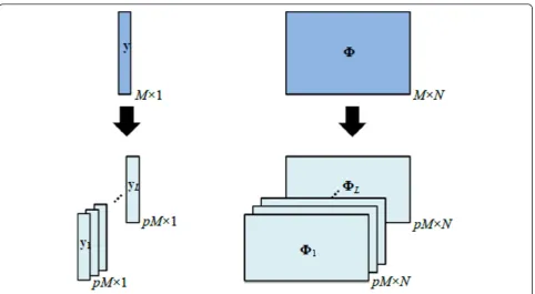
Figure 3 shows the result of applying the above proce-dure for Ltimes to create the ensemble ofLsampled signals. The total dimension of the ensemble is
pM×1×L. The ensemble is accompanied by L trun-cated measurement matrices. The size of the truntrun-cated
matrix is pM×N. Since all yi’s are the parts of the samey, their information is the same and they contain Gaussian noise of the same mean and the same var-iance. As long as the reconstruction does not use all sig-nals in the ensemble at once, it is safe to assume that reconstruction results from different yicontain different noise.
3.2.2. Reconstruction by OMP-PKS
The reconstruction of the proposed algorithm has the following requirements:
- the reconstruction of the signal at low measure-ment rate (M/N),
- fast reconstruction,
- independent reconstruction result for each signal in the ensemble.
The first requirement comes from the fact that the reconstruction is performed on the sampled signal which is smaller than y. The RIP is not always guaran-teed. The second requirement is necessary because the reconstruction must be performed Ltimes (Lis the number of the signal in the ensemble). The third requirement is the result of taking the information from only one signal. By combining every sampled signal, ori-ginal noisy y will be acquired. In the proposed algo-rithm, the denoising by averaging is possible when each
yi has the distinct reconstruction result from one another. Since each yi carries different set of the y’s components, its total noise is different. Consequently, the reconstruction on each yigives the result having dif-ferent noise corrupted to each pixel. The noise in each pixel can be reduced by averaging.
Even though the reconstruction is performed on the
ensemble of y as DCS, DCS-SOMP is not applicable,
be kept low (the first requirement) by including the model into the reconstruction. OMP-PKS [34] is chosen in this algorithm, because its requirement for
measurement rate is low. The experiment in [34] shows that the requirement of OMP-PKS was lower than CoSaMP-PKS.
OMP-PKS is applied to every yiin the ensemble and formsLdifferent sparse signals (wavelet coefficient). At the end of this stage, there areLnoisy images.
3.2.3. Data merging
Lnoisy images at the end of the reconstruction process have noise that is similar to Gaussian noise (Figure 4). At the same position, the noise in different reconstructed images had distinctly different magnitude; consequently, it can be reduced by taking the average at each pixel. Because the average is not done in spatial domain, there-fore the loss in spatial resolution is low. The denoising in spatial domain can be done by using the conventional denoising algorithms such as the Gaussian smoothing model [38], the Yaroslavsky neighborhood filters and an elegant variant [39,40], the translation invariant wavelet thresholding [41], and the discrete universal denoiser [42].
4. Experimental results 4.1. Experiment setup
The proposed method, OMP-PKS+random subsampling (OMP-PKS+RS), was compared with BPDN, LITH, OMP-PKS, and DCS-SOMP. The performance compari-son was evaluated using 42 standard test images with the size of 256 × 256 (available at http://decsai.ugr.es/ cvg/dbimagenes/index.php) as depicted in Figure 5. Each image was transformed to the wavelet domain using db8. The measurement matrix is Hadamard matrix. Each wavelet image was divided into the block
of 1 × 256. The number of blocks was 256. The average sparsity rate (k/N) of blocks in an image was 0.1. Peak signal-to-noise ratio (PSNR) and visual inspection were used for performance evaluation. All PSNRs shown in the graph were average PSNRs.
Since the compression step in CS consists mostly of linear operations, Gaussian noise corrupting the signal in the earlier states is approximated as the Gaussian noise corrupting the compressed measurement vector. The state where the noise corrupted the image was not specified; therefore, we simply corrupted the compressed measurement vector by different level of Gaussian noise indicated by its variance (σ2).
The experiment consists of two parts: (1) the evalua-tion for the required parameters (Landp) of OMP-PKS +RS and DCS-SOMP in Section 4.2 and (2) the perfor-mance evaluation in Section 4.3.
4.2. Evaluation forLandp
Both OMP-PKS+RS and DCS-SOMP require the ensem-ble ofy. We randomly subsampledywith the algorithm described in Section 3.1 to create the ensemble. First, we investigated for the size of the ensemble (L) and the size of the signal in the ensemble for the optimum perfor-mance of OMP-PKS+RS and DCS-SOMP. The size of the signal in the ensemble was investigated in term of the ratio to the size ofy(p).
set to 0.4. The solid line and the dashed line show the PSNR of the reconstruction by DCS-SOMP and OMP-PKS+RS, respectively. Figure 6a-d shows the PSNR when the noise variance was 0.05, 0.1, 0.15, and 0.2, respectively. The figures clearly show that the best per-formance of OMP-PKS+RS was better than the one of DCS-SOMP in all cases.
The line in the graph of Figure 6 was shown in differ-ent color to represdiffer-entpthat was varied. The effect ofp
was more pronounced in OMP-PKS+RS than in DCS-SOMP. The maximum PSNR in OMP-PKS+RS was achieved whenp= 0.6in all cases, while the maximum PSNR in DCS-SOMP was achieved with different value
of p. When σ2 were 0.05, 0.1, 0.15, and 0.2, the
optimum pfor DCS-SOMP were 0.9, 0.6, 0.7, and 0.6, respectively. No trend could be established for optimum
pin DCS-SOMP.
The x-axis in Figure 6 represents L. When Lwas changed, the performance of DCS-SOMP was almost unchanged. On the other hand, the performance of
OMP-PKS+RS was better, when Lwas larger. When
then noise was higher, OMP-PKS+RS required larger L
to achieve the optimum performance. In order to achieve the best performance, OMP-PKS+RS required the largerLthan DCS-SOMP in all cases. In most cases, DCS-SOMP and OMP-PKS+RS had already converged
to their optimum performance at L= 6 and 31,
The optimumpandLat variousM/Nand various noise levels were summarized in Tables 1 and 2, respectively. In DCS-SOMP, the optimumpvaried from 0.6 to 0.9. Out of 20 cases shown in the table, the optimumpwas 0.7 in 10 cases. The result in Figure 6 indicated thatphad little effect to the PSNR, sopfor DCS-SOMP was set to 0.7 in Section 4.3. In OMP-PKS+RS, the optimumpvaried from 0.6 to 0.8, note that in most cases (16 out of 20 cases) the
optimumpwas 0.6. Even thoughpin OMP-PKS+RS had
more effect to the result’s PSNR than DCS-SOMP, it was found that the PSNR difference between the best case and
p= 0.6was less than 0.5 dB. Hence,pfor OMP-PKS+RS
was set to 0.6 in Section 4.3.
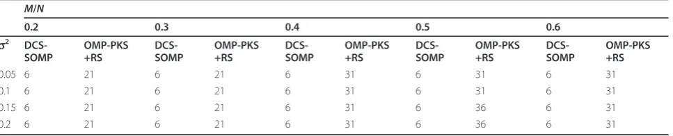
From Table 2 the optimum Lfor DCS-SOMP was
always equal to 6; thus,Lfor DCS-SOMP was set to 6 in Section 4.3. In OMP-PKS+RS, the optimumLvaried from 21 to 36. Out of 20 cases shown in the table, the optimum
Lwas 31 in 10 cases. The optimumLfor OMP-PKS+RS
was set to 31 in Section 4.3.
4.3. Performance evaluation
The performance of OMP-PKS+RS was compared with the ones of BPDN, LITH, OMP-PKS, and DCS-SOMP in this section. BPDN, LITH, and OMP-PKS used the single y to reconstruct the result, while OMP-PKS+RS
and DCS-SOMP used the ensemble of y. The error
bound of BPDN was set to σ2. The value ofa in LITH was set to the optimum value of 0.25 [28].
4.3.1. Evaluation by PSNR
Figure 7a-d shows the PSNR when σ2was set to 0.05, 0.1, 015, and 0.2, respectively. Different reconstruction methods are shown in different color. When M/N was higher, better reconstruction was achieved in all cases. However, the effect of the measurement rate to the per-formance of OMP-PKS+RS was lower than the other techniques.
Figure 7 also indicates that the proposed OMP-PKS +RS was the most effective reconstruction at small M/N
(< 0.4). WhenM/N= 0.4or higher, the PSNR acquired by the reconstruction from OMP-PKS+RS and
DCS-SOMP was approximately the same. At σ2= 0.05and
M/N= 0.6, all techniques achieved approximately the same PSNR. However, when the noise was increased, the reconstruction from the signal ensemble (OMP-PKS +RS and DCS-SOMP) was better than the performance of the reconstruction from one signal (BPDN, LITH, and OMP-PKS) in all cases but atM/N= 0.2.
It should be noted that even though LITH was designed for the reconstruction of noisy signal, its per-formance was the worst in almost all cases. This was due to its requirement of very sparse data (or very high
M/N). Its performance was still not converged at
M/N= 0.6; however,M/N could not be increased inde-finitely. The major benefit of CS is the capability to reconstruct the signal from small y, so the large M/N
will eliminate the CS benefit. For example, at the spar-sity rate of 0.1,M/N= 0.5would lead toy with the size of 50% of the original image size. Such large compressed
image could be achieved by conventional image com-pression techniques. Thus, it was rare that M/N could be increased to 0.5 or larger.
Since OMP-PKS+RS and OMP-PKS used the same reconstruction method, the PSNR difference between OMP-PKS+RS and OMP-PKS indicated the PSNR improvement by using the ensemble of y. The average PSNR improvement was more than 1 dB in allσ2. With the exception ofσ2= 0.05, the PSNR from OMP-PKS +RS at M/N= 0.2was higher than the one from OMP-PKS atM/N= 0.6. It indicated that by using the
ensem-ble of signal, OMP-PKS+RS required lower M/N to
achieve the same performance level of OMP-PKS. 4.3.2. Evaluation by visual inspection
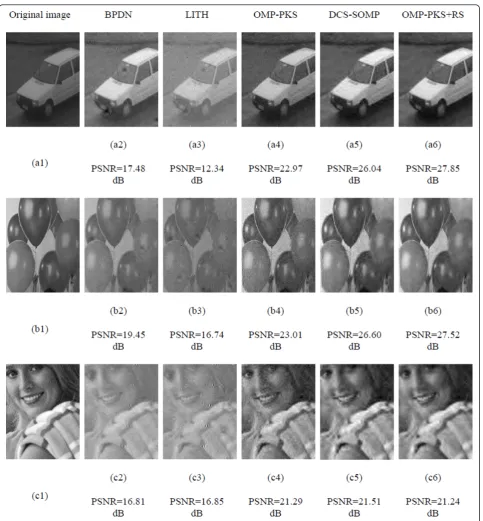
Images of Car, Pallons, and Elaine were used in this sec-tion. Car was selected because it contains the sharp edge. Pallons was selected because it has numbers of smooth surface. Elaine was selected because it contains a number of textures. Figure 8 shows the examples of reconstruction results when M/N= 0.4andσ2= 0.05. The original images are shown in the first column. The reconstruction results based on BPDN, LITH, OMP-PKS, DCS-SOMP, and OMP-PKS+RS are shown in the second, the third, the fourth, the fifth, and the sixth col-umns, respectively. BPDN and LITH failed to recon-struct some blocks as shown as dark dots (such as on the car’s windshield in Figures 8(a2-3), the rightmost balloon in Figures 8(b2-3)). Moreover, the results showed that OMP-PKS, DCS-SOMP, and OMP-PKS+RS successfully reconstructed every part. The smoothest reconstruction was acquired from the proposed OMP-PKS+RS. In all images, the change in the intensity
Table 2 The number ofLat which the converged PSNR was guaranteed
M/N
0.2 0.3 0.4 0.5 0.6
s2 DCS-SOMP OMP-PKS +RS DCS-SOMP OMP-PKS +RS DCS-SOMP OMP-PKS +RS DCS-SOMP OMP-PKS +RS DCS-SOMP OMP-PKS +RS
contrast was due to the normalization of the inverse wavelet transform.
The PSNR performance of the proposed OMP-PKS +RS and DCS-SOMP was very close; hence, further
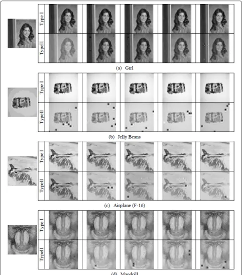
visual investigation is performed. Figures 9, 10, and 11 showed the examples of reconstruction based on OMP-PKS+RS and DCS-SOMP whenσ2= 0.05, 0.1, 0.15, and 0.2 and M/N≥0.4. The top and the bottom rows are Figure 7The average PSNR of reconstructed results whenyis corrupted by Gaussian noise with (a)σ2
=0.05, (b)σ2
the reconstruction based on DCS-SOMP and OMP-PKS +RS, respectively. Although DCS-SOMP gave higher PSNR, its result was noisy. The noise was reduced in the reconstruction based on OMP-PKS+RS. The edge was sharper and the uniform intensity regions were smoother. For example, atσ2
= 0.2andM/N= 0.6, the PSNR of the reconstructed Car based on DCS-SOMP
was 5.36 dB higher than the one based on OMP-PKS +RS. But as Figure 9 indicated, the car’s body in the top row was less smooth and the edge was more blurred. Similar examples could be found in Figures 10 and 11. Furthermore, DCS-SOMP failed to reconstruction some blocks (shown as dark dots), while OMP-PKS+RS suc-cessfully reconstructed every images.
4.3.3. Evaluation between OMP-PKS+RS and DCS-SOMP at optimum L and p
The performance of OMP-PKS+RS and DCS-SOMP at optimumLand pwas compared, in this section. M/N
dB higher PSNR at M/N= 0.2 and 0.3, respectively. DCS-SOMP started to have the higher PSNR when
M/Nwas set larger than 0.4. The trend was the same as the result in Section 4.3.1.
Figure 12 shows the reconstruction examples when L
OMP-PKS+RS, respectively. Even though the PSNRs of some images in the top row were higher, the images in the bottom row had sharper edge and smoother uniform regions. Noise was less distinct in the reconstruction
based on OMP-PKS+RS. The result followed the same trend as the result in Section 4.3.2.
Figure 12 was lower than Figures 9, 10, and 11. At σ2= 0.2, the PSNR of the reconstructed Car based on DCS-SOMP dropped from 24.61 dB (Figure 9) to 17.07 dB (Figure 12). The reconstructed image was also degraded visually. On the other hand, the reconstructed
Car based on OMP-PKS+RS at σ2= 0.1had 2.31 dB
lower PSNR but the visual quality was approximately the same. The PSNR and visual quality drop were also found in other images but with less degree (e.g., the reconstruction of Pallons based on DCS-SOMP at σ2= 0.2).
The PSNR drop was caused by the variance of the best pamong test images. The visual quality of the reconstruction based on OMP-PKS+RS was approxi-mately the same but the one based on DCS-SOMP dropped drastically in some cases. Consequently, it was possible to use onepfor every image in OMP-PKS+RS
but pmust be determined image by image in
DCS-SOMP.
From the comparison between OMP-PKS+RS and DCS-SOMP, it could be concluded that though OMP-PKS+RS produced the results with less PSNR than DCS-SOMP in some cases, the results had better visual quality. Furthermore, the parameter adjustment in OMP-PKS+RS was easier.
The reason behind the noise reduction was because the reconstruction based on OMP-PKS+RS produced different result for difference signal in the ensemble; therefore, the noise in each pixel could be reduced by averaging the intensity among signals in the ensemble. On the other hand, DCS-SOMP tried to find one result for every signal in the ensemble. Because the ensemble came from only one signal; hence, the noise was the same and the noise went directly to the result.
5. Conclusions
This article proposed the robust CS reconstruction algo-rithm for image with the presence of Gaussian noise. The proposed algorithm, OMP-PKS+RS, firstly applied
random subsampling to create the ensemble of L
sampled signals. Then OMP-PKS was used to recon-struct the signal. The Gaussian denoising was performed by averaging the image reconstruction of every signal in
the ensemble. The experiment shows that by using the ensemble of signal, the proposed algorithm improved the PSNR of the original OMP-PKS by at least 0.34 dB. Moreover, the proposed algorithm was efficient in removing the noise when the compression rate was high (small measurement rate). For future work, we plan to add the impulsive noise model into OMP-PKS+RS to develop the reconstruction algorithm that is robust to both impulsive and Gaussian noises.
Appendix 1: Computational costs of OMP, OMP-PKS, OMP-PKS+RS, and DCS-SOMP
The computational costs of OMP, OMP-PKS, OMP-PKS +RS, and DCS-SOMP are investigated. The variables are the same as in Sections 2 and 3. The number of multi-plication and the one of ℓ2 optimization are used to measure the computational cost. The computational cost of thetth iteration in the classic OMP is summar-ized in Table 4. The first||iterations in OMP are replaced by the basis preselection in OMP-PKS. The computational cost of the basis preselection is summar-ized in Table 5. The total computational costs of OMP and OMP-PKS for ak-sparse signal are as follows:
The number of multiplication in OMP =
k
t=1
(MN+M) (13)
The number of2optimization in OMP =
k
t=1
(2optimization fortvariables) (14)
The number of multiplication in OMP−PKS = k
t=||+1
(MN+M)+|| (15)
The number of2optimization in OMP−PKS =
k
t=||
(2optimization fortvariables) (16)
From (13) to (16), it can be concluded that OMP-PKS reduces the computational cost of OMP in two aspects.
(1) The number of multiplication of the first||th loops is reduced from(MN+M)||to||.
Figure 12Comparisons of reconstructed images by DCS-SOMP (top row) and OMP-PKS+RS (bottom row) whenpandLwas set according to Tables 1 and 2, respectively.M/Nwas set to 0.6.
Table 4 The computational cost of thetth iteration in OMP
Step The number of multiplication The number ofℓ2optimization
(1)λt= arg maxj∈/ t rt−1,ϕj. M(N-t+1)
-(2)at=Ftzt Mt
-(3)zt= arg minz||y-Ftzt-1||2 - ℓ2optimization fortvariables
In OMP-PKS+RS, the size of yiis reduced fromMto pM. The reconstruction is performedLtimes. Therefore,
the total computational time of OMP-PKS+RS is L
times the reconstruction of OMP-PKS, where M is
replaced bypM. In DCS-SOMP, the computational cost of thetth iteration is summarized in Table 6.
The total computational costs of OMP-PKS+RS and DCS-SOMP fork-sparse signal are as follows.
The number of multiplication in OMP−PKS + RS =Lp(MN+M)(k−) +|| (17)
The number of2optimization in OMP−PKS + RS =L
k
t=||
(2optimization fortvariables) (18)
The number of multiplication in DCS−SOMP =Lp(MN+M)k (19)
The number of2optimization in DCS - SOMP =L
k
t=1
(2optimization fortvariables) (20)
From (15) to (18), it can be concluded that the
com-putational cost of OMP-PKS+RS is approximately pL
times the cost of OMP-PKS. From (13), (14), (19) and (20), it can be concluded that the computational cost of
DCS-SOMP is pLtimes the cost of OMP. Since both
OMP-PKS+RS and DCS-SOMP reconstruct the ensem-ble of signals, their computational costs are higher than OMP and OMP-PKS.
From (17) to (20), it can be concluded that at the same Land p, the cost of OMP-PKS+RS is lower than DCS-SOMP because of the usage of OMP-PKS. How-ever, it was found that the optimum Land pin OMP-PKS+RS and DCS-SOMP were different. The product of
pLwas much higher in OMP-PKS+RS, so OMP-PKS+RS
had the highest computational cost. The effect of higher computing cost in OMP-PKS+RS can be reduced by parallel processing, because the reconstruction of each signal in OMP-PKS+RS can be done separately.
(1) λt= arg maxj=1,...,N l=1
rl,t−1,ϕj. LpM(N-t+1)
-(2)at=Ftzt LpMt
-(3)zt= arg minz||y-Ftzt-1||2 - L(ℓ2optimization fortvariables)
Total Lp(MN+M) L(ℓ2optimization fortvariables)
Table 7 The total computational cost of the reconstruction of ak-sparse signal by OMP, OMP-PKS, OMP-PKS+RS, and DCS-SOMP
Method The number of multiplication The number ofℓ2optimization
OMP (MN+M)k
k
t=1
(2optimization fortvariables)
OMP-PKS (MN+M)(k-|Γ|) + |Γ|
k
t=||
(2optimization fortvariables )
OMP-PKS+RS L[p(MN+M)(k- |Γ|) + |Γ|] L k
t=||
(2optimization fortvariables)
DCS-SOMP Lp[(MN+M)k] L
k
t=1
Table 7 summarizes the computational cost of the four methods, when they are applied to reconstruct a
k-sparse signal in Section 4.
Acknowledgements
The authors would like to thank the reviewers for their comments and suggestions. This research has financially been supported by the National Telecommunications Commission Fund (Grant No. PHD/006/2551 to P. Sermwuthisarn and S. Auethavekiat), the Telecommunications Research Industrial and Development Institute (TRIDI).
Competing interests
The authors declare that they have no competing interests.
Author details 1
Department of Electrical Engineering, Chulalongkorn University, Bangkok 10330, Thailand2National Electronics and Computer Technology Center,
Pathumthani, Thailand3Department of Electrical Engineering, Assumption University, Bangkok 10240, Thailand
Received: 2 April 2011 Accepted: 15 February 2012 Published: 15 February 2012
References
1. DL Donoho, Compressive sensing. IEEE Trans Inf Theory.52(4):1289–1306 (2006)
2. EJ Candes, MB Wakin, An introduction to compressive sampling. IEEE Signal Process Mag.25, 21-30 (2008)
3. EJ Candes, J Romberg, Sparsity and incoherence in compressive sampling. Inverse Problem.23(3):969–985 (2007). doi:10.1088/0266-5611/23/3/008 4. VM Patel, GR Easley, DM Healy, R Chellappa, Compressed synthetic aperture
radar. IEEE J Sel Topics Signal Process.4(2):244–254 (2010)
5. F Parvaresh, H Vikalo, S Misra, B Hassibi, Recovering sparse signal using measurement matrices in compressed DNA microarrays. IEEE J Sel Topics Signal Process.2(3):275–285 (2008)
6. G Shi, D Gao, D Liu, L Wang, High resolution image reconstruction: a new imager via movable random exposure. Proc ICIP, Cairo, Egypt. 1177–1180 (2009)
7. J Yang, Y Zhang, W Yin, A fast alternative direction method for TVL1-L2 signal reconstruction from partial fourier data. IEEE J Sel Topics Signal Proces.4(2):288–297 (2010)
8. RF Marcia, RM Willett, Compressive coded aperture superresoltion image reconstruction.Proc ICASSP. (Nevada, U.S.A., 2008), pp. 833–836
9. L Gan, Block compressed sensing of natural images.Proc DSP. (Wales, U.K., 2007), pp. 403–406
10. Y Yang, OC Au, L Fang, X Wen, W Tang, Perceptual compressive sensing for image signals.Proc ICME. (New York, U.S.A., 2009), pp. 89–92
11. TT Do, TD Tran, L Gan, Fast compressive sampling with structurally random matrices.Proc ICASSP. (Nevada, U.S.A., 2008), pp. 3369–3372
12. L Gan, TT Do, TD Tran, Fast compressive image using scrambled block hadamard ensemble.Proc EUSIPCO. (Lausanne, Switzerland, 2008) 13. S Mun, JE Fowler, Block compressed sensing of images using directional
transforms.Proc ICIP. (Cairo, Egypt, 2009), pp. 3021–3024
14. P Sermwuthisarn, S Auethavekiat, V Patanavijit, A fast image recovery using compressive sensing technique with block based orthogonal matching pursuit.Proc ISPACS. (Kanazawa, Japan, 2009), pp. 212–215
15. S Chen, DL Donoho, M Saunders, Atomic decomposition by basis pursuit. SIAM Rev.43(1):129–159 (2001). doi:10.1137/S003614450037906X 16. DL Donoho, M Elad, VN Temlyakov, Stable recovery of sparse overcomplete
representations in the presence of noise. IEEE Trans Inf Theory.52(1):6–18 (2006)
17. JA Tropp, Just relax: convex programming methods for identifying sparse signals in noise. IEEE Trans Inf Theory.52(3):1030–1051 (2006)
18. EJ Candes, J Romberg, T Tao, Stable signal recovery from incomplete and inaccurate measurements. Commun Pure Appl Math.59(8):1207–1223 (2006). doi:10.1002/cpa.20124
19. JA Tropp, AC Gilbert, Signal recovery from random measurements via orthogonal matching pursuit. IEEE Trans Inf Theory.53(12):4655–4666 (2007)
20. D Needell, R Vershynin, Uniform uncertaintity principle and signal recovery via regularized orthogonal matching pursuit. Found Comput Math.
9(3):317–334 (2009). doi:10.1007/s10208-008-9031-3
21. D Omidiran, MJ Wainwright, High-dimensional subset recovery in noise: sparsified measurements without loss of statistical efficiency, in Technical report 753. (Department of Statistics, UC Berkeley, U.S.A., 2008) 22. EJ Candès, T Tao, The dantzig selector: statistical estimation whenpis
much larger thann. Ann Stat.35(6):2313–2351 (2007). doi:10.1214/ 009053606000001523
23. RE Carrillo, KE Barner, TC Aysal, Robust sampling and reconstruction methods for sparse signals in the presence of impulsive noise. IEEE J Sel Topics Signal Proc.4(2):392–408 (2010)
24. D Needell, JA Tropp, CoSaMP: iterative signal recovery from incomplete and inaccurate samples. Appl Comput Harmonic Anal.26(3):301–321 (2008) 25. Z Ben-Haim, YC Eldar, M Elad, Coherence-based near-oracle performance
guarantees for sparse estimation under Gaussian noise. Proc ICASSP, Prague, Czech Republic. 3590–3593 (2010)
26. D Needell, Topics in compressed sensing.Ph.D. Dissertation, Math. (Univ. of California, Davis, 2009)
27. T Blumensath, ME Davies, Normalized iterative hard thresholding: guaranteed stability and performance. IEEE J Sel Topics Signal Process.
4(2):298–309 (2010)
28. RE Carrillo, KE Barner, Lorentzian based iterative hard thresholding for compressed sensing, inProc. IEEE ICASSP, Prague, Czech Republic. 3664–3667 (2011)
29. C La, MN Do, Signal reconstruction using sparse tree representation.Proc of SPIE Conf on Wavelet Applications in Signal and Image Proc. (San Diego, U.S. A, 2005), p. 5914
30. C La, MN Do, Tree-based orthogonal matching pursuit algorithm for signal reconstruction.Proc IEEE ICIP. (Georgia, U.S.A, 2006), pp. 1277–1280 31. MF Duarte, Compressed sensing for signal ensembles.Ph.D. Dissertation.
(Department of Electrical Engineering, Rice University, Houston, TX, 2009) 32. L He, L Carin, Exploiting strucrure in wavelet-based Baysian compressive
sensing. IEEE Trans Signal Process.57, 3488–3497 (2009)
33. D Baron, MB Wakin, MF Duarte, S Sarvotham, RG Baraniuk, Distributed compressed sensing.Technical Report, TREE-0612. (Rice University, Department of Electrical and Computer Engineering, Houston, TX, 2006) 34. RE Carrillo, LF Polania, KE Barner, Iterative algorithm for compressed sensing
with partially know support.Proc IEEE ICASSP. (Texas, U.S.A, 2010), pp. 3654–3657
35. M Xu, J Lu, K-cluster-values compressive sensing for imaging. EURASIP J Adv Signal Process (2011). doi:10.1186/1687-6180-2011-75
36. NV Aravind, K Abhinandan, VA Vineeth, DS Suman, Comparison of OMP and SOMP in the reconstruction of compressively sensed hyperspectral images.Proc IEEE ICCSP. (Hamirpur, India, 2011), pp. 188–192 37. D Donoho, De-noising by soft thresholding. IEEE Trans Inf Theory.
38(2):613–627 (1995)
38. F Catté, F Dibos, G Koepfler, A morphological scheme for mean curvature motion and applications to anisotropic diffusion and motion of level sets. SIAM J Numer Anal.32(6):1845–1909 (1995)
39. LP Yaroslavsky,Digital Picture Processing—An Introduction. (Springer Verlag, Berlin, Heidelberg, 1985)
40. L Yaroslavsky, M Eden,Fundamentals of Digital Optics. (Birkhauser, Boston, 1996)
41. RR Coifman, D Donoho,Translation-Invariant De-Noising, Wavelets and Statistics. (Springer Verlag, New York, 1995), pp. 125–150
42. E Ordentlich, G Seroussi, S Verdú, M Weinberger, T Weissman, A discrete universal denoiser and its application to binary image. in Proc IEEE ICIP, vol. 1. (Catalonia, Spain, 2003), pp. 117–120
doi:10.1186/1687-6180-2012-34