Volume 2007, Article ID 97961,17pages doi:10.1155/2007/97961
Research Article
A Survey of Architecture and Function of the Primary
Visual Cortex (V1)
Jeffrey Ng,1Anil A. Bharath,1and Li Zhaoping2
1Department of Bioengineering, Imperial College London, South Kensington Campus, London SW7 2AZ, UK
2Natural Intelligence Laboratory, Department of Psychology, University College London, Gower Street, London WC1E 6BT, UK
Received 1 December 2005; Revised 6 September 2006; Accepted 18 September 2006
Recommended by Gloria Menegaz
The largest visual area, known as the primary visual cortex or V1, has greatly contributed to the current understanding of mam-malian and human visual pathways and their role in visual perception. The initial discovery of orientation-sensitive neurons in V1, arranged according to a retinotopic mapping, suggested an analogy to its function as a low-level feature analyser. Subsequent discoveries of phase, spatial frequency, color, ocular origin, and direction-of-motion-sensitive neurons, arranged into overlapping maps, further lent support to the view that it performs a rich decomposition, similar to signal processing transforms, of the retinal output. Like the other cortical areas, V1 has a laminar organization with specialization for input from the relayed retinal afferents, output to the higher visual areas, and the segregation of the magno (motion) and parvo (form) pathways. Spatially lateral con-nections that exist between neurons of similar and varying properties have also been proposed to give rise to a computation of a bottom-up saliency map in V1. We provide a review of the selectivity of neurons in V1, laminar specialization and analogies to signal processing techniques, a model of V1 saliency computation, and higher-area feedback that may mediate perception.
Copyright © 2007 Jeffrey Ng et al. This is an open access article distributed under the Creative Commons Attribution License, which permits unrestricted use, distribution, and reproduction in any medium, provided the original work is properly cited.
1. INTRODUCTION
The primary visual cortex (V1) contains orientation-tuned neurons, arranged in a retinotopic map, which have become the hallmark of early cortical computation in the primate vi-sual system. Prior to the discovery of such neurons, the im-portant role of V1 in the human visual system was known in the early twentieth century through patients who suffered to-tal or partial loss of vision depending on the extent of damage to that area. The systematic correspondence between affected V1 area and regions of the field of view led Holmes [1] to deduce the retinotopic organization before the advent ofin vivoextra cellular recording. Since then, anatomical exami-nations have shown that the visual signals from the retina en-ter the visual cortex mainly through V1, which in turn feeds the higher visual areas [2,3]. The primary visual cortex thus plays an important role in visual perception in humans.
Attention was first drawn to the primary visual cortex by the discovery of edge and line “detector” neurons by Hubel and Wiesel in the late 1950s (see [4] for a review of their early work). These detector neurons are organized into smoothly changing maps of preferred orientation parallel to the sur-face of V1. Subsequently, V1 neurons selectively responding
to a variety of other stimuli, such as color, spatial frequency, eye of origin, motion, and even visual disparity between the two eyes were found. We provide a short review of key infor-mation about the function and architecture of V1 that may be used to build a blueprint of this crucial stage of the human visual system. We hope that this may assist efforts to reverse engineer the early human visual system or to transfer success-ful cortical strategies to computer vision and signal process-ing algorithms. Despite the large number of studies on V1, probably one of the most examined out of all the other visual areas, significant controversy still exists on the extent of the computation that V1 performs. For this purpose, our review will include mainly established experimental facts about V1 and we only briefly mention controversial areas. Owing to the huge amount of literature on V1, we selectively provide references for facts that cannot be found in standard text-books. Further details can be found in Winder’s review [5] and Olshausen and Field’s examination of what is still un-known about V1 [6]. In addition, we also present some more recent experimental data that have significant implications on the computational function of V1.
Ventricle Optic chiasm
Optic nerve Temporal retina
Upper quadrant
Visual fields
Macular area
Lower quadrant
Nasal retinae
Optic tract
Oculomotor Nerve Nuclei
Geniculate bodies Lateral Medial
Superior colliculus
Optic radiations
Visual cortex (area 17) Calcarine
sulcus
Left occipital cortex
P3D
Figure1: Illustration of the optic nerve, lateral geniculate nucleus (LGN) and V1 (area 17 in the figure), obtained from [7].
visual information are found in the visual cortex and are called V1, V2, V3, V4, V5/MT, MST, and so on. These cor-tical areas are interconnected with a high degree of regular-ity and precision [8]. The parallel connections from V1 to multiple higher cortical areas indicate that the human vi-sual system employs a hierarchical processing strategy [9], whereby the higher cortical areas are interconnected with a mixture of parallel and serial two-way connections. We first provide a brief overview of the human visual system (illus-trated inFigure 1). The retina contains an array of photore-ceptors, which samples the field of view, and ganglion cells which process the visual signal prior to transmission through the optic nerve. Even at the earliest stages of visual processing in the retina, anatomically distinct classes of neurons with different processing properties create two separate streams of information for motion and form. The optic nerve car-ries the visual signal to the thalamus where it is relayed by the lateral geniculate nucleus (LGN) to the primary visual cortex.
The neurons in the LGN and V1 maintain an ana-tomical and functional segregation of cells involved in the two streams, although some interconnections exist at the
boundaries of these anatomical regions in the LGN and V1. From V1, the two streams of information are separated into parallel neural connections to higher cortical areas, clearly demonstrating the existence of two parallel processing “path-ways” in the human visual system, termed dorsal and ventral pathways. The dorsal pathway consists of V1→V2→V5→
can be expressed as a linear combination of its inputs, which is analogous to the finite impulse response (FIR) of linear filters.
1.1. Anatomical structure
The primary visual cortex anatomically corresponds to Brod-mann’s area 17 and is visually identifiable as a distinctive stripe caused by the myelinated neurons in its fourth layer. For this reason, it is also called the striate cortex. The neu-rons of V1 are arranged into a thin slightly folded two-dimensional sheet with six separate layers. At an approximate surface area of 8 mm×6 mm and a thickness of 1.7 mm [12], V1 is the largest area in the visual cortex. The retinotopic or-ganization of the neurons indicates that V1 uses the spatial location of stimuli in the field of view to organize its analy-sis and this may have important implications on its function. Wandell [12] estimates the number of neurons in primate V1 to be at least 150 million which puts the ratio of V1 neurons to retinal ganglion output cells at 100 : 1. Even after allowing for the compression performed by the ganglion cells prior to transmission over the bandwidth-limited optic nerve, V1 produces more outputs than visual inputs leading to an over-complete representation of the visual field [13]. Each neuron makes in the order of thousands of short-range interconnec-tions with other neurons in V1 [12]. Neuron density and the number and destination of connections vary in the six layers of V1 (further details can be found in [14]).
2. SUBCORTICAL INPUTS
As in many other visual areas, the properties of neurons in V1 can be better understood by investigating the transforma-tions of the visual signals that occur in the earlier stages of the visual system. The major feedforward input to V1 con-sists of afferent nerve axons from the lateral geniculate nu-cleus which itself relays signals from the retina. A simplistic view of the function of these two early stages can be sum-marized as visual sensing, information encoding, and trans-mission from the frontal end of the skull to the visual cortex at the occipital (back) end. We provide a brief summary of these early subcortical computation and refer the reader to reviews such as [15,16] for more detail.
As an outgrowth of the brain, the retina contains a vari-ety of neurons, such as ganglion, amacrine, and bipolar cells among others, in addition to the light-sensing photorecep-tors. Incoming light across the visual fieldI(x) is sampled as a function of spatial location x by the photoreceptors and transformed to outputs O(x) by the retinal ganglion cells. The photoreceptors and ganglion cells vary in size and vi-sual properties according to their eccentricity from the cen-ter of the retina where the fovea is found. The family of so-called P-type ganglion cells, constituting about 85% of the total population, is predominantly found in the foveal re-gion and possesses high spatial resolution while responding sluggishly to changes. On the other hand, the periphery con-tains M-type cells which only make up 10% of ganglion cells
and which have poorer spatial resolution but higher tempo-ral resolution.
An analogy to the computation performed by the P-type ganglion cells in the fovea is a linear transform, O(x) =
K(x,x)I(x)dx, with adaptable dynamic range which de-pends on light levels and is adaptable over a time scale of less than 30 seconds. In daylight, the transform is similar to isotropic spatial bandpass filtering with a peak sensitiv-ity of around 3–5 cycles per visual degree. The kernel of the transformation can be approximated by a difference of two Gaussians, for example,K(x,x) ∝Ae−(x−x)2/(2σcenter)2
− Be−(x−x)2/(2σ2
surround), with space constantsσcenter< σsurroundand
weights A > B > 0 (orA < B < 0), which replicates the interaction between the central and surround subfields of receptive fields observed in extracellular recordings. In dim light, this transform changes to a lowpass filter or Gaussian-like smoothing filterK(x,x)∝e−(x−x)2/(2σ2)
. The adaptivity of the transform can be theoretically understood by assum-ing that the aim of the retinal computation is to transmit as much information as possible from the photoreceptors to the brain with limited information transmission capacity at the retinal output—the optic nerve composed of output fibers from the retinal ganglion cells [17,18]. The adaptation of the transform to light levels corresponds to different efficient codes for different input signal-to-noise levels. Applying the efficient coding principle to color coding leads to the red-center green-surround receptive fields of the neurons [19]. Hence, let the color input beI(x,c) for cone typec =red, green, blue, a cell with the red-centre-green-surround recep-tive field gives outputO∝ dxAe−(x−x)2/(2σ2
red)I(x, red)−
dxBe−(x−x)2/(2σgreen2 )I(x, green) with weightsA > B >0 (or
A < B <0), and spatial constantsσred< σgreen.
The segregation between the two main types of M and P ganglion cells output is preserved both in the optic nerve and in the lateral geniculate nucleus. The axons of P-type gan-glion cells project to the upper four layers of the LGN while the axons of the M-type cells project to the lower two layers. Allard [20] and Kaplan and Benardete [21] believe that M cells are responsible for the perception of movement while P cells help in the perception of form and color with their higher spatial acuity. Theoretically, the receptive fields of the M cells could be understood by assuming that their role is to extract input information as fast as possible (rather than as much as possible by P cells), given limited information trans-mission capacity [22].
3. TWO ASPECTS OF ORGANIZATION AND FUNCTIONS IN V1
Much of the initial investigations into the function and or-ganization of neurons in V1 were carried out by single-and multiple-cell extra cellular recording of their outputs to given, albeit simple, visual stimuli. While different families of neurons tuned to features such as orientation, spatial fre-quency, phase of symmetry, color, ocular origin, and direc-tion of modirec-tion were discovered and their responses to simple stimuli adequately characterized, the organization of these neurons on a larger scale and the lateral interactions between neurons in response to larger stimuli were less amenable to systematicin vivocharacterization. Fortunately, population recording techniques such a functional magnetic resonance imaging (fMRI) and optical imaging of the cortical surface have plugged the gap to reveal the organization of the neu-rons into overlapping retinotopic maps for different features [26]. Computational modelling techniques have also signif-icantly matured to propose plausible mechanisms for lateral interactions [27].
The huge interest in characterizing the functional proper-ties of neurons in V1 arises from the short distance in terms of synaptic connections, typically at least 4, from photore-ceptors in the retina and the compact spatial localization of the photoreceptors inputs contributing to the receptive fields of the neurons, which are usually no larger than 1 or 2 de-grees of visual angle. Hubel and Wiesel [28] identified three types of neurons: simple, complex, and hyper complex. A simple neuron performs a linear combination of its visual inputs and the population response of these neurons can be approximated by a linear filtering of the visual signal by their FIR masks, the signal processing analogy to biological recep-tive fields, followed by a nonlinear pointwise transform that is more or less monotonous with threshold and saturating behavior, that is, response=f(K(x,x)I(x)dx) with non-linearityf(·). According to the “energy” model [29], the out-put of two simple cells in quadrature (90◦phase difference) with a squaring nonlinear function f(·) can be summed to provide quasi-position-invariant responses of complex neu-rons within their receptive fields. Hypercomplex neuneu-rons re-spond to the end-stopping of lines. V1 contains a consequen-tial number of cell types with different classes of receptive fields and visual properties. The detailed and overcomplete representation of the visual field through the huge popula-tion of neuronal responses in V1 earned the latter its name “sorting office” of visual signals [30].
The presence of extensive lateral connections between neurons and the discovery of a class of inhibitory V1 in-terneurons [31] which do not directly receive visual input prompted a reexamination of the predominantly feedfor-ward role of neural circuits in V1, and in particular the nature of the receptive field. The classical Receptive Field (cRF) was measured by Hubel and Wiesel [28] with point light sources and bars. Such simple visual stimuli did not elicit any re-sponse beyond a certain distance from the center of the RF. However, the lateral connections and inhibitory interneu-rons hint at significant interactions between the computation
of nearby feedforward neurons. This interaction causes each cell’s response to be significantly influenced by stimuli out-side its classical receptive field in a region called its context or surround. Consequently, a neuron’s response can clearly signal global properties of input on a spatial scale much larger (e.g., of a typical visual object) than the classical recep-tive field [32–34]. Such a global property clearly has exciting computational implications. One could also view the classi-cal receptive field as arising from the feedforward processing of LGN inputs in V1, while the second contextual influence of stimuli outside the cRF as arising from the recurrent or lateral processing in V1. For clarity, we will first discuss the former before the latter.
3.1. Organization of individual cells in V1
V1 cells respond selectively to different input features [35], such as orientation, color, scale, spatial phase, direction of motion, and ocular origin. The selectivity of the neurons to specific features of visual stimuli, such as orientation, spatial phase, and scale, is achieved by the spatially defined linear function of the receptive fields. Selectivity to different types of stimuli such as colour and ocular origin is achieved by se-lecting the origin of the visual signals, for example, rod and cone photoreceptors on the retina, left or right eye. Living-stone and Hubel [36] found that V1 cells are usually simul-taneously tuned to more than one of these features, which is not surprising considering that they only perform a lin-ear combination of their visual inputs. For instance, simul-taneous tuning to both orientation and direction of motion is common. However, V1 neurons are usually more strongly tuned to one specific feature than others.
The retinotopic map of the primary visual cortex is a well-known feature. However, the correspondence between neuron location and the retinotopic location of their recep-tive fields is only evident over scales greater than 1.2 mm par-allel to the surface of V1 [37]. At smaller scales, neurons are organized by columns specializing in different stimuli. The selectivity of V1 neurons to different feature dimensions causes several overlapping maps to coexist parallel to the sur-face of V1 [37].
III
IV
Corticalmodule
Left eye Right
eye Left eye Right
eye
Ocular
dominanc
e columns Orientation columns
Blobs
Figure2: Illustration of a hypercolumn containing neurons selec-tive to orientation, ocular dominance, and color, obtained from [40].
A
B
6 5 4Cβ 4Cα 4B 4A 3 2 1 R L R L
Figure3: Ice cube model of the V1 area. The function and selec-tivity of cells remain more or less similar across the laminar layers and vary gradually along the surface. Cytochrome-oxidase staining reveals columns of colour sensitive cells in layer 2/3, obtained from [42].
over a range of about 3 octave of peak spatial frequencies and 20 orientations for a particular region of space. The discov-ery of columnar organizations prompted the emergence of the “ice cube” model of V1 (illustrated inFigure 3).
Freeman [41] performed a multiparameter study of the organization of neurons within columns of the primary vi-sual cortex of the cat. In particular, Freeman investigated whether pairs of adjacent neurons were related by common visual properties such as preferred orientation, spatial fre-quency, or spatial phase. Similarly to the original experi-ments of Hubel and Wiesel [28], Freeman found that pre-ferred orientation was the most similar in adjacent neurons. Spatial frequency was the next most common property, while the property that varied the most between adjacent neurons was spatial phase. This led Freeman to the hypothesise that V1 may use a strategy of pooling the response of neurons with different spatial phases to achieve phase invariance.
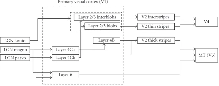
Figure 4 shows the connections from the LGN to V1, the intralaminar (intralayer) connections in V1, and the
projections from V1 to the upper areas of the cortex. V1 is divided into six different layers according to the relative den-sity of neurons, interconnections, and external connections from the LGN and to other visual areas [12]. Minor diff er-ences in the layers may cause further subdivisions. Layer 1 contains relatively few neurons and does not perform any major processing. The incoming LGN connections consist of two separate bundles originating from the magnocellu-lar and parvocellumagnocellu-lar layers and project to two neighboring but different subregions in sublayer 4C of V1 called layers 4Ca and 4Cb, respectively. The magnocellular pathway flows from layer 4Ca to 4B and then projects to the “thick stripes” of V2 and V5. The parvocellular pathway flows through layer 4Cb and then projects to the “blobs” and “interblobs” in lay-ers 2 and 3. The “thick stripes” of area V2 and the “blobs” and “interblobs” of layer 2/3 in V1 are qualitative descrip-tions of regions revealed by staining of cortical tissue with cytochrome oxidase. The latter is a metabolic enzyme which participates in the electron transport chain in the brain. The distinctive blobs contain cells that are color-selective and are tuned to both a broad range of orientations and to low spa-tial frequencies. In comparison, cells in the interblobs are the opposite with no color selectivity, high selectivity to par-ticular orientations and high spatial frequencies [36]. The presence of two types of regions in layer 2/3 and their sep-arate projections to different regions of V2 (also revealed by cytochrome-oxidase staining) prompted the view that the parvo “what” pathway specializes into two subpathways in V1: parvo-B deals exclusively with colour and Parvo-I deals with orientation and high acuity perception [30]. The dis-tinction between the properties of the cells in the blobs and the interblobs has been blurred by new research that revealed cells in the interblobs tuned to both color and orientation [38].
3.1.1. Orientation selectivity
Orientation-selective cells were the first type of feature de-tectors identified by Hubel and Wiesel [28] in V1. Three kinds of orientation-selective cells were actually found: sim-ple, complex, and hypercomplex. Simple cells respond selec-tively to lines or edges at particular orientations. Their pop-ulation response is obtained by linearly filtering the visual input by their RFs as in 2D signal processing. The filter can be approximated by a 2D Gabor function, for example, fil-ter∝ exp(−x2/2σ2
x −y2/2σy2) cos(2π f x+φ), illustrated in
Figure 5, which is oriented along the y-axis, with widthσx and lengthσy > σx, is tuned to optimal spatial frequency f and has a receptive field phase of symmetry φ (a phase of 0◦ or 90◦ makes the cell tuned to a bar or edge, resp.). The response of a simple cell is therefore also dependent on the spatial phaseφof the stimulus, that is, the precise location of the line with respect to the RF, with optimal response at
LGN konio
LGN magno LGN parvo
Layer 4Ca Layer 4Cb
Layer 6
Primary visual cortex (V1)
Layer 2/3 interblobs
Layer 2/3 blobs
Layer 4B
V2 interstripes
V2 thin stripes
V2 thick stripes
V4
MT (V5)
Figure4: Connections from LGN, interlayer connections and projections to other cortical areas. Note that layer 4C has been separated into 4Ca and 4Cb, adapted from [30,43].
a quarter of RF sizes [44]. This indicates a considerable de-gree of overlap of RFs. On the other hand, complex cells also selectively respond to lines or edges at particular orientations but their response is insensitive to the position of the line or edge within the RFs. A standard view [45] is that they receive inputs from simple cell subunits of different phases. They are abundant in layer 2/3 [30] and have also been reported in layer 6. A drifting sine grating stimulus would elicit a half-wave rectified modulation in the mean firing rate of a simple cell, and an approximately constant firing rate in a complex cell.
Although Hubel and Wiesel [35] initially discovered that V1 cells were tuned to the same orientation in a column, the degree of orientation selectivity was found to vary as one goes deeper into the column and the layers of V1 [46]. This is a property of the laminar specialization of V1. As the primary site of visual input from the LGN to V1, layer 4C appears to have broad orientation tuning. According to Ringach et al. [46] (who used grating stimulus to assess ori-entation selectivity), the neurons in layer 4C have the short-est average response time (45 milliseconds) in V1 to reti-nal stimulus. The longest average response time is found in layer 2 (70 milliseconds) where orientation tuning width (defined as half-width at 1/√2 height) is the narrowest at 20◦ on average, and layer 6 (65 milliseconds) which pos-sesses marginally sharper orientation tuning than layer 4C, whose tuning width is at 25◦ on average. The authors pro-pose that the increased delay in response time in layers 2 and 6 indicate significant lateral interactions between V1 cells to sharpen orientation selectivity. De Valois et al. [47] have ear-lier reported that orientation bandwidth in macaques at half-height of the maximum response ranges from 6◦to 360◦ (un-oriented) with a median near 40◦. There are also cells un-tuned or poorly un-tuned to orientation, they tend to be un-tuned to color and are in the CO blobs [36], which are associated with cells tuned to lower spatial frequencies [48].
Figure 6shows the arrangement of preferred orientation on a layer parallel to the surface of V1 in the cat. The pin-wheel arrangement (angularly varying) of selectivity around
central singularities is common in mammalian V1. The sharp breaks in this orderly arrangement, called fractures, corre-spond to important landmarks in the maps of other visual features such as the shift in eye of origin in ocular dominance maps.
3.1.2. Color selectivity
Three classes of cones (color photoreceptors) exist in the retina, selective to long (L), middle (M), and short (S) wave-lengths of light corresponding to red, green, and blue col-ors, respectively. As mentioned earlier, retinal ganglion cells and LGN cells combine color opponency (red-green and blue-yellow) and spatial opponency (center surround) in a red-center green-surround fashion [50], calledsingle oppo-nency. In V1, many cells are mainly tuned to either color or orientation [36], while some are tuned to both [38]. Cells tuned to color tend to have a double-opponency organiza-tion, for example, the center of the receptive field has the red-green opponency while the surround has the red-green-red op-ponency [36]. Using physiological and psychophysical data in his arguments, Lennie [9] proposes that a cortical neu-ron responds to multiple types of stimuli (e.g., binocular disparity, color, orientation, phase, etc.) and “pure” neurons which respond selectively to one type only of stimulus do not exist.
5 10 15 20 25 25
20 15 10 5
Cos Gabor
5 10 15 20 25 25
20 15 10 5
Sin Gabor
5 10 15 20 25 25
20 15 10 5
Envelope
(a)
5 10 15 20 25 25
20 15 10 5
Cos Gabor
5 10 15 20 25 25
20 15 10 5
Sin Gabor
5 10 15 20 25 25
20 15 10 5
Envelope
(b)
5 10 15 20 25 25
20 15 10 5
Sin: phase 0
5 10 15 20 25 25
20 15 10 5
Sin: phasex/6
5 10 15 20 25 25
20 15 10 5
Sin: phasex/3
5 10 15 20 25 25
20 15 10 5
Sin: phasex/2 cos!
(c)
5 10 15 20 25 25
20 15 10 5
Cos Gabor
5 10 15 20 25 25
20 15 10 5
Sin Gabor
5 10 15 20 25 25
20 15 10 5
Envelope
(d)
Figure5: Gabor patches, illustrating effects of parameter changes, notably angular selectivity (elongation), phase, and rotation. (a)σx=σy;
(b)σx=σy/2; (c) left to right, increasing phase shift and Gabor transformed from antisymmetric to symmetric.
color-selective neurons, called color patches, revealed by op-tical imaging1of neurons can extend beyond blobs and can even encompass two blobs. When two CO blobs of different color opponencies are found in a colour patch, the interblob region contains cells responding to both red-green and blue-yellow color opponencies information in an additive manner. These additive dual-opponency responses are present in 44% of color patches identified in the experiment. Inside color
1High-resolution imaging of areal differences in tissue reflectance due to changes in blood oxygenation caused by neural activity.
patches, cells are recorded to be more color-selective and un-oriented.
3.1.3. Scale selectivity
Figure 6: Orientation selectivity map (approximately a 3 mm×
3.5 mm area on cortical surface) from a layer of cat V1 parallel to the surface. The star indicates a singularity in the center of the pin-wheel organization. Some neurons in the pinpin-wheel center possess closely overlapping and tight orientation selectivity, obtained from [49].
respectively. Neurons in layers 4C subsequently project to the upper layers of V1. The specificity of the two pathways ap-pears to be maintained in layer 4C.
Bredfelt and Ringach [53] have observed that spatial fre-quency tuning varies dynamically over a limited range as stimuli are presented. More specifically, the bandpass selec-tivity of cells increases with time after initial response by about a fraction of an octave, although it is hard to dis-cern by the quality of data. Then increasing low-frequency attenuation causes the peak of the tuning curve to shift to-wards higher frequencies by 0.62±0.69 octaves. The authors found that feedback models agree better with their observa-tions than feedforward models. More specifically, the delayed strengthening of a suppressive feedback loop could explain the delayed attenuation at low frequencies of the spatial tun-ing curve.
De Valois et al. [39] proposed that the primary visual cor-tex performs a 2-dimensional frequency filtering of the visual input signal with neurons which are jointly tuned in orien-tation and spatial frequency. Simple cells in the foveal region were found to have spatial frequency bandwidths at half am-plitude from 0.4 octaves to greater than 2.6 octaves, with a peak in the number of cells at 1.2–1.4 octaves. The peak spa-tial frequency of the simple cells varied from 0.5 cycles per degree to greater than 16.0 cycles per degree. The frequency tuning bandwidth is around 1.5 octaves [54,55].
3.1.4. Direction of motion and speed selectivity
During Hubel and Wiesel’s original experiments, the two pi-oneers observed direction-selective cells which fired more vigorously for oriented stimuli moving in a particular di-rection than other didi-rections, including the opposite [4]. In contrast to orientation-selective cells with separable recep-tive fields that can be expressed as a product of functions of space and time, respectively, direction-selective cells have spatiotemporal receptive fields oriented both in space and
time [56]. Directionally selective simple cells exhibit a grad-ual spatial shift (translation) over time of their spatial re-ceptive field function. Computational models have proposed that direction selectivity can be built by a linear combination of lagged nondirection-selective cell responses [57]. Some complex cells also exhibit direction selectivity but interptation of the nonlinear nature of their receptive fields re-quires second-order analysis (for further details, see [58]). The direction of motion was found to be always perpendicu-lar to the preferred orientation of the cell for simple stimuli such as gratings [59]. Given the relatively small size of their RF compared to the typical size of objects on the retina, di-rectionally selective cells are theoretically only able to detect the component of local motion perpendicular to the border of an object. However, it has been found that some neu-rons can signal global motion [60], possibly by lateral in-teractions with other types of neurons. Some neurons are selective to the speed of the stimulus independently of spa-tial frequency [61]. A pooling of responses across neurons with similar speed tuning but different spatial frequency tun-ing has been proposed to account for this property which plays an important role in the motion processing magno pathway.
3.1.5. Plasticity
The recent studies on the spatiotemporal characteristics of V1 neurons [53,56] have shown the dynamical changes that can occur in their receptive fields. Adaptation to fixed stim-uli over timescales of a few seconds to a few minutes has also been known to temporarily affect the receptive fields of the neurons by depression (fatigue) [62,63] and also en-hancement [64]. Dragoi et al. [65] investigated the effects of bottom-up rapid adaptation and temporal interactions while viewing natural images under normal conditions. The au-thors found that brief adaptation at the millisecond timescale to stimulus near the preferred orientation of the cell causes the preferred orientation to move away from that of the adapting stimulus and increases the bandwidth of the tuning curve, while adaptation to stimulus orthogonal to the pre-ferred orientation does not change the latter and sharpens orientation tuning. The authors have also shown that top-down influences from a higher-level representation of the future location of a target cause a change in the orientation tuning of V1 neurons.
3.1.6. Models and computational understanding of the feedforward V1
should be correlated. For instance, the framework explains that cells tuned to color are tuned to lower spatial frequencies and often not tuned to orientation, that cells tuned to higher spatial frequencies are often binocular, and that cells tuned to orientations are also tuned strongly or weakly to motion direction. The multiscale efficient coding framework also ex-plains that if the spatial frequency tuning bandwidth is about 1.6 octaves as those observed in the cortex [54,55], then the neighboring cells tuned to the same spatial frequency have receptive fields with 90◦phase difference (phase quadrature), as in physiological data [70]. It also predicts the cell response properties to color, motion, and depth, and also how cells’ receptive fields adapt to environmental changes.
Olshausen and Field [71] used independent component analysis (ICA) to find the minimum independent set of ba-sis images that can be used to represent patches of 16×16 pixels from images of natural scenery. The basis images were again found to be similar to V1 receptive fields. These find-ings support the theory that V1 RFs evolved in the human brain to efficiently detect and represent visual features. Si-moncelli and Heeger [57] modeled the response of V1 com-plex cells by averaging responses over a pool of simple cells of the same orientation and RF spatial phase, but different and nearby RF centers. Hyv¨arinen and Hoyer [72] modified the ICA approach of Olshausen and Field [71] to account for the complex cells whose responses exhibit phase-invariant and limited shift-invariant properties. Miller et al. have modelled and simulated how feedforward pathways from LGN and V1 intra-cortical circuitry contribute to the cell’s response and tuning properties such as contrast-invariant tunings to ori-entation [30,73].
3.2. Interaction between V1 cells
and global computation
The traditional view of cortical processing is a pyramid where visual information is integrated over successively larger spa-tial regions from the base (V1) to the top (V4,V5) of the pyramid. However, information can be integrated laterally or recurrently over long distances at the early stages of pro-cessing like V1. It has been found that a neuron’s response to stimulus within its receptive field (RF) can be influenced by stimuli surrounding the classical RF. In particular, the response of orientation-tuned neurons to an optimally ori-ented bar in its RF is suppressed by an effect called isoori-entation inhibition, by up to 80% when identically oriented bars surround the RF. This suppression is weaker when sur-round bars are randomly oriented, and is the weakest when the surround bars are orthogonally oriented [75]. When an optimally oriented low-contrast bar within the RF is flanked by collinear high-contrast bars outside the RF, such that the center and the surround bars could be part of a smooth line or contour, the response can be enhanced by a few times [76]. However, Polat et al. [77] have shown that high-contrast stimuli in a neuron’s RF, flanked by high-contrast stimuli along its preferred orientation, whether oriented at or or-thogonal to its preferred orientation, inhibits the neuron’s response. These contextual influences are fast, occur within
10–20 milliseconds after initial cell response, and exist in cat and monkeys, whether they are awake or anaesthetized.
Classical receptive fields were mapped by measuring the response of individual cells to a moving high-contrast light source (point or bar) and plotting the responses with spect to the 2D position of the light source. The more re-centreverse-correlation techniqueprobes the phenomenolog-ical receptive field by correlating the cell’s response with a grating of variable size centered upon the classical receptive field [78]. The size of the grating to elicit the highest response from the cell is called “summation field” (SF) since the re-sponse may be affected by lateral connections between mul-tiple V1 neurons.
The resulting SF sizes are 2.3 times bigger than the aver-age size of classical RFs found by Barlow et al. [79]. They de-pend on the contrast of stimuli, and is on average more than 100% larger in low-contrast than in high-contrast conditions [80]. To gratings larger than the SF, the neural response (av-erage firing rate) falls but becomes asymptotic to a level typ-ically higher than spontaneous firing rate.
Angelucci et al. [78] found that monosynaptic horizontal connections within area V1 are of an appropriate spatial scale to mediate interactions within the SF of V1 neurons and to underlie contrast-dependent changes in SF size. They addi-tionally suggested that the spatial scale of feedback connec-tions from higher visual areas is commensurate with the full spatial range of interactions between SF and the surround.
Using a recombinant adenovirus containing a gene for green fluorescent protein to image neural connections, Stet-tler et al. [81] found lateral connections in V1 to be slightly larger in diameter than previously believed and much denser than feedback connections from V2, apparently contradict-ing results from of Angelucci et al. [78]. Lateral connections were found to stretch almost 4◦ of visual angle in diame-ter from the cendiame-ter of the injection2 which is much larger than the average RF3 size of 0.5◦. In the central 1 mm
di-ameter of the injection, the lateral connections were nonspe-cific, whereas on the outside of the central 1 mm diameter, the connections had bell-curve-like densities with the cen-ters located on neurons with similar orientation preference. Feedback connections stretched to 2.5◦in diameter from V2 and originated from neurons with diverse orientation prefer-ences. Bosking et al. [82] showed that the lateral connections projected further along the axis of the receptive field than in the orthogonal direction. Long-range connections project mostly to neurons with similar orientation preference [83] and are mostly excitatory [76], while short-range connec-tions are mostly indiscriminate of orientation preference and are commonly inhibitory [84].
Kagan et al. [74] measured the classical RF and summa-tion fields of macaque V1 (summarized inTable 1). Mov-ing bright and dark (relative to background) orientation bars were used to measure the classical RF size of V1 cells. The cells were further subcategorized as simple, complex and
2Which occurred over a 0.2 mm diameter.
Table1: Dimensions of summation fields and classical receptive fields in macaque V1. The number of cells is in parentheses.±values are standard deviations. Monocontrast cells respond either to light or dark bars but not both. This table was obtained from [74]. Note that 1◦=60 minutes of arc (minarc).
SF minarc cRF minarc
Layer Simple Complex Monocontrast Simple Complex Monocontrast
2/3 22±3 (5) 23±10 (49) 7±2 (5) 48±11 (5) 26±12 (49) 7±2 (5) (74)
4 12±7 (18) 28±11 (74) 18±8 (7) 29±16 (18) 32±13 (74) 18±8 (7)
5/6 8±5 (9) 49±33 (29) 19±12 (3) 19±12 (9) 56±338 (29) 17±11 (3)
All 13±8 (33) 31±18 (178) 14±8 (17) 29±16 (33) 35±21 (178) 14±8 (17)
monocontrast. The latter responded either to bright or dark bars but not both. Expanding gratings were also used to mea-sure SF size. However, they used a rectangular grating whose length (in the direction of preferred orientation of the neu-ron) was restricted to the neuron’s optimal length to a bar. This may not affect a neuron’s classical RF but may limit the effect on SF by lateral interactions with other neurons as hy-pothesised by Angelucci et al. [78].
4. COMPUTATIONAL MODELS OF V1 FUNCTIONS
4.1. Signal processing analogies
There are several strands of research in what might be called “classical” signal processing methodologies that bear close parallels to the visual processing found in biology. For ex-ample, the scheme of Burt and Adelson [85] which triggered much work into wavelet-based image compression bears a striking resemblance both to Laplacian of Gaussian models of retinal receptive fields [86] and difference of Gaussians [87,88], used as a model of retinal receptive field processing. Another related branch of spatial processing operators that may be traced back to retinal models is that of scale-space representations, a branch of research that stretches back to the biologically inspired work of Marr and Hildreth [89] on edge detection, and from which a path can be traced through the work of Witkin [90], Koenderink [91], and Lindeberg [92] to the relatively recent, very successful SIFT method of keypoint detection [93]. We provide a summary of the prop-erties of different signal processing techniques inTable 2.
Accepted methodologies in current use that bear close re-semblance to the spatial computations performed by V1 in-clude the multirate filter-bank [94] approach which evolved primarily along the needs of image compression [95] and event detection and characterization [96], and the require-ments of scale-and-orientation invariant measures in com-puter vision.
As mentioned inSection 3.1.1, Gabor functions remain the most widely used mathematical descriptions of spatial re-ceptive field patterns. Gabor functions have the distinct ad-vantage, from a modeling point of view, that they are very adaptable with a small number of parameters. Initially pro-posed as a phase-invariant way of decomposing and thereby localizing a signal in time-frequency space [97], Gabor func-tions have found wide application not only in speech and
Table2: Characteristics of signal processing analogies.
Compact spatial support
Complex High angular
selectivity Multiscale
Gabor n y n y
Shiftable
transform y y y y
Steerable filter y y n n
Deformable filter y y y y
Multirate
y y y y
Steerable filter
image processing, but also in visual neuroscience, where two-dimensional versions were constructed as very success-ful approximations to cortical simple-cell receptive fields by Marcelja [98], and both popularized in complex form by Daugman [99] and successfully applied to characterizing the variegated patterns of the human iris for identity recognition by him in [100]. Spatial Gabor functions, often with phases intermediate to cos and sin oscillatory forms, are widely used in visual psychophysics, where they are termed Gabor
patches (illustrated inFigure 5). Note that alternative two-dimensional complex wavelet definitions that are arguably functionally better suited to visual processing [101] were first suggested by Granlund [102]. Granlund’s efforts also in-cluded the earliest applications to texture analysis [103] of such V1-inspired methods.
of compact support [106]. Daubechies’ initial wavelet con-structions, together with spline wavelets, symmlets, and so forth, have been very successful in the domain of image com-pression.
Multirate filter-bank structures are brutally efficient de-vices for performing orthogonal image decompositions, be-cause of their close alliance with digital filtering. However, despite the early and good successes in singularity detec-tion and characterizadetec-tion, a problem arises when attempt-ing to use such decompositions for more general visual pat-tern recognition, where the shifting of coefficient power be-tween subbands presents practical complications. A property that is missing in maximally decimated filter-bank structures as typified by decompositions employing a single mother wavelet is thereforeshift invariance. Inspired by Granlund’s approach employing locally one-dimensional Hilbert trans-formers, Simoncelli et al. [107] addressed these shortcomings by proposing shiftable multiscale transforms, where com-pleteness is relaxed to achieve greater coefficient stability in the subbands. Freeman and Adelson [108] also formalized and popularized the notion of steerability, closely tied to the principle of overcompleteness, as a means of synthesizing intermediate orientation channels from a set of fixed two-dimensional filters. These ideas were further refined by Per-ona [109] to more general kernels for early image processing, though many of these are not thought to be of particularly direct relevance to V1-level mechanisms.
An important distinction between the multirate filtering approaches placed on firm theoretical footing by Daubechies and Mallat, and their extension to 2D, is that the number of highpass subbands is usually quite low, often 3 for each scale of decomposition, corresponding to a low angular selectiv-ity response. This is despite biological evidence, as described in Section 3.1.1, on the angular tuning curves of V1, and even, as pointed out by Perona [109], despite the growing body of evidence suggesting that many of the most promis-ing methods for edge detection [110], stereo algorithms, and even compression at that time were using increased num-bers of angular channels for each scale. For V1-like responses, Freeman’s construction paradigm [108] partly alleviated this, allowing for a general nonseparable design paradigm where angular selectivity may be tuned arbitrarily through specify-ing polar separable filter constructions.
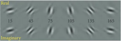
An alternative construction that achieves both lower overcompleteness (and therefore is more efficient), yet also displays good shift-invariance and higher angular selectiv-ity is the dual-tree complex wavelet transform (DTCWT) pioneered by Kingsbury [111], illustrated inFigure 7. This complex transform has found applications in motion estima-tion, interpolaestima-tion, denoising, and keypoint detection [112]. One problem with the original DTCWT transform is that de-spite its higher angular selectivity, the highpass channels do not lend themselves to easy orientation steering (i.e., altering only the angular tuning of the filtered response using out-puts of filters at only a single scale). A recent modification of the tree [113] yields near rotation invariance, and con-sequently orientation steerability within any one scale (see
Figure 8). This makes the patterns of coefficients very stable
Real
Imaginary
15 45 75 105 135 165
Figure7: Impulse responses of original construction of Kingsbury’s complex dual-tree wavelets.
Real
Imaginary
15 45 75 105 135 165
Figure8: Impulse responses of original construction of Kingsbury’s modified complex dutree wavelets. Note that as direction is al-tered, the number of cycles per envelope remains approximately constant, which is directly associated with the property of approxi-mate rotation invariance.
under rotations, yet keeps the redundancy less than that of the fully shiftable, rotationally steerable framework of an undecimated construction, such as Freeman and Adelson’s. Variations on these constructions have been pursued by Se-lesnick [114].
As mentioned earlier, the DTCWT has found applica-tions in image denoising. Perhaps one of the best performing denoising systems is based on the steerable complex pyramid of Portilla et al. [115], where very high angular selectivity is used, by employing as many as 12 orientation channels. Another interesting demonstration of denoising by struc-tural detection using the steerability properties of a steerable wavelet decomposition was suggested by Bharath and Ng [116]. Ng and Bharath have also shown that color opponent wavelet decompositions based on complex steerable wavelets permit the detection of perceptual boundaries [117], that is, both edges and line-line structures, even at single scales.
The parallels to V1 computation in the scale-space par-adigm are formulated in terms of partial derivatives of a multiscale image representation, in which the original im-age lies “embedded” at the finest scale of this representation. First and pure second-order linear Cartesian derivatives are similar to symmetric and antisymmetric receptive fields of V1 neurons, although it is quite common in scale-space ap-proaches to use isotropic Gaussian kernels as the scale-space generator.
A variety of simple cells with the same orientation preference,
but different phases of RF Concept suggested by Hubel and Wiesel, which is to think of the complex cells as arising like this
NL NL NL NL
NL=nonlinearity
Note also that there is evidence of complex cells arising directly from LGN inputs: recurrent models can explain this
Note that this is one class of complex cells, but it is the most commonly used model
Complex response
out
0 5 10 15 20 25 0.15
0.1 0.05 0 0.05
0 20 40 0 5 10 15 20 25 0.15
0.1 0.05 0 0.05 0.1
020 40
0 5 10 15 20 25 0.15
0.1 0.05 0 0.05 0.1
0 20 40
0 5 10 15 20 25
0.1 0.05 0 0.05 0.1
0 20 40
Figure9: Generalized use of nonlinear combination of receptive fields over linear parameter variation to construct invariant feature measure. Note that the number of linear filters depends on parameter characteristics and sharpness of its tuning. For phase-invariant responses from quadrature filters, this reduces to two linear operators/directions.
illustration of this principle. See also [119] for a practical ap-plication in medical blood vessel segmentation.
The primary operators of both the scale-space and filter-bank paradigms are linearand these bear close relevance in-deed to the spatial properties of many V1 receptive fields. However, the majority of V1 receptive fields is actually of a complex nature, by which is meant that usually display spatially phase-invariant properties [120], or other, possi-bly unspecified nonlinearities. Interestingly, there is a generic model for how such properties arise in biological vision, which is efficiently mirrored by signal processing. Thus, in order to “achieve” phase-invariant responses at one angle of orientation, one may use the model shown inFigure 9 (mod-ified from [121]).
Note that for two phases of response that are in ex-act quadrature, the number of linear operators feeding into the nonlinearity in order to generate a phase-invariant re-sponse reduces to two, which are the in-phase and quadra-ture components. Note also, however, that an interesting gen-eralization also emerges: in order to generate a phase- and orientation-invariant measure of the edge likelihood, one may “pool” responses over all phases and orientations, an in-teresting generalization.
It is clear that although there are close analogies to spatial processing operators in image processing and com-puter vision, there remain distinctions in existing spatial processing paradigms: temporal responses in existing image
processing frontends are usuallyδ1(k) functions (withk be-ing frame/time index), whereas there are well-defined veloc-ity tuning characteristics to most V1 neurons. This, we be-lieve, represents a rich source of inspiration for operator de-sign, and presents technical challenges, due to existing band-width shortcomings.
4.2. Theory and model of intracortical
interactions in V1
There have been various attempts to model the intracorti-cal interactions and contextual influences in V1 [122–125]. Since a network with recurrent interactions can easily have all kinds of stability problems, it is difficult to make a well-behaved model that does not generate unrealistic or halluci-native responses to input stimuli, even when the model fo-cuses only on a subset of the contextual influences such as collinear facilitation [123]. Because of this, many models, for example [124,125], do not include explicit geometric or spa-tial relationships between visual stimuli, and thus have lim-ited power to link physiology with visual behavior.
contrast. The model consists of recurrent pairs of excita-tory and inhibiexcita-tory neurons with weighted connections to the output of orientation-selective complex cells and color-opponent centre-surround cells that simulate among oth-ers the effect of isoorientation inhibition, collinear enhance-ment, and color contrast to produce a saliency map; with lo-cally translation-invariant neural tuning properties and in-tracortical interactions, V1 responses highlight the locations where translation invariance or homogeneity in input breaks down on a global scale. These locations can be at texture boundaries, at smooth contours, or at pop- out targets (such as red among greens or vertical among horizontals) in vi-sual search behavior. The recurrent computation of the neu-rons in the model which produces a saliency response is analogous to amaxoperation on different feature saliency maps, whereas other models of saliency such as Itti et al. [127] have usedsumoperators. This theory links V1 physiol-ogy/anatomy with visual behavior such as texture segmen-tation [128], contour integration [129], and pop-out and asymmetries in visual search [130, 131], which have often been thought of as complex global visual behavior dealt with beyond V1. The model proposes that V1 performs the ini-tial stage of the visual segmentation task through the saliency map, and such segmentation has been termed preattentive segmentation in the psychological community. It is termed “segmentation without classification (recognition)” in [33], which relates to the bottom-up segmentation in computer vision. This theory/model has generated testable predictions, some of which have been experimentally confirmed, such as color-orientation interference in texture segmentation [132] and the relationship between border saliency and figure-ground saliency effects [133].
In particular, saliency maps are believed to provide a fast mechanism to direct the focus of attention of the visual pro-cessing system and eye-fixations without having to wait for slower feedback information from the higher-level cognitive areas of the visual cortex. Saliency maps are useful for con-trolling pan-tilt zoom cameras and retinomorphic cameras capable of simultaneous image processing at different reso-lutions.
5. CONCLUSION
Neurophysiological and anatomical experiments have pro-vided new insights into the functions of V1 neurons. The re-sponse of V1 cells has been shown to be more dynamic than previously believed. In particular, the spatial selectivities of V1 cells have been shown to undergo a temporal refinement process of the tuning curve from medium to high frequencies [53]. The underlying mechanism of V1 selectivity has also been shown to be more than a feedforward weighted-sum fil-tering (either linear or non-linear) of stimuli from the recep-tive fields [78]. Lateral connections between V1 neurons and feedback connections from higher cortical areas have been shown to affect the response of V1 cells, and more impor-tantly, determine the role of V1 in high-level visual functions beyond feature detection and representation. The following material could be useful for further readings on the primary
visual cortex. Wandell [12] provides a textbook style intro-duction to physiology and psychophysics of vision in gen-eral. Lennie [9] provides a review of V1 together with a pro-posal for its role in visual feature analysis in the context of functions of extrastriate areas. Martinez and Alonso [120] reviewed the properties and models regarding complex and simple cells. Schluppeck and Engel [134] reviewed and rec-onciled the conflicting evidence about color processing in V1 from optical imaging and single-unit recording data. An-gelucci et al. [135] review the anatomical origins of intracor-tical interactions in V1, while Lund et al. [136] review the anatomical substrate for the functional columns. Reid [137] reviews V1 in a textbook chapter for neuroscience. Fr´egnac [138] reviews the dynamics of functional connectivities in V1 at both molecular and network levels.
We do not cover in this review the topic of development processes of V1, and only briefly cover plasticity and learn-ing. However, the dynamical changes in the properties of V1 neurons and the plasticity of their responses to the immedi-ate history of stimulus presentation, over timescales of mil-liseconds, in addition to the fact that the majority of retinal signals enter the visual cortex through V1, indicate that V1 may play a large role in the plasticity and adaptability of the overall perceptual process of seeing. Chapman and Stryker [139] review the development of orientation selectivity in V1, while Sengpiel and Kind [140] review the role of neural activities in development. The material in this review on the intra-cortical interactions and contextual influences are rel-atively recent, thus further developments and revised points of views on these aspects are expected. Furthermore, there is much interest regarding the possible role of V1 in higher-level cognitive phenomena. These phenomena include alter-native or unstable perceptions (e.g., binocular rivalry when subjects perceive one image of the two different and inconsis-tent images presented to the two eyes), atinconsis-tentional blindness, visual awareness, or consciousness [141,142].
REFERENCES
[1] G. Holmes, “Disturbances of vision by cerebral lesions,” British Journal of Ophtalmology, vol. 2, pp. 353–384, 1918. [2] P. E. Flechsig,Gehirn und Steele, Veit, Leipzig, Germany, 1896. [3] A. Cowey, “Projection of the retina on to striate and prestriate cortex in the squirrel monkey, Saimiri sciureus,”Journal of Neurophysiology, vol. 27, no. 3, pp. 366–393, 1964.
[4] D. H. Hubel and T. N. Wiesel, “Early exploration of the visual cortex,”Neuron, vol. 20, no. 3, pp. 401–412, 1998.
[5] S. A. J. Winder, “A brief survey of central mechanisms in pri-mate visual perception,” preprint, 2002.
[6] B. A. Olshausen and D. J. Field, “How close are we to under-standing V1?”Neural Computation, vol. 17, no. 8, pp. 1665– 1699, 2005.
[7] T. Bolton, “General anatomy of the visual system,” 2002,
http://www.undergrad.ahs.uwaterloo.ca/tbolton/Anatomy. htm.
[8] S. Zeki,A Vision of the Brain, Blackwell Scientific, London, UK, 1993.
[10] L. G. Ungerleider and M. Mishkin, “Two cortical visual sys-tems,” inAnalysis of Visual Behavior, pp. 549–586, MIT press, Cambridge, Mass, USA, 1982.
[11] W. H. Merigan and J. H. R. Maunsell, “How parallel are the primate visual pathways?” Annual Review of Neuroscience, vol. 16, pp. 369–402, 1993.
[12] B. A. Wandell,Foundations of Vision, Sinauer Associates, Sun-derland, Mass, USA, 1995.
[13] B. A. Olshausen, “Principles of image representation in visual cortex,” inThe Visual Neurosciences, L. M. Chalupa and J. S. Werner, Eds., pp. 1603–1615, MIT Press, Cambridge, Mass, USA, 2003.
[14] G. H. Henry, “Afferent inputs, receptive field properties and morphological cell types in different laminae of the striate cortex,” inThe Neural Basis of Visual Function, vol. 4 ofVision and Visual Dysfunction, pp. 223–245, CRC Press, Boca Raton, Fla, USA, 1989.
[15] P. Lennie and J. A. Movshon, “Coding of color and form in the geniculostriate visual pathway (invited review),”Journal of the Optical Society of America A: Optics, Image Science, and Vision, vol. 22, no. 10, pp. 2013–2033, 2005.
[16] E. M. Callaway, “Structure and function of parallel path-ways in the primate early visual system,”Journal of Physiology, vol. 566, no. 1, pp. 13–19, 2005.
[17] H. B. Barlow, “Possible principles underlying the transforma-tion of sensory messages,” inSensory Communication, W. A. Rosenblith, Ed., pp. 217–234, MIT Press, Cambridge, Mass, USA, 1961.
[18] J. J. Atick, “Could information theory provide an ecologi-cal theory of sensory processing?”Network: Computation in Neural Systems, vol. 3, no. 2, pp. 213–251, 1992.
[19] J. J. Atick, Z. Li, and A. N. Redlich, “Understanding reti-nal color coding from first principles,”Neural Computation, vol. 4, no. 4, pp. 559–572, 1992.
[20] F. Allard, “KIN 356 Course Notes Winter 2002,” 2002. [21] E. Kaplan and E. Benardete, “The dynamics of primate retinal
ganglion cells,”Progress in Brain Research, vol. 134, pp. 17–34, 2001.
[22] Z. Li., “Different retinal ganglion cells have different func-tional goals,”International Journal of Neural Systems, vol. 3, no. 3, pp. 237–248, 1992.
[23] A. Eris¸ir, S. C. Van Horn, and S. M. Sherman, “Relative num-bers of cortical and brainstem inputs to the LGN,” Proceed-ings of the National Academy of Sciences of the United States of America, vol. 94, no. 4, pp. 1517–1520, 1997.
[24] G. H. Henry, A. Michalski, B. M. Wimborne, and R. J. Mc-Cart, “The nature and origin of orientation specificity in neu-rons of the visual pathways,”Progress in Neurobiology, vol. 43, no. 4-5, pp. 381–437, 1994.
[25] A. M. Sillito, J. Cudeiro, and P. C. Murphy, “Orientation sensitive elements in the corticofugal influence on centre-surround interactions in the dorsal lateral geniculate nu-cleus,”Experimental Brain Research, vol. 93, no. 1, pp. 6–16, 1993.
[26] A. Das, “Cortical maps: where theory meets experiments,” Neuron, vol. 47, no. 2, pp. 168–171, 2005.
[27] Z. Li., “A saliency map in primary visual cortex,”Trends in Cognitive Sciences, vol. 6, no. 1, pp. 9–16, 2002.
[28] D. H. Hubel and T. N. Wiesel, “Receptive fields, binocular interaction, and functional architecture in the cat’s visual cortex,”Journal of Physiology, vol. 160, no. 1, pp. 106–154, 1962.
[29] M. C. Morrone and D. C. Burr, “Feature detection in human vision: a phase-dependent energy model,”Proceedings of the Royal Society of London. Series B. Biological Sciences, vol. 235, no. 1280, pp. 221–245, 1988.
[30] M. J. Tov´ee,An Introduction to the Human Visual System, Cambridge University Press, Cambridge, UK, 1996. [31] V. Dragoi and M. Sur, “Dynamic properties of recurrent
inhi-bition in primary visual cortex: contrast and orientation de-pendence of contextual effects,”Journal of Neurophysiology, vol. 83, no. 2, pp. 1019–1030, 2000.
[32] Z. Li., “Contextual influences in V1 as a basis for pop out and asymmetry in visual search,”Proceedings of the National Academy of Sciences of the United States of America, vol. 96, no. 18, pp. 10530–10535, 1999.
[33] Z. Li., “Visual segmentation by contextual influences via in-tracortical interactions in primary visual cortex,” Network: Computation in Neural Systems, vol. 10, no. 2, pp. 187–212, 1999.
[34] Z. Li., “Pre-attentive segmentation in the primary visual cor-tex,”Spatial Vision, vol. 13, no. 1, pp. 25–50, 2000.
[35] D. H. Hubel and T. N. Wiesel, “Ferrier lecture. Functional architecture of macaque monkey visual cortex,”Proceedings of the Royal Society of London. Series B: Biological Sciences, vol. 198, no. 1130, pp. 1–59, 1977.
[36] M. S. Livingstone and D. H. Hubel, “Anatomy and physiol-ogy of a color system in the primate visual cortex,”Journal of Neuroscience, vol. 4, no. 1, pp. 309–356, 1984.
[37] G. Blasdel and D. Campbell, “Functional retinotopy of mon-key visual cortex,”Journal of Neuroscience, vol. 21, no. 20, pp. 8286–8301, 2001.
[38] C. E. Landisman and D. Y. Ts’o, “Color processing in ma-caque striate cortex: relationships to ocular dominance, cy-tochrome oxidase, and orientation,”Journal of Neurophysiol-ogy, vol. 87, no. 6, pp. 3126–3137, 2002.
[39] R. L. De Valois, D. G. Albrecht, and L. G. Thorell, “Spatial frequency selectivity of cells in macaque visual cortex,”Vision Research, vol. 22, no. 5, pp. 545–559, 1982.
[40] M. S. Gazzaniga, R. Ivry, and G. R. Mangun,Fundamentals of Cognitive Neuroscience, W. W. Norton, New York, NY, USA, 1998.
[41] R. D. Freeman, “Cortical columns: a multi-parameter exam-ination,”Cerebral Cortex, vol. 13, no. 1, pp. 70–72, 2003. [42] K. A. C. Martin, “From enzymes to visual perception: a
bridge too far?”Trends in Neurosciences, vol. 11, no. 9, pp. 380–387, 1988.
[43] D. J. Felleman and D. C. Van Essen, “Distributed hierarchical processing in the primate cerebral cortex,” Cerebral Cortex, vol. 1, no. 1, pp. 1–47, 1991.
[44] G. C. DeAngelis, G. M. Ghose, I. Ohzawa, and R. D. Freeman, “Functional micro-organization of primary visual cortex: re-ceptive field analysis of nearby neurons,”Journal of Neuro-science, vol. 19, no. 10, pp. 4046–4064, 1999.
[45] L. M. Martinez and J.-M. Alonso, “Construction of complex receptive fields in cat primary visual cortex,”Neuron, vol. 32, no. 3, pp. 515–525, 2001.
[46] D. L. Ringach, M. J. Hawken, and R. Shapley, “Temporal dy-namics and laminar organisation of orientation tuning in monkey primary visual cortex,” inProceedings of European Conference on Visual Perception (ECVP ’98), Oxford, UK, Au-gust 1998.
![Figure 2: Illustration of a hypercolumn containing neurons selec-tive to orientation, ocular dominance, and color, obtained from[40].](https://thumb-us.123doks.com/thumbv2/123dok_us/1144837.1143633/5.600.71.271.291.423/figure-illustration-hypercolumn-containing-neurons-orientation-dominance-obtained.webp)