The Diffractive Dissociation Process at π^-p → π^- (π^-π^+p) 14 GeV/c

THE DIFFRACTIVE DISSOCIATION PROCESS TI- p ~TI- (TI-TI+p) AT 14 GeV/c

Thesis by Leo C. Rosenfeld

In Partial Fulfillment of the Requirements for the Degree of

Doctor of Philosophy

California Institute of Technology Pasadena, California

1977

ii

ACKNOWLEDGEMENTS

The experiment which I describe in this thesis depended on the efforts of many people at three institutions. The support personnel of the Caltech High Energy Physics Group built substantial portions of the apparatus. At the Stanford Linear Accelerator Center the major con-tributors were the members of the Experimental Facilities Department, under the leadership of E. Seppi, especially J. Murray; the members of the Accelerator Operations staff; and the members of the Bubble Chamber Operations Group, under the leadership of R. Watt, especially G. Bowden. The scanning and measurement of the bubble chamber film at Lawrence Berkeley Laboratory was in the hands both of the Data Handling Group under the leadership of H. White and the scanning and measuring staff of the Ely Physics Group.

The physicists who played major roles in the work reported here were R. Ely, D. Grether, and P. Oddone of LBL and W. Ford, V. Davidson, F. Nagy, and C. Peck of Caltech. Professor Ely was my host during a long residence in Berkeley, and he generously made available all the resources necessary to carry out the analysis. Professor Peck, the guiding hand and chief stimulus to the entire enterprise, was my thesis adviser. His labor, his leadership, and his friendly counsel were integral to the execution of this. project.

; ; ; ABSTRACT

We describe an experiment in which a 14 GeV/c TI- beam was inci-dent on a hydrogen bubble chamber. Fast forward scattered pions traversed a wire spark chamber spectrometer downstream of the bubble chamber.

Events identified as inelastic by the spectrometer induced a trigger of the bubble chamber camera. The film produced contained a heavy enrich-ment of events of proton diffractive dissociation.

We have studied a sample from this exposure of 4400 events of

- - - - +

the reaction TI p ~ TI N* ~ TI TI TI p. In the two body mass spectra the only noteworthy feature is the 6++(1230). In the N* mass spectrum we observe enhancements at 1.49 GeV, 1.72 GeV, and 2.0 GeV. For the prom-inent 1.72 GeV feature we give estimates of the width and cross section as well as evidence favoring a substantial branching fraction to

TI6(1230). We looked for production of N*(l470) followed by decay to TI6(1230) with negative result. An examination of the 6++(1230) decay distribution suggests that the Deck mechanism is the major contributor to the TI6 subchannel.

iv CONTENTS

Page

ACKNOWLEDGEMENTS . . . • . . . • . . . ii

ABSTRACT CHAPTER

...

,

... .

iii

I. INTRODUCTION 1. The Diffraction Picture of Good and Walker ... 1

2. Properties of Diffractive Dissociation ... 6

3. The t-channe1 Viewpoint • . . . • . . . . • . . . 10

4. The Deck Mechanism ... ,... 13

5. Some Published Data at Very High Energy ..•... 16

6. Intent of the Present Experiment... 21

II. EXPERIMENTAL APPARATUS 1 . Ov e rv i ew ••.•....••.•.•••.••••••• , . . • • • • • • • • • . • • . 2 4 2. The Secondary Beam Line . . . • . . . . • . • . . . • . . . 25

3. The Bubble Chamber ...••..••.•.... 27

4. The Spectrometer... 29

5. Triggering and the Role of the Online Computer .. 34

III. PROCESSING l . Overview ... ~ . 43

2. Processing of the Spark Chamber Data .•...•... 43

3. Scanning and Filtering •..•...•.•.•...•.•.••. 46

4. Measuring ...•...•..•.•..••.. 47

5. Geometrical Reconstruction ...•..•.. ,... 48

6. Hybri di zati on ...•.. , 49

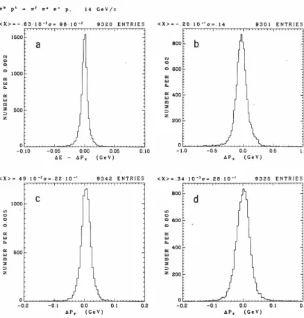
7. Kinematic Fitting •...•.•••.••..•••••..••••.•. 58

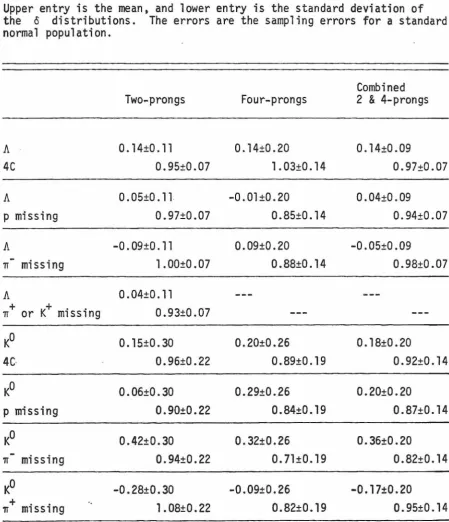
8. Validation... 61

IV. ANALYSES l . Preamb l e ...•...• , .••.••.•... , . . • • • • • • • • 6 9 2. Estimation and Display of Densities .•...•••••.•• 70

3. Event Selection .•..••.•...•.•...•.••..•••••••• 71

4. Normalization ... .... ...•...•.. 80

5. Acceptance and Weighting ..•.•...•••..•..•..••• ,. 82

6. Survey of the N* Mass Spectra .•.••.•••••..•.•... 85

v

Page 8. Further Discussion of N* Resonance Production.... 111 9. Helicity Conservation . ... ... ... •...•••••. •.. 116 10. Test of the Bia~as-Dabkowski-Van Hove Hypothesis . 128

11. SuIT111ary ••••••••••••••••••••••••••••••••••••••••• 141

APPENDICES

A. Deta i 1 s of the Trigger Program . . • . . • . . • . . • . . . • . • • . • • 142 B. The Kuiper Statistic ...•...•...•..• 145 C. The

x

2 Dependence of Contamination

from Lower Constraint Cl asses .•..•.•...•...•...• , . . 149 D. Estimation of the Probability of Track Inversion ... 151

1

I. INTRODUCTION

1. The Diffraction Picture of Good and Walker

In hadron scattering at high energy the preeminent diffractive

process is forward elastic scattering. We call it diffractive because

the dominant features of this process are understandable from the

view-point of optical diffraction. The target acts as a nearly opaque disk,

extinguishing most of the incident wave. The resulting shadow acts, in

the Huygens construction, as the source of secondary waves at small

angles from the incident direction. We refer to certain inelastic hadron

processes as diffractive dissociation. They are similar in their major

properties to elastic scattering, and they may also be a result of

absorption of the incident wave.

The first thorough exposition of the concept of diffractive

dissociation appears in Good and Walker [1960]. They present the following

optical analogue. In the case that a linearly polarized wave impinges

on an opaque disk, the diffracted light has the same polarization as the

incident light. Suppose instead that the disk is a Polaroid and that its

axis is at 45° to the direction of polarization of the incident wave.

The polarization of the diffracted wave is then transverse to the axis of

the Polaroid. If we project the diffracted wave on axes parallel and

perpendicular to the incident polarization, we find components in both

directions. Diffraction by a Polaroid can thus create a new state, one

not present in the incident wave.

2 1.1

AB + A* B (1.1)

in which B is a nucleus, A is a meson or nucleon, and A* is a system of two or more hadrons which are the dissociation products of A. They adopted the viewpoint that a hadron is a composite of more elementary objects. One representation of a free particle state is a superposition of states containing different numbers and kinds of constituents.t

The choice of basis is at our disposal. For representing the incident hadron, A, and the final hadrons, A*, the appropriate basis is the set of states

10.

₁

>

of one or more free particles. For understanding the propagation of the constituents of A through B, the appropriate basis is the set of states IC;> which the nuclear matter attenuates

exponentially. In general the rate of attenuation would be different for each IC;> , and in general no IC;> would be a free particle state.

We represent the incident hadron A as

101

>

=

~

c. IC;> 1 1

(1. 2)

The transmitted wave is

IT>

=

I

n· c. IC;> 1 1 1

( 1 • 3)

3 I. l

with

In .1

_l < 1 We reproject

IT>

into the

ID; >

basis obtaining

I

13;

10.>

i > 1 1 1

( 1 . 4)

f3; = <D;

IT>

=

I

n .c. <D.

I

c.

>

j J J 1 J ( 1. 5)

The first term on the right of equation (1.4) interferes with the incident

wave to produce elastic scattering. The second term on the right is a

source of secondary waves of one or more free particles distinct from the

incident hadron. It corresponds to the new polarization state which we

found in considering diffraction from a Polaroid.

An elegant example of differential absorption in hadronic

reac-tions is the regeneration of Ks from KL in nuclear targets. The

incident KL is a superposition of equal parts of the strangeness

eigen-states KO and

K° .

The nuclei of an absorber attenuate these states

at different rates, so the emergent state is a superposition of KL and

Ks .

In the foregoing analysis we ignored the phase change of the

hadron wave function as it propagates through a nucleus. This

4 I. l

extent in the beam direction or if all the states jc. > and

,

jD. > were

,

energy degenerate. In the general case, however, many of the states

ID;> have appreciably greater mass than the incident hadron. In

particular the mass of the final state of a dissociated nucleon is greater

by at least the pion mass. We can follow the argument of Good and Walker

to understand how nearly degenerate the jc.> and

,

ID;> states must

be when we treat the nucleus as a three dimensional object. We view

each differential layer of the nucleus as an independent source for the

transmitted wave. At the time of excitation, a layer emits a

superposi-tion of the states ID;> in phase with the incident wave. Each ID.>

,

then propagates with a frequency dependent on its mass to the shadow side

of the nucleus. For masses too far from that of the incident hadron the

layers contribute incoherently to the final state and a significant cross

section can not develop. Diffractive dissociation, in the sense of Good

and Walker, is the relatively large cross section expected when the

initial and final states are so nearly degenerate that the wavelets from

each layer of the nucleus are in phase when they emerge.

We make the above considerations quantitative as follows. The

frequency difference of the A and the A* systems of reaction (1.1)

is proportional to their energy difference.

~w

=

(E* - E)/h (1.6)

5 I. 1

( 1 . 7)

rA and r 6 are the radii of A and B, and the factors 1/y account for the Lorentz contraction. The coherence condition is

1::,w flt << 1 . (1.8)

We evaluate E*-E from energy-momentum conservation, and we approximate both rA and r₈ by the Compton wavelength of the pion, hc/mn. The general result is

+

J

<< l . ( l . 9)

s is the square of the center-of-mass energy, and M* is the mass of

A* • We specialize relation (1.9) for three cases which cover most

situations of practical interest.

Case l. MA<< M_{8 , B} is the target, A has momentum P >>MA

Case 2.

m

7T

6

2MA

• - << 1

s

or with P the beam momentum in the rest frame of either A or B

m p

7T

<< 1 .

I. l

(1. 11)

(1.12)

Case 3. M8 << MA ,

M~

<< s , P is the momentum of B in the A rest frame.

2m P

7T

<< 1 (1.13)

Relations (1.10)-(1.13) make clear that the higher the beam momentum,

the higher the M* at which diffractive dissociation may be observable.

2. Properties of Diffractive Dissociation

The connection between quantum number exchange and energy

depen-dence is the feature of hadronic processes which pennits us to distinguish

phenomenologically between diffractive dissociation and other dissociation

processes. Over the domain of presently available energies two-body

7

o{AB ~ A*B) ~ p -r

When A* has the same internal quantum numbers as A,

r S 0.5

whereas when A* has different internal quantum numbers, r ~ 1.5

[Fox and Quigg 1973].

I.2

{2.1)

{2.2)

All proposed models of diffractive dissociation are unanimous in

support of a selection rule requiring A* to have the same quantum

numbers as A. In the absorption model of the preceding section this

rule is an irrrnediate consequence for the additive quantum numbers.t

In the case that A is a meson with definite charge conjugation CA ,

the model does not by itself require that CA*

=

CA . The Pomeranchuk

theorem, however, which asserts the equality of particle and antiparticle

cross sections at infinite energy, disfavors a gentle energy dependence

like {2.2) if CA* ~ CA . Although the model of Good and Walker is

relevant to Ks regeneration as we mentioned, the charge conjugation

changes from KL to Ks' and the process does not satisfy relation

(2.2). [Brody et al. 1971]. A corollary of the preservation of the C

quantum number is that pions dissociate only into odd numbers of pions

because the dissociation products must preserve the G parity.

Corresponding rules for K meson diffractive dissociation are obtainable

by invoking SU{3) syrrmetry.

8 I.2

Diffraction scattering characteristically produces an angular

distribution with a sharp forward peak. The Heisenberg uncertainty

principle relates the width of the peak to the size of the diffracting

object.

P ~ h/r

t (2.3)

with Pt the momentum component transverse to the incident direction

and r the radius of a black disk. Elastic scattering of hadrons from

nuclei exemplifies this behavior [Blieden et al. 1975 and Apokin et al.

1976]. Good and Walker [1960] reason that since absorption is

respon-sible for both elastic diffraction and diffractive dissociation, the

production angular distributions should be similar. Differences might

exist, however, because the transparency of the absorbing disk may depend

on impact parameter. Some other models in the same spirit as Good and

Walker yield more detailed predictions for the angular distribution in

dissociation reactions [Chou and Yang 1968, Cheng and Wu 1971].

A selection rule for the internal angular momentum and parity

of A* is a more difficult matter than the selection rule for the

internal quantum numbers, in part because the quantum number accounting

must include the orbital angular momentum of A and A* with respect

to B. Good and Walker suggested that the orbital angular momentum would

not change with.the consequence that JP(A*)

=

Jp(A). In discussions

of Regge exchanges Gribov [1967] and Morrison [1968] proposed the less

9 I.2

P(A*)/P(A) = (2.4)

as a property of Pomeron exchange (see the following section).t Both authors spoke of A* as a resonance, and neither specifically addressed the question of whether the rule should apply to a nonresonant component of A* . Carlitz et al. [1969] proposed yet another rule stating that a resonant A* could belong only to certain SU(6) multiplets. Experi-ments have not clearly established the validity of any of these rules.

A different kind of angular momentum rule concerns the helicity of A*. For zero degree scattering (and assuming no B spin flip) the helicity of A* must be the same as the helicity of A purely to conserve angular momentum. When the scattering angle is nonzero,

statements about the A* helicity must refer to a particular reference frame. Experimental evidence favors helicity "conservation" in the center-of-mass frame for TIP elastic scattering (A = p, A* = p) and for the quasi-elastic process yp +pop (A = y, A*= PO) (references in Section IV.9). This rule does not appear to be valid for meson and baryon dissociation reactions, at least not generally. An alternative rule, helicity conservation in the A* rest frame (t-channel helicity conservation), has some experimental support. As with the Gribov-Morrison

10 _I.2

rule the helicity conservation properties of A* may depend on whether or not A* is resonant.

3. The t-channel Viewpoint

Our present understanding of nondiffractive two-body processes at lab momentum ·~ 4 GeV is in tenns of particle exchange in the t-channel. The 11

t-channel11 _{of the reaction AB+ C 0 is the reaction}

AC

+

B

0 . We describe both reactions with a single amplitude

analytically continued in the variables

2

t

,J

(Pc - PA)2 s-channel

(PA + PB)

s

-2

·

I

(Pc+ PA)2 t-channel

(PA - P _) B

(3 .1)

11 I.3

and a forward peak in dcr/dt is generally not evident.

The extension of these ideas to account for the combined effect

of all possible t-channel exchanges is the Regge pole phenomenology. In

the Regge analysis the amplitude for the s-channel reaction has the

following integral representation when A, B, C, and D are all spinless

(the Sommerfeld-Watson transfonnation).

M{s,t) = 1 2Tii

f

(2L+l) PL (-z(s,t))

sin TI L A(L,t)dL

c

(3.2)

The function z(s,t) is the cosine of the scattering angle of the

t-channel reaction. Kinematics alone detennines its fonn. The function

PL is the Legendre function of complex order L and degree zero. The

functions obtained by restricting A(L,t) to non-negative integer values

of L are the partial wave amplitudes of the t-channel reaction. The

contour C encloses at least these values of L . In the theory of

scattering from a potential the singularities of the function A(L,t) in

the complex L plane are isolated poles. They are the Regge poles, and

their positions, ai(t), are the Regge trajectories. The rightmost pole,

the one with the largest Re a , dominates the behavior of M(s,t) in

the large s limit.

For relativistic particle scattering the singularities of A(L,t)

may in principle be more complicated than isolated poles. The simple Regge

12 I.3

description of much of two-body scattering data [Fox and Quigg 1973) but also connects it with particle spectroscopy. A value of ,If (t > 0) at which a(t) is a non-negative integer (of proper signature) is the

expected mass of a particle or -resonance, and the usual identificaticm of a trajectory is by the name of the lowest mass state which lies on it, for example the "p trajectory." A special trajectory, however, is the

"Pomeron.11

All of its t-channel quantum numbers are zero, and therefore the lowest mass state on it is the vacuum. From the t-channel viewpoint the Pomeron is the basis for understanding elastic scattering and

inelastic diffractive processes. The Pomeron pole is always to the right of the other Regge poles, so when its exchange is possible, it dominates in the high s regime.

The two chief results of the Regge theory are the s dependence of dcr/dt and factorization. When only Pomeron exchange need be

considered,

do 2a (t)-2

= R(t) s J:

dt (3.3)

with ~(t) the trajectory of the Pomeron. This same s dependence obtains regardless of the identities of the initial and final state particles. The content of factorization is that R(t) is a product of two factors, one depending only on the t-channel initial state, the other depending only·on the t-channel final state.

13 I.3

Experimentally testable corollaries take the fonn

da dt AB + A*B

da/dt AB + AB

=

da/dt AC + A*C

da/dt AC + AC (3.5)

Beyond factorization Regge theory leaves considerable freedom in the fonn of the functions R(t).

For the understanding of reactions in which the quantum numbers forbid Pomeron exchange, the Regge phenomenology has no peer. The Pomeron, however, has been an object of substantial controversy. If the absorp-tion mechanism described in Secabsorp-tion I.l is a correct view of diffractive reactions, then it is not clear why the Pomeron singularity should have the simplicity of a Regge pole. The predictive powers of the two view-points do not have much overlap, so experiment does not easily discrimi-nate between them. A recent review of hadron diffraction theory empha-sizing the t-channel viewpoint is available in Abarbanel [1976].

4. The Deck Mechanism

Drell and Hiida [1961] and Deck [1964] proposed the following mechanism as a contributor, at least, to diffractive dissociation. One of the incident particles dissociates virtually into two pieces, for

example TI + pTI or p + TIP • One of the pieces then scatters elastically

14 I.4

B

---

B'

D propagator •---DB elastic scattering

r - - - o

A

c

FIG. 1. Diagram representing the Deck mechanism.

Since the fraction of A's time which it spends as a virtual state of C

and D is independent of beam energy, the energy dependence of the

process is like the energy dependence of DB elastic scattering and is

therefore diffractive.

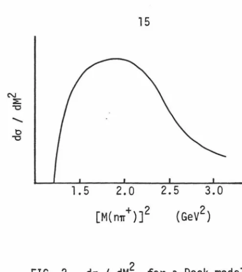
A characteristic of the Deck mechanism is that it produces a

broad enhancement near threshold in do/dM(CD) without the need for

resonance fonnation in the CD system. We illustrate this in Figure 2

using do/dM2 for a particular Deck model fitted to data of the reaction

+

15

2.5 3.0

(GeV2)

FIG. 2. do/ dM2 for a Deck model.

I.4

Experimentally the do/dM for the diffractive dissociation of any

incident hadron, n , K, or nucleon, exhibits a threshold enhancement

(A

1, Q, or U*). Deck models tend, however, to overestimate its width.

The Deck mechanism also predicts the distribution in the variable

t(BB') [Oh and Walker 1969]. In a fit of the cross section to the form

exp[-b(M)t(BB')]

the expected result is a b(M) which decreases dramatically with

increasing M in the regime just above threshold.

From the t-channel viewpoint (preceding section) the Deck

mechanism is just a special case in which the Pomeron exchange mediates

the BD elastic scattering. By adding details of the dynamics at the

16 1.4

is not an intrinsic part of Pomeron phenomenology,

5. Some Published Data at Very High Energy

We do not undertake in this sec ti on a general review of the ·

experimental work on diffractive dissociation. Several such reviews are

available [Derrick 1975, Miettinen 1975, Leith 1974, Gramenitskii and

Novak 1974, and works they reference]. We merely want to point to four

recent published experiments which demonstrate dissociation of the

nucleon into exclusive channels at 20 GeV/c to 1000 GeV/c equivalent

beam momentum. All four experiments used electronic detection methods.

The first group [O'Brien et al. 1974] studied the reactions

n C -+ p 1r C

n Cu -+ p 1r Cu .

( 5. l}

(5.2)

The spectrum of their neutron beam peaked at 25 GeV/c and was 8 GeV/c

wide (FWHM). We reproduce some of their results in Figure 3. The

most noteworthy feature of this data is that none of the well established

N* resonances appear as obvious peaks.

The second experiment [Edelstein et al. 1977] obtained data for

the reactions

+

-pZ+p7r 'IT Z (5.3)

500

~

400

..

..,

..

0 0

300

~ .._

..

..

c:

..

>

200

w

JOO

l

°tos

-

---...

1470

i

...

...

1.2

L4

...

Carbon 0. 0<11'1

<O. 04 IGeVlcl 2 P1pn-1 > 20 Ge Vic

168S

l

Accept once ... ... ...

___

_

l6 LS C•V M(p1r-) for carbon

• u c:

50

~ a.

..

u u ~

25 Coherl'nt production cross section versus !ti (pir-)

240 2(11)

>

160

., Cl 0 ~

120

"' c ., ,. w

80 40 0

LZ l4 M(pir-) for copper Target 1.078 <M(pir-)< l.S GcV 1.4 < M(p,,-)< 1.6 GeV 1.5<M(p,,-)<1.8 GeV

c Cu

1.00 t 0.27 mb 0.37 t 0.13 mb 0.23 t 0.07 mb 2.27 t 0.47 mb 0.73 t 0.19 mb 0.36 t 0.16 mb FIG. 3. Figures and table from O'Brien et al. [1974].

Copper 0. 00

< lt'I < 0. 02 IGeV/cJ2 Ptpn-I > 20 GeVlt GtV

15 001~

r

·oo

1200

1

9 00]

I

:. 6 00

~

~

~ 50

l

3 0 0 ~,__ ~ ~~~~ ~~ ~~~~~o 1 . 35 I 5 0 1 . 65 I 8 0 I 95 2 10 Mau ( p,.,• .• -)f G tV) Unc o rrected p1T+1T· mass spectrum for p +C -p1T+1T· +Cat 22.5 GeV with -t' < 0.04 (Gev/cl 2• Geo-metrical acceptance o f the spectrometer vs mass ls su-perimposed. FIG. 4. Figure from Edelstein et al. [1977]. ~ 35 0 '-' 2J

11

0 . 1, -14 0 . 6 Go v '

N 0 0

6

7

3

1

'"'"''

' ~ c

210

..

>

..

·::

1

~

I:

~

0 ~

..

u

E

c

,

0

z

~ u u

..

1 .2 1 .4 1 .6 1. 8 2-0 2-2 2" 2 . 6 . 28 3 . 0 M ( p .... " -l (GtV I + -Experimental distribution in #(pw w ) for 0.1 S -t ~ 0.6 GeV 2 • The smooth curve is the acceptance.

_, 00

FIG. 5. Figure fro m Webb et al. [1976].

1200

I

(a>

900 6001

(

4\__

300 -~ -1.-2 1.4 1.6 1.8 900 I (b) _,,

.rf[

5

~

600 I 300 I 1.2 1.4 1.6 1.8 900

I

(c)

/ii\~

600! 300

I

r

1.2 1.4 1.6 1.8 (GeVl MASS p-rr-Mass spectra of prr-pairs In hydrogen, Inte-grated over a 50-300 GeV le neutron momentum band, displayed as a function oft . (a), (b), and (c) corre-spond to It I bands of 0.02-0.08, 0.08-0 . 20, and 0.20-1.00 Ge V 2, respectively.

a

:0 ::1..

60

~ z 0 ~

40

u w (/) (/)

20

(/) 0 a: u

o

1.35<M<l.45

•

1.25<M<

1.35

-+-r+~

·+~

100 200 300 NEUTRON MOMENTUM (GeV/c) Energy dependence of the cross section for two low-mass intervals. Data are shown Integrated over O .02 <It I< 1.0 Ge V 2 • The absolute normalization Is uncertain by about :i 20%

.

b

FIG . 6. Figures from Biel et al. [1976].

20 I.5

momentum was 22.5 GeV/c. In Figure 4 we show their p TI + -TI mass spectrum for the carbon data. Peaks are evident at about 1.4 GeV and

1.68 GeV. Whereas the lower peak could as well be a kinematic enhancement

(see the preceding section), the upper peak is more suggestive of a

resonance.

The reaction

n p ~ p TI p (5.4)

was the subject of the third experiment [Biel et al. 1976]. The neutrons

delivered by a neutral beam at Fennilab had momenta in the range 50-300

GeV/c. In Figure 6 we reproduce the pn- mass spectrum and the cross section as a function of neutron momentum. The mass spectrum suggests

some resonance production in the vicinity of 1.65 GeV. Figure 6b

shows that the energy dependence of the cross section is indeed as

expected for a diffractive process.

Our final example is an experiment conducted at the CERN-ISR

[Webb et al. 1975] to study the reaction

(5.5)

The momenta of the colliding beams were both 22 GeV/c which is equivalent

to a beam momentum of 1000 GeV/c for a fixed target experiment. The

mass spectrum obtained appears in Figure 5 • This spectrum suggests

21 I.5

experiment on nuclei (see Figure 4 ). The relative dearth of events

at the low mass end is most likely an artifact of the t selection, The

Fermilab data (Figure 6 ) shows how sensitive the mass spectrum can be

to the t cut. Much of the reaction (5.5) cross section corresponds to

!ti < 0.1 which is the lower limit of the ISR data. To estimate this

cross section including the unobserved small !ti region, Webb et al.

extrapolated their observed t distributions to t

=

0. Their result

is 0.33 ± 0.1 mb at Plab

=

1000 GeV/c and 0.34 ± 0.1 mb at

Plab

=

1500 GeV/c. The absence of strong energy dependence characterizes

the process as diffractive.

Taken together these four experiments show that, at high energy,

nucleons dissociate into exclusive channels with cross sections of the

order of 200 µb and that the cross sections are roughly independent of

energy. Three of them suggest that a small part of the cross section

is attributable to resonance production.

6. Intent of the Present Experiment

Prior to the proposal of this experiment, missing mass

measure-ments [Belletini et al. 1965, Anderson et al. 1966, Foley et al. 1967]

had provided large sample mass distributions and differential cross

sections for nucleon diffractive dissociation. Peaks in the mass spectra

suggested resonance production but could reveal nothing about their decay.

More information was necessary to confront several questions. l) How

much of diffractive dissociation was ascribable to resonance production

22 I.6

produce? 3) Did their production angular distributions have forward

dips? 4) What was the status of the Gribov-Morrison and the helicity

conservation rules? Attacks on these questions required studies of the

angular distributions and correlations of the dissociation products.

For this kind of work the superior 4TI detection efficiency of a

bubble chamber is a considerable advantage, but the individual exposures

then available were not large enough. The objective of the present

experiment was a manyfold increase in the number of photographs of

proton diffractive dissociation.

We pursued this objective by means of a synergistic combination

of spark chamber and bubble chamber techniques. In the traditional mode

of operation bubble chambers produced a picture of every beam pulse

regardless of what sort of events occurred. This mode was not an

economical way to obtain a large sample of a particular channel which

was but a small fraction of the total cross section. The dissociation

channels p + p TI 0 , p + n TI + , and p + p TI + -TI represent about 5%

of a total cross section of 26 mb for TI- p interactions at 14 GeV.

We partially remedied the slectivity problem of the bubble chamber by

augmenting it downstream with a wire spark chamber spectrometer. The

spectrometer discriminated proton diffractive dissociation events both

from elastic scatters and, by its limited acceptance, from much of the

rest of the inelastic cross section. The bubble chamber camera produced

a picture only on pulses for which the spectrometer indicated the

23 I.6 By these means we collected film containing about 45 events/µb for the part of the cross section that we wished to investigate. What we achieved was about one half of our original goal, Chapters II and III document our methods, and in Chapter IV we present some analyses of the

- - +

TI TI TI p final state.

Before ·proceeding we issue one caveat. From the point of view of the absorption mechanism (Section I.l) our beam momentum is uncomfortably low. The inequality (l ,13) has the form f(M*)/P << 1. Below

we graph f(M*) and compare it with 14 GeV/c, the highest beam momentum available to the experiment. That the graphs cross at a comparatively low value of M* is certainly unfavorable. This situation is not directly relevant to our own analyses because in Chapter IV we do not explicitly treat our final state as a consequence of absorption.

20

-

15 Our beam

>

_cu ..._momentum

<.!)

--

10

*

~

-

-

5

0

1.0 1.5 2.0 25

24

II. EXPERIMENTAL APPARATUS

l. Overview

The major components of the apparatus were the 4011

hydrogen

bubble chamber at the Stanford Linear Accelerator Center (SLAG), a large

aperture magnetic spectrometer installed downstream of the bubble

chamber, a beam line to deliver n- mesons from the primary target, and

a Xerox Sigma 2 computer. Briefly these components functioned together

as follows. Prior to delivery of a beam pulse the bubble chamber began

its expansion, and the cycle followed its normal course regardless of

the scattering of any beam particles. The computer controlled only the

bubble chamber camera. On most pulses the film remained unexposed. If

an appropriate interaction did occur, some scintillation counters

detected the forward scattered particle and triggered the wire spark

chambers of the spectrometer. The spark chamber electronics digitized

the spark positions and transferred this infonnation to the computer.

During the time required for bubbles to develop in the chamber, the

computer analyzed the spark data to ascertain the momentum of the

forward scattered track. If this momentum was within a preselected

range, the computer signaled the bubble chamber camera to expose the

film. Whenever the computer received spark digitizations it recorded

them on magnetic tape.

In the rest of this chapter we describe the apparatus and the

25 II. 2

2. The Secondary Beam Line

The SLAC accelerator delivered an intense beam of 19 GeV

electrons to a 30 cm beryllium wire target. The function of the beam

line was to fonn from the secondary emission of the target a low

intensity 14 GeV TI- beam and transport it to the bubble chamber. In

Figure 7 we show a schematic of the secondary beam line. It

collected particles emerging at 17 mrad from the primary beam direction

and had an aperture of about 50 µsr. The beam line had two points

which were foci in both the horizontal and vertical planes. At the

first focus the beam passed through 1.1 radiation lengths of lead to

degrade the momentum of the electron component. Final momentum

defi-nition occurred at a one meter iron slit at the second focus. The last

leg of the beam line gave the beam a ribbon like confonnation at the

bubble chamber. The quadrupoles made the beam parallel in the vertical

plane and focussed at the bubble chamber in the horizontal plane. The

optical axis of the bubble chamber camera was horizontal, so the camera

viewed the broad dimension of the beam. The dipole magnets in the last

leg steered the beam to the correct position and angle for passage

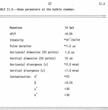
through the bubble chamber and spectrometer. In Table II.A we give

the characteristics of the beam at the bubble chamber. The infonnation

on contamination from K-,

p,

andµ- comes from Boyarski et al.

[1968]. The infonnation on e contamination comes from our own

measurement with a shower counter. The method ultimately used to

l m Fe slit Legend: C, collimator 0, dipole magnet F, focus Q, quadrupole magnet TC, primary target 30 cm Be wire

I20

cm TC31 • ~

~

e beam, 19 GeV FIG. 7. Elevation view of the secondary beam line. The function of this beam line was to form a 14 GeV/c n-beam and transport it to the bubble chamber. All major bends were in the -vertical plane. The field strengths in the horizontal trim magnets 00.5, 02.1, and 03.l were nominally zero.

27

TABLE II.A.--Beam parameters at the bubble chamber.

Momentum

t:.P/P

Intensity

Pulse duration

Horizontal dimension (5% points)

Vertical dimension (5% points)

Horizontal divergence (o)

Vertical divergence (o)

Contamination:

K

-p

µ

e

3. The Bubble Chamber

14 GeV ±0.5%

~87T-/pulse

~1. 2 µs

1. 0 cm

15 cm

~2.0 mrad

< l. 0 mrad

~2%

<0.2%

<5%

<3%

II.2

The chamber was a cylinder of diameter 110 cm and depth 45 cm

in a magnetic field of 27 kG. Its axis was horizontal and transverse

to the beam direction. The camera provided three views of the chamber

from a position 200 cm along the chamber axis from the beam. The lens

centers were at the vertices of a 70 cm equilateral triangle, and

28 II.3

The chamber had two features, not colllTlon to most other bubble

chambers, which particularly suited it to this experiment. One was its

beam exit windows, and the other was its capability for rapid cycling.

In addition to the usual thin windows on the entrance side, this

chamber had 20 cm diameter thin windows on the exit side.t Material

intervening between the hydrogen and the spectrometer has two adverse

effects. It scatters beam particles into the sensitive region of the

spectrometer causing unwanted triggers, and it degrades the spectrometer

angle measurement of tracks scattered in the hydrogen. The interaction

rate in the windows was equivalent to the rate in 18 cm of liquid

hydrogen, and multiple scattering in the exit windows corresponded to

multiple scattering in 94 cm of hydrogen. The thin windows were a

prerequisite to the successful ooeration of the spectrometer.

The SLAC accelerator normally generates 360 pulses of electrons

each second, so it can supply beam to a bubble chamber as rapidly as

the chamber can pulse. The repetition rate of the chamber is therefore

the limiting factor in the data rate. At the outset of data taking

the 40" chamber operated at two expansions/sec, and at the conclusion

a rate of five expansions/sec was achievable. The overall result was

that the experiment logged 7xl06 expansions in ten weeks of data

accumulation (including down time), an average of one expansion/sec.

29 II. 3

The bubble chamber, while well suited to the accelerator and

to this experiment, also imposed the chief constraint on the trigger

apparatus. The chamber begins its expansion about 10 msec prior to

arrival of the beam particles. By beam time the liquid hydrogen is

close to the minimum in the pressure curve. Growth of bubbles then

requires about 3 msec. At the end of this interval high intensity

lamps flash to expose the film. The chamber returns to its equilibrium

state in 20 msec and then idles pending the arrival of the next beam

pulse. The triggerable part of this process is the flash of the high

intensi'ty lamps. The time available to the trigger mechanism to reach

a decision is the 3 msec bubble growth time.

4. The Spectrometer

A novel aspect of this experiment was the operation of a

spectrometer in conjunction with the bubble chamber. By measuring the

momentum of fast forward secondaries, the spectrometer together with the

Sigma 2 computer contributed in two ways, both of them indispensable

to the overall success of the experiment. First, it triggered the

bubble chamber flash tubes when it detected a forward track with

momentum in the desired range. Second, the spectrometer measurement

of momentum was far more precise than the corresponding bubble chamber

measurement. The increased precision is most important for reactions

containing a.single neutral particle in the final state. It reduces

ambiguity in the identification of these events to a tolerable

B3 J

BUBBLE CHAMBER

I

BEAM

}o

cm

t-r-;ni

-t---x

BC

MAGNET COILS

z (.\ " " " vY:: z xx YZl,2 I UVl,2

Ll

t

40

048

MAGNET

YZ3,4

I

YZ5,6

11

3

YZ9,10

l

--

--

----~---~j---)-

--

-~~=~-

-

--~-~-~rad

BC

CAMERA

i

1 Rl

t

t

1

··-t

1 2 4 f YZ7 ,8 .._ __ __.__ __ _..._STATIONS----FIG. 8. Plan view of the spectrometer. YZl-YZlO and UVl,2 are wire spark chambers. 83, Rl, Ll, R3, and L3 are scintillation detectors.

.i::-31 II.4

We describe the spectrometer with the assistance of Figure 8.

It consisted of a dipole magnet, wire spark chambers to measure

particle trajectories upstream and downstream of the magnet, and

scintillation counters for triggering. We give the relevant parameters

of the magnet in Table II.B.

TABLE II.B.--Parameters of the spectrometer magnet.

Horizontal aperture (z) 102 cm

Vertical aperture (y) 38 cm

Field strength 28 kG-m

Sextupole coefficient l.lxlo- 5 cm- 2

Bend angle of 14 GeV particles 62 mrad

Rl, Ll, R3, and L3 are labels of plastic scintillation counters.

The scintillator dimensions, horizontal (z) first, were 20 cm x 24 cm

at station 1 and 46 cm x 43 cm at station 3. Unscattered beam

particles passed through a 2.5 cm horizontal separation between Rl and

Ll and a 5.6 cm separation between R3 and L3. A coincidence of one of

Rl and Ll with one of R3 and L3 indicated that a scattered particle

had passed through the spectrometer magnet.

This coincidence produced a trigger for the twelve wire spark

32 II.4

at four locations designated station 1 through station 4. At station 1

adjacent to the yoke of the bubble chamber magnet were both a YZ pair

and the UV pair. Station 4 required two YZ pairs, one on each side of

the beam. Pairing the chambers ensured a high efficiency for the

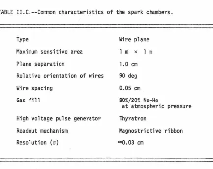
detection of at least one spark at each station. The efficiency of

individual chambers ranged from 90% to 99%. All chambers were of the

same physical size and the same basic design. We give their corrmon

characteristics in Table II.C.

TABLE II.C.--Co11TOon characteristics of the spark chambers.

Type

Maximum sensitive area

Plane separation

Relative orientation of wires

Wire spacing

Gas fill

High voltage pulse generator

Readout mechanism

Resolution (a)

Wire plane

l m x l m

1.0 cm

90 deg

0.05 cm

80%/20% Ne-He

at atmospheric pressure

Thyratron

Magnostrictive ribbon

~0.03 cm

To minimize the eccurrence of extraneous sparks in the chambers we

33 II.4

chamber and the spectrometer magnet. We simply severed the connection

of chamber wires with their bus bar. By the same technique we deadened

vertical bands through which the beam traversed the YZ chambers at

stations 1, 2, and 3. At station 4 the beam traversed a gap between

chamber pairs YZ7,8 and YZ9,10. To deaden the beam-illuminated area

of the UV chambers we inserted slabs of polyurethane foam between the

wire planes.

The physically relevant parameters of a forward scattered

track are its momentum and the scattering angle. For fixed values of

only these parameters some trajectories successfully negotiate the

spectrometer while others miss an aperture or traverse the dead region

at one of the stations. The resulting detection probability depends

heavily both on the momentum and the scattering angle, and we must

account for it in the analysis of the data. We discuss this issue in

detail in Section IV.5.

The most important measurement which the spectrometer supplied

was the bend angle in the magnet. The resolution (cr) for this

measure-ment was 0.25 mrad. The contributions from position error of the spark

chambers and from multiple scattering in the chambers and intervening

material were nearly equal. The relation of momentum to bend angle is

p

14 GeV

=

62 mrad

e

From this follows the relation for the error of the momentum.

34 II.4

6P

=

p2 68

14 GeV 62 mrad

(4.2)

=

P2 x 2.9 x l0-4 Gev- 1 6P is ~60 MeV at 14 GeV and ~30 MeV at 10 GeV. 5. Triggering and the Role of the Online Computer

The logic equation for the spark chamber trigger signal was

SCTRIG

=

GATE•(Rl + Ll)•(R3 + L3) (5.1)

The factor GATE was true for the duration of every beam pulse. The

SCTRIG signal was fanned out to the high voltage pulse circuits at

each chamber. Because of cable delays and the rise time of the HV

pulsers, sparks developed roughly 0.4 µsec after the triggering particle

traversed the spectrometer. The memory time of the chambers easily

acco1T111odated this delay. Because of the delay, however, and because the

beam 11

spill11

was so short, a second track was sometimes observable in

the spark chambers.

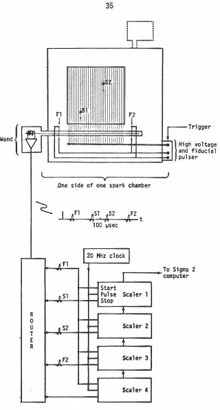
Figure 9 shows schematically the electronics used to

digitize spark coordinates. We use the term "wand" to refer to a

magnetostrictive ribbon, its mechanical support, the pickup coil, and

integral preamp. Near the ends of each wand at precisely known

loca-tions on the chambers were fiducial wires. Synchronously with the

I

-9

-~

l

<_

R 0

u T

E

R

35

J~

Fl

1111

I

,... _{lii!ll!I i:}1 .I _{1 .!il!li} I

lll!illii!iiii i!!lll!lilllll

v

·

-

-··

.

t

.

I

.

t

.

I

t I

I I

t I

-.. t

---

I

-

·

t I

F2

I

-I

.One side of one spark chamber

I {l

"' ;.s1. ₁₀₀ J.5_µsec 2 '"

l

2

t

A Fl

I

20 MHz clock

I

~-I

Start

n Sl

-

Pulse Scaler 1 Stop

'

ft S2

-

Scaler 2

t

II F2

-

Scaler 3

t

-

Scaler 4

~

and

~. pul

J

Trigger

h voltage fiducial ser

To Sigm compute

a 2

r

II. 5

FIG. 9. Schematic of the spark digitizing electronics. Fl and F2 are

36 11.5

initiated acoustic pulses in the magnetostrictive ribbon. Because the

acoustic pulse propagates along the ribbon with uniform velocity, the

position of the source of a pulse corresponds to a time of arrival at

the pickup coil. The first fiducial pulse from a wand started four

20 MHz 12 bit scalers associated with that wand. Succeeding pulses

stopped the scalers one by one. The last one to stop digitized the

time of arrival of the second fiducial except on occasion when a

chamber produced more than three sparks. The computer maintained a

running average of the digitizations obtained for the fiducial, and

this average established the effective propagation velocity in the

magnetostrictive ribbon.

We developed computer codes for the online Sigma 2 computer to

perform three primary tasks. One was to fetch the spark coordinates

from the spark chamber electronics and to record these on magnetic

tape. A second was to do some minimal analysis of the data to ensure

that the spectrometer was functioning satisfactorily. The third task,

and the most noteworthy, was to select pulses on which to trigger the

bubble chamber flash tubes. The design of this algorithm required

great care so as to satisfy the 3 msec time constraint.t

The trigger algorithm deals with the reaction

(5.2)

37 II.5

The system X includes one nucleon and an arbitrary number of mesons.

The primary objective is to generate a trigger when X includes at

least one pion. The cross section for elastic scattering is about a

factor of three larger than the cross section for the dissociation·

reactions which we seek to study. An algorithm must identify elastics

with efficiency greater than 93% in order that contamination of the

triggers be less than 20%.

We use the notation Mp' Mx for the masses of the proton and

X, and we use Pb and Pf for the magnitude in the lab frame of the

momenta of the beam particle, nb , and the secondary particle measured

in the spectrometer, nf • Neither of these momenta is ever less

than 6.5 GeV. For this discussion we can safely approximate the energies

of the pions by their momenta. Conservation of 4-momentum in the

reaction yields an expression for M; •

with t the square of the 4-momentum transfer from nb to nf An

adequate approximation for t is

¢y and ¢z are the vertical and horizontal projections of the

scattering angle.t

tProjecting an angle in this way is also an approximation which is satisfactory for our scattering angles of ~ 60 mrad.

38

We determine Pf from its bend angle in the spectrometer

according to the relation

11.5

{5.5)

The right hand side is the integral of the y component of the magnetic

field over the trajectory through the spectrometer magnet. We can

approximate this integral by the sum of the dipole term and a sextupole

term.

{5.6)

P

0 is the design momentum of the beam, and e0 is the bend angle of

an on-axis pion with this momentum. The quantities dz and dy are

the horizontal and vertical displacements of the trajectory from the

x axis of the magnet. The coefficient b is positive with magnitude

about l.lxl0- 5 cm-2 for the magnet. In analogy with the angle ef we

may define the angle eb which is the bend angle that the spectrometer

would measure for a beam track.

{5.7)

39 II.5 the average, eb , by using a small dipole magnet upstream of the bubble

chamber to steer the beam, at reduced intensity, into the active area

of the spark chambers.

We now combine relations (5.3)-(5.7) to obtain

- d2) p p ( 2 + 2)

y - b f ¢y ¢z

{5.8)

In a loose approximation which ignores the dimensions of the beam and

the bubble chamber we can write

(5.9)

xM is the distance from the bubble chamber to the spectrometer magnet.

Using relations

(5.9)

in a rearrangement of equation

(5.8)

we have

(5.10)

wherein

Cy

=

_{2 MpbxM - Pb} 2

=

-4 GeV (5.11)

c

_t

.

=

₂

Mpbx~

+ Pb

=

24 GeV . (5.12)

40 II.5

the z coordinates of the sparks. This information is sufficient to

compute only the first and second terms on the right hand side of

equation (5.10). The second term may be as large as 1.0 Gev2, and

neglecting it in the trigger·program would have resulted in too much

contamination from elastic scatters. Because of the dimensions of the

magnet aperture, the maximum value of ¢y is about one half the

maximum of ¢z . On this account and because ICyl << ICzl , the third

term in equation (5.10) is

~0.08

GeV2 • Since the threshold in

M~

-

M~

for single pion production is 0.28 GeV2 , neglect of the

third term in the trigger creates no difficulties.

In Appendix A we describe in detail the steps taken by the

trigger program to identify tracks corresponding to inelastic events.

In Figure 10 we show a histogram of the time required for the trigger

program to reach a decision. For a small fraction of the spark chamber

triggers,the trigger program required more than 3 msec to conclude.

In these cases if the program called for a picture, the picture was

lost. In Table II.D we give statistics of the data acquisition and

L{")

C\1

0

a::; w

0..

a::; w

CD

:E

:::::>

z

1000

500

41

TIME TO TRIGGER DECISION

5720 ENTRIES

~3%

o late

OL-~-'-~---1~.J___._~__L~~-L-~_J_~~t=:::::l 0

r

Beam Data in

l

computer

2

TIME IN MSEC

3

f XBL 774-8563

Light flash time

FIG: 10. Distribution of the time required for the trigger program to reach its decision.

TABLE II.D.--Statistics of data collection. Number As a fraction of acquired Beam pulses SC triggers BC pictures BC events Beam pulses 5.5xl0 6 Spark chamber triggers 2.5xl0 6 0.45 BC picture triggers 3.2x10 5 0.058 0.13 Pictures lost because 1. Ox10 4 of late trigger 0.002 0.004 0.03

~ N

BC triggers on events l. lx10 5 in fiducial volume 0.020 0.044 0.34 BC triggers on 2.8xl0 4 elastic scatters 0.0051 0.011 0.088 0.25 BC triggers on 4.9xl0 4 inelastic two prongs 0.0089 0.020 0.15 0.45 BC triggers on 3. 5xl0 4 four prongs 0.0064 0.014 0.11 0.32 BC triggers on

-+ 1. 7xl0 4 0.0031 0.0068 0.053 0.15 np-+nnnp

43

II I. PROCESS ING

1. Overview

We describe in this _chapter the metamorphosis of the data from

its original state to a form convenient for study of its physics, For

75% of the film all processing took place at Lawrence Berkeley

Labora-tory. For the remaining 25% Caltech carried out the scanning and

measuring on systems quite different from the LBL apparatus. In this

report we will describe only the LBL processing, and we will use only

LBL processed data in the analysis of the next chapter.

In Figure 11 we show schematically the major processes and

trace the flow of information from one to another. The figure is only

illustrative since large segments of the film received treatment which

varied in some respect from what is shown. For example some rolls did

not undergo filtering, and the measurement of other rolls was

exclu-sively via COB\1EB. In the last section of the chapter we discuss one

of the tests that we made to verify correct operation of the processes

from measurement through fitting.

2. Processing of the Spark Chamber Data

Our raw spark chamber data for an event consisted of groups of

spark digitizations associated with each coordinate of each chamber.

A computer code which we built and named TORTIS reorganized the

digi-tizations into "track banks." The collection of sparks forming a track

bank defined a trajectory which a charged particle could have followed

44

0

Bubble chamber film _{recorded on magnetic tape} Spectrometer data

Scanning

Filtering (SCMATCH)

FSD measurement

COBWEB measurement

Track finding

- - - 1 (TORTIS)

Geometrical

reconstruction 1 - - - - .

(TVGP)

Hybridization (HYBRID)

Kinematic fitting {SQUAW)

I I

r---1----~,

I

Event selection

I

1 and analysis for I

I

individual channels

I

L _ ...!

III.2

45

track banks for each event, and it permitted each digitization to

appear in an arbitrary number of banks. The TORTIS algorithm went

roughly as follows. (y and z are defined in Figure 8.)

III.2

1) Merge the sparks of adjacent chambers into station banks

and remove redundant sparks.

2) Find all sets of four z coordinates, one from each

station, for which the lines defined by the station 1,2 pair and the

station 3,4 pair intersect at the midplane of the spectrometer magnet.

A separation of the lines at the midplane of less than 0.3 cm satisfies

this condition.

3) Analogously find sets of four y coordinates, one from

each station, but additionally require that the angle between the lines

be less than 2.5 mrad. The tolerance on this angle accormnodates the

bend in the vertical plane caused by the fringe field of the

spectro-meter magnet.

4) Pair each set of y coordinates with each set of z

coordinates. When the UV chambers at station l contain digitizations

consistent with the y,z position, fonn a track bank. In the case that

steps 2 and 3 result in just one z coordinate set and one y set,

fonn the track bank regardless of the UV chamber output.

The tolerances used in TORTIS were liberal enough that the

algorithms did not add significantly to the inefficiency of the spark

chambers themselves. Considering only those beam pulses which generated

a BC camera trigger, the TORTIS efficiency was at least 95%. The

precise value is unimportant because it does not enter in the method

46

created by TORTIS were available to the filter and hybridization

processes which we describe in succeeding sections.

3. Scanning and Filtering

III.2

Bona fide events occurring within the fiducial volume of the

bubble chamber (70 cm in length) account for only 35% of the BC camera

triggers. The balance are ascribable to events occurring in hydrogen

outside the fiducial volume (58 cm, much of which was invisible), to

events occurring in the beam entrance and exit windows (equivalent to

18 cm of H2), and to decays of beam particles in the last several meters of beam preceding the station 1 spark chambers. A typical roll

of film of 1000 frame~ containing ~50 bona fide events, contains in

addition ::::::350 events within the fiducial volume which are not trigger

associated and do not match a track in the spectrometer. Measurement

of these interlopers is unproductive, so we devised a scanning process

which substantially reduced this burden.

Our scanners worked at scan tables equipped wih an image plane

digitizing arm electronically interfaced to a magnetic tape drive. When

they located an event, they digitized one fiducial and the vertex of

the event in one view only. By the touch of a button the scanner

recorded the roll and frame numbers, the event type, and the

digitiza-tions. We used this procedure to locate all events except those with

kinks or V's resulting from the production and decay of strange particles.

The scan output and the TORTIS output were the input to a

47 III.3

code projected each of the spectrometer tracks back to the x

coordi-nate of the event's vertex. When the y coordicoordi-nate of the vertex was

within 1.8 cm of one of the projections, the code flagged the event for

measurement. We adopted the generous 1.8 cm tolerance rather than take

pains to optimize this process. The output per 1000 frames contained

all trigger associated events and ~go interlopers. The 25% extra measurement burden was acceptable.

4. Measuring

We utilized two independent systems for measuring the events.

One was a flying spot digitizer, FSD (known in some quarters as a

Hough-Powel l device, HPD) under the control of an IBM 7094 computer [White et

al. 1968]. Its mode of operation was fully and exclusively automatic;

it had no provision for operator assistance in the measurement process.

We will give no further details of this system.

The second system, called COBWEB [Albrecht et al. 1968],

con-sisted of several film plane digitizing engines. known as Frankensteins,

interfaced to an IBM 7044 computer. The control electronics of the

Frankensteins made them "semiautomatic." The reticle of the device is

an orientable slit. So long as the operator maintains the axis of

the slit within 6° of the tangent to a track, the electronics will

drive the stage so that the track passes precisely through the center

of the reticle. The machine can automatically digitize at intervals

along the track while the stage is in motion. Completely manual control

48 III.4

regions of confusion or obstruction of a track. The computer as well

as the operator can control stage position and frame advance, and the

computer intervenes where possible to speed the measurement process.

The FSD system was the first to process each roll. It produced

measurements for about 45% of the events on the measurement list. We

then directed the COBWEB system to measure those events (55%) on which

the FSD system failed. The output of either system was a magnetic tape

record containing up to twenty pairs of film plane digitizations for

each view of each track.

5. Geometrical Reconstruction

The input to the process which we call reconstruction is the

output of the measuring systems just described. Its function is to

produce a five parameter description of each track and the 5x5 error

matrix for the parameters, Specifically, in the coordinate system of

Figure 8 , the parameters are the polar and azimuthal angles and

the curvature at the beginning of the track, and the polar and azimuthal

angles at the end of the track. The computer code which we utilized for

reconstruction was TVGP (Three View Geometry Program) [Solmitz et al.

1966]. This code has seen prior use in many experiments and with

several different bubble chambers and measurement systems. Its

archi-tecture facilitates adaptation to a particular bubble chamber, and we

had only to ~evelop the necessary modifications for the SLAC 40"

chamber.

49 III.5

mass as well as momentum because of energy loss by ionization, dE/dx.

TVGP obligingly allows for a number of different mass interpretations

of each track. For negative tracks we obtained only a w-

interpreta-tion, and for positive tracks we obtained the TI+ and proton

interpre-tations. We omitted K~ and K+ interpretations and other more

esoteric possibilities in favor of savings in computer charges.

6. Hybridizatton

We built a computer code, HYBRID, which amalga