R E S E A R C H
Open Access
Experimental study of image representation
spaces in variational disparity calculation
Jarno Ralli
*, Javier D´ıaz, Pablo Guzm´an and Eduardo Ros
Abstract
Correspondence techniques start from the assumption, based on the Lambertian reflection model, that the apparent brightness of a surface is independent of the observer’s angle of view. From this, a grey value constancy assumption is derived, which states that a change in brightness of a particular image pixel is proportional to a change in its position. This constancy assumption can be extended directly for vector valued images, such as RGB. It is clear that the grey value constancy assumption does not hold for surfaces with a non-Lambertian behaviour and, therefore, the underlying image representation is crucial when using real image sequences under varying lighting conditions and noise from the imaging device. In order for the correspondence methods to produce good, temporally coherent results, properties such as robustness to noise, illumination invariance, and stability with respect to small geometrical deformations are all desired properties of the representation. In this article, we study how different image
representation spaces complement each other and how the chosen representations benefit from the combination in terms of both robustness and accuracy. The model used for establishing the correspondences, based on the calculus of variations, is itself considered robust. However, we show that considerable improvements are possible, especially in the case of real image sequences, by using an appropriate image representation. We also show how optimum (or near optimum) parameters, related to each representation space, can be efficiently found.
Introduction
The optical flow constraint [1], based on the Lambertian reflection model, states that a change in the brightness of a pixel is proportional to a change in its position, i.e., the grey level of a pixel is assumed to stay constant tem-porally. This same constancy concept can be used also in disparity calculation by taking into account the epipolar geometry of the imaging devices (e.g., a stereo-rig). The grey level constancy, that does not hold for surfaces with a non-Lambertian behaviour, can be extended for vec-tor valued images with different image representations. In this study, we use a method based on the calculus of variations for approximating the disparity map. Vari-ational correspondence models typically have two terms, the first one being a data term (e.g., based on the grey level constancy), while the second one is a regularisation term used to make the solution smooth. In order to make the data term more robust with respect to non-Lambertian
*Correspondence: jarno@ralli.fi
Departamento de Arquitectura y Tecnolog´ıa de Computadores, Escuela T´ecnica Superior de Ingenier´ıas y de Telecomunicaci ´on, Universidad de Granada, Calle Periodista Daniel Saucedo Aranda s/n, E-18071 Granada, Spain
behaviour, different image representations can be used. Some of the problems in establishing correspondences arise from the imaging devices (e.g., camera/lens parame-ters being slightly different, noise due to imaging devices) and some, from the actual scene being observed (e.g., lighting conditions, geometrical deformations due to cam-era setup). Typically, illumination difference and optics related ‘errors’ are modelled as a multiplicative type of error, while the imaging device itself is modelled as a com-bination of both multiplicative and additive ‘errors’. It is clear that the underlying image representation is crucial in order for any correspondence method to generate correct, temporally coherent estimates in ‘real’ image sequences.
In this article, we study how combinations of differ-ent image represdiffer-entations behave with respect to both illumination errors and noise, ranking the results accord-ingly. We believe that such information is useful to the part of the visual community that concentrates on appli-cations, such as obstacle detection in vehicle related sce-narios [2], segmentation [3], and so on. Although other authors address similar issues [4,5], we find these to be slightly limited in scope due to a reduced ‘test bench’,
e.g., a small number of test images or image representa-tions. Also, in most of the cases, the way in which the parameters related to the model(s) have been chosen is not satisfactorily explained. Therefore, the main contri-bution of our article is an analysis of the different image representations supported by a more detailed and sys-tematical evaluation methodology. For example, we show how optimum (or near optimum) parameters for the algo-rithm, related to each representation space, can be found. This is a small but important contribution in the case of real, non controlled, scenarios. The standard image rep-resentation is the RGB-space, the others being (obtained via image transformations): gradient, gradient magnitude, log-derivative, HSV, rφθ, and phase component of an image filtered using a bank of Gabor filters.
This work is a comparative study of the chosen image representations, and it is beyond the scope of this arti-cle to explain why certain representations perform better than others in certain situations. Under realistic illumi-nation conditions, with surfaces both complying and not complying with the Lambertian reflection model, theoret-ical studies can become overly complex, as we show next. It is typically thought that chromaticity spaces are illumi-nation invariant, but under realistic lightning conditions, this is not necessarily so [6]. One of the physical models that explains light reflected by an object is the Dichro-matic Reflection Model [7] (DRM), which in its basic form assumes that there is a single source of light [7], which is unrealistic in the case of real images (unless the light-ning conditions can be controlled). A good example of this is given by Maxwell et al. in their Bi-Illuminant Dichro-matic Reflection article [6]: in a typical outdoor case, the main illuminants are sunlight and skylight, where fully lit objects are dominated by sunlight while objects in the shade are dominated by skylight. Thus, as the illumina-tion intensity decreases, the hue of the observed colour becomes bluish. For the above mentioned reasons, chro-matic spaces (e.g., HSV,rφθ) are not totally illumination invariant under realistic lightning conditions. Therefore, in general, we do not speak of illumination invariance in this article but of illumination robustness or robust image representation with respect to illumination changes and noise. By illumination error, we refer to varying illu-mination conditions between the left- and right stereo cameras.
Next, Section 1 presents the relevant related study, some sources of error, and the variational method. Finally, in Sections 1, 1, and 1, we describe the proposed methodolo-gies, results, and conclusions.
Background material and related study Related study
The idea of robust ‘key-point’ identification is an impor-tant aspect of many vision related problems and has
lead to such concepts as SIFT [8] (scale invariant fea-ture transform) or SURF [9] (speeded up robust feafea-tures). This study relates to identifying robust features as well, however, in the framework of variational stereo. Several studies comparing different data- or smoothness terms for optical-flow exist, for example, those of Bruhn [10] and Brox [11]. A similar study to the one presented here, carried out in a smaller scale for the optical-flow, has been done by Mileva et al. [4]. On the other hand, in [5], W¨ohler et al. describe a method for 3D reconstruc-tion of surfaces with non-Lambertian properties. How-ever, many comparative studies do not typically explain in detail how the parameters for each different competing algorithm or representation were obtained. Also, some-times it is not mentioned, if the learn and test sets for obtaining the parameters were the same. This poses prob-lems related to biasing and over-training. If the param-eters have been obtained manually, they are prone to bias from the user: expected results might get confirmed. On the other hand, if the learn and test sets were the same or they were too small, it is possible that over-training has taken place and, therefore, the results are not generalisable. We argue that in order to properly rank a set of representation spaces or different algo-rithms, with respect to any performance measure, opti-mum parameters related to each case need to be searched consistently, with minimum human interference, avoiding over-fitting.
Where our study differs from the rest is that (a) we use an advanced optimisation scheme to automatically opti-mise the parameters related to each image representation space, (b) image sets for optimisation (learning) and test-ing are different in order to avoid over-fitttest-ing, (c) we study the robustness of each representation space with respect to several image noise and illumination error models, and (d) we combine the results for both noise and illumina-tion errors. Thus, the methodology can be considered to be novel.
Sources of error
shadow cast upon a moving object makes it more difficult to find the corresponding pixels. Also, as it was already mentioned in Section 1, the imaging devices also cause problems in the form of noise, motion blur, and so on. Thus, an image representation space should be robust with respect to (a) small geometrical deformations (geo-metrical robustness), (b) changes in the illumination level (illumination robustness), both global and local, and (c) noise present in the images (e.g., due to the acquisition device). Our analysis was carried out for stereo but is directly applicable to optical-flow as well.
Variational stereo
We have chosen to use a variational method for several different reasons: (a) transparent modelling of the corre-spondence problem; (b) extending the model is straight-forward; (c) the same mathematical formalism can be used for both optical-flow and stereo; and (d) the governing differential equation(s) can be solved efficiently [12]. The original idea of solving optical-flow in a variational frame-work is by Horn and Schunck [1]. The particular method that we have used was introduced by Slesareva et al. in [13] and is based on the optical-flow method of Brox et al. [14]. The characteristics of this method are: error functions for both the data and the regularisation terms are quadratic [14,15]; the regularisation term is non-linear isotropic [12,16], based on the flow (flow-driven) and warping over several scales (multi-resolution strat-egy) is used in order to recover greater displacements with late linearisation [14,17,18] of the constancy terms. A Matlab/MEX code of the algorithm can be downloaded froma.
Before going any further, we introduce the used nota-tion, so that the rest of the text would be more readable.
Notation
We consider the (discrete) image to be a mappingI(x,k):
→ RK+, where the domain of the image is :=
[ 1,. . .,N]×[ 1,. . .,M], M and N being the number
of columns and rows of the image, K defines number
of the channels, and x = (x,y). In our case K = 3, since the input images are RGB, that is, I(x,k) := [R(x) G(x) B(x)]. The input image is then transformed into the desired image representation by I(x,k) →
T(x,kt)so thatT(x,kt) : → RKT+, whereKT is the number of channels of the transformed image andis as defined previously. We use subindicesLandRto refer to the left- and the right images. Superindexwmeans that the components in question are ‘warped’ using the dis-parity d. For example, TRw = Tx+ d(x,y),tR means that all the components of the right image are warped as per disparity d = d(x,y). For ‘warping’ we use bilinear interpolation.
Model
The energy functional to be minimised is as follows:
E(d)=
2
t=1
btDt(TL,TR,d)
dx+α
S(∇d)dx
E(d)=
⎛
⎝b1D1(TL,TR,d)+b2D2(TL,TR,d)
combined data term
⎞ ⎠dx
+α
S(∇d)dx
(1)
whereD1(IL,IR,d)andD2(IL,IR,d)are components of the combined data term,S(∇d)is the regularisation term, and T{L,R}refers to the transformed versions of the left and the right images (all the channels).b1≥0,b2 ≥0 andα≥0
are the parameters of the model, defining the weight of the corresponding term. Both the data and the regularisation terms are defined as:
Dt(TL,TR,d):= KT
kt=1
TL,kt−TRw,kt
2 2
, ∀t
S(∇d):=∇d22
(2)
whereTL,kt = T
x,y,ktLis thektth channel of the left transformed image,TRw,kt=Tx+d(x,y),y,ktRis thektth channel of the right transformed image warped as per dis-parityd = d(x,y),(s2) = √s2+2is a non-quadratic
error function, and · 2 is theL2 norm. For ‘warping’
we use bilinear interpolation. We would like to point out that even if formal definitions for all the Dt are ‘equal’, the used image representation (i.e., transformation) is not necessarily the same for each t. We could have used an additional index for pointing out this fact, but we feel it should be clear from the context.
Because of the ambiguities related to the different rep-resentations and the L2 norm, here we give a concrete
example of (2) for the∇I(see 1) and|∇I|(see 1) repre-sentations. More specifically, we use∇Irepresentation for D1and|∇I|forD2. For clarity’s sake, we refer directly to
the channels R, G and B, while subindices{L,R}indicate which image (left or right) is in question. Terms of the∇I representation are:
∇IL:=
∂RL ∂x
∂RL ∂y
∂GL ∂x
∂GL ∂y
∂BL ∂x
∂BL ∂y
∇IR:=
∂RR ∂x
∂RR ∂y
∂GR ∂x
∂GR ∂y
∂BR ∂x
∂BR ∂y
,
whereas terms of the|∇I|representation are:
|∇IL|:= ∂RL ∂x
∂RL ∂y
∂GL ∂x
∂GL ∂y
∂BL ∂x
∂BL ∂y
|∇IR|:= ∂RR ∂x
∂RR ∂y
∂GR ∂x
∂GR ∂y
∂BR ∂x
∂BR ∂y
(4)
In the (4) case the inner brackets (i.e., [·]) are used to indicate over which terms the norm is calculated. In other words, in (3)KT=6, whereas in (4)KT =3. Next step is to ‘plug’ terms of each representation into Equation (2) in order to get the actual data terms. For the∇Iwe have:
D1(∇IL,∇IR,d)=
∂RL
∂x − ∂RwR
∂x 2 + ∂RL ∂y − ∂RwR
∂y 2
+
∂GL
∂x − ∂Gw R ∂x 2 + ∂GL ∂y − ∂Gw R ∂y 2 +
∂BL
∂x − ∂Bw R ∂x 2 + ∂BL ∂y − ∂Bw R ∂y 2 (5)
The same for the|∇I|is:
D2(|∇IL|,|∇IR|,d)=
∂RL ∂x − ∂Rw R ∂x 2 + ∂RL ∂y − ∂Rw R ∂y 2 + ∂GL ∂x − ∂Gw R ∂x 2 + ∂GL ∂y − ∂Gw
R ∂y 2 + ∂BL ∂x − ∂Bw R ∂x 2 + ∂BL ∂y − ∂Bw R ∂y 2 (6)
where the superindexwrefers to warping as previously, i.e.,TRw,kt=Tx+d(x,y),y,ktR. In order to complete the example, using the above mentioned representations, the complete energy functional would be written as:
E(d)= b1 ∂RL
∂x − ∂RwR
∂x 2
+b1
∂RL
∂y − ∂RwR
∂y 2
+b1
∂GL
∂x − ∂Gw
R
∂x 2
+b1
∂GL ∂y − ∂Gw R ∂y 2
+b1
∂BL
∂x − ∂Bw
R
∂x 2
+b1
∂BL ∂y − ∂Bw R ∂y 2
+b2
∂RL
∂x − ∂Rw R ∂x 2 + ∂RL ∂y − ∂Rw R ∂y 2
+b2
∂GL
∂x − ∂GwR
∂x 2
+∂GL
∂y − ∂GwR
∂y 2
+b2
∂B
L
∂x − ∂BwR
∂x 2 + ∂B L ∂y − ∂BwR
∂y 2 dx +α ∇d2
2
dx
(7)
As we can see from Equations (5) and (6), error func-tion (·) acts differently for ‘scalar’ and ‘vector’ fields. In (5), each of the components has its own error func-tion, while in (6), the components are ‘wrapped’ inside the same error function. In order to have a better insight how this affects robustness, let us suppose that at a given posi-tion, the vertical derivative could not approximated well and, thus, would be considered an outlier. In the∇Icase, only the vertical derivative would be suppressed (i.e., the component considered an outlier), while the horizontal derivative would still be used for approximating the dis-parity. In the|∇I| case, however, the whole term would be suppressed and the horizontal derivative would not be used either for approximating the disparity.
Now, with both the energy functional and the related data terms described, a physical interpretation of the model can be derived: we are looking for a transformation described bydthat transforms the right image represen-tation into the left image represenrepresen-tation, with thedbeing piecewise smooth. By transforming the right image into the left image, we mean that the image features described by the data term(s) align.
Since the model is well known, we only quickly cover its characteristics. A quadratic error function typically gives too much weight to outliers, i.e., where the data does not fit well with the model. In the data term case, these outliers arise from where the Lambertian reflec-tion model does not accurately describe surfaces of the objects being observed or from occluded regions (i.e., fea-tures seen only in one of the images). On the other hand, in the case of the regularisation term, outliers are those approximations that do not belong to the surface in ques-tion and, thus, regularisaques-tion across object boundaries belonging to different surfaces takes place. The use of a non-quadratic error function [15] makes the model more robust with respect to the outliers. In the case of the regu-larisation term, this means that the solution is piece-wise smooth [16,17]. As can be observed from (2), each chan-nel in both data terms has its own penalisation function (s2+2)[19]. Since the error functions are now sepa-rate, this implies that if one of the constancy assumptions is rejected due to an outlier, other channels can still gen-erate valid estimations, thus increasing the robustness of the method. Theoretically, any number of different rep-resentations could be used in the data term, but we have limited the number to two in this work in order to keep the computational cost at a reasonable level.
Solving the equations
linearisation of the data term is postponed until discreti-sation of rest of the terms [12,14,17,18]. Because of late linearisation, the model has the benefit of coping with large displacements, which, however, comes at a price: the energy functionals are convex. Due to the non-convexity, many local minima possibly exist and, there-fore, finding a suitable relevant minimiser becomes more difficult. Another difficulty is due to the non-linearity of the robust error function. One such way of finding a rel-evant minimiser are the so called continuation methods (e.g., Graduated Nonconvexity [20]): search for a suitable solution is started from a simpler, smoothened version of the problem which is used to initialise the search at a finer scale. This is also known as a coarse-to-fine resolution (or multigrid) strategy [12,14,18,21]. The multi-resolution strategy has two very important implications that are interconnected. First, this means that the solu-tion to the partial differential equasolu-tion (PDE) is searched using a multigrid technique which has a positive effect on the convergence rate [12,21]. Second, the problem of physically irrelevant local minima is also efficiently over-come by the this scheme: a solution from a simplified version of the problem (coarse scale) is used to initialise the next finer scale [12,18]. While this does not guarantee that a global minimiser is found, it does, however, pre-vent getting stuck on a non-relevant local minimum [20]. In order to deal with the non-linearities, a lagged diffusiv-ity fixed point method is used [10,11]. The solver used for the linearised versions of the equations is alternating line relaxation (ALR) which is a Gauss-Seidel type block solver [10,21].
Proposed methodologies
Searching for optimal parameters with differential evolution
Since the main idea of this study is to rank the cho-sen image reprecho-sentation spaces with respect to robust-ness, we have to find an optimum (or near optimum) set of parameter vectors [b1b2α] for each different case,
avoiding over-fitting. As was already mentioned, using a human operator would be prone to bias. Therefore, we have decided to use a gradient free, stochastic, population based function minimiser called differential evolutionb (DE) [22,23]. The rationale for using DE is that it has empirically been shown to find the optimum (or near optimum), it is computationally efficient, and the cost function evaluation can be efficiently parallelised. The principal idea behind DE is to represent the parameters to be optimised as vectors where each vector is a pop-ulation member whose fitness is described by the cost function value. A population at timetis also known as a generation. Therefore, it can be understood that the sys-tem evolves with respect to artificial timet, also known as cycles. By recurring to the survival of the fittest theorem,
the ‘fittest’ members contribute more to the coming pop-ulations and, thus, their characteristics overcome those of the weak members, therefore minimising (or maximising) the function value [22,23]. Two members (parents) are stochastically combined into a new one (offspring), possi-bly with mutation, which then competes against the rest of the members of the coming generations. Therefore, in our case, a single member is a vector given by [b1b2α] while
the cost function value is the mean squared error (MSE) given by Equation (31).
In order to compare the results obtained using differ-ent combinations of the image represdiffer-entations, we adopt a strategy typically used in pattern recognition: the input set (a set of stereo-images) is divided into a learning, a validation, and a test set. The learning set is used for obtaining the optimal parameters while the validation set is used to prevent over-fitting: during the optimisation, when the error for the validation set starts to increase, we stop the optimisation process, therefore keeping the solu-tion ‘general’. This methodology is completely general and can be applied to any other image registration algorithm with only some small modifications. DE itself is compu-tationally cost efficient, the problem being that several function evaluations (one per population member) per cycle are needed. The following table displays the parame-ters related to the DE, thus allowing us to approximate the computational effort.
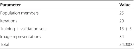
From Table 1, we can see that a total of 34,0000 cost function evaluations are done in order to find the param-eters. On the average, each cost function evaluation takes approx. 5 s (Matlab/MEX implementation). Therefore, it would take around 19.7 days ‘wall clock time’ to find the parameters. As is explained in Section 1, we repeat this procedure 5 times. However, the optimisation can be par-allelised by keeping the members on the master computer and by calculating the function values on several slave computers simultaneously, which was the adopted strat-egy. This method of parallelising DE is certainly not new and has been reported earlier by, for example, Plagianakos et al. [24], Tasoulis et al. [25], and Epitropakis et al. [26]. The whole system was implemented on a ‘Ferlin’ LSF-type cluster (Foundation Level System) at the PDC Center for High Performance Computing, KTH, Stockholm, Sweden. The cluster consists of 672 computational nodes (each
Table 1 DE parameters
Parameter Value
Population members 25
Iterations 20
Training+validation sets 15+5
Image representations 34
node consists of two quad-core Intel CPUs). By using four computational nodes (i.e., 32 cores), the total ‘wall clock time’, for all the five different runs (see Section 1), was approximately 5 days.
Image transformations
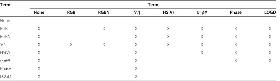
In this section, we describe the image transformations that we have decided to evaluate. We have chosen the most common image representations as well as other transfor-mations that have been proposed in the literature, due to their robustness and possibility of real-time implementa-tion. All combinatorial pairs of NONE, RGB, RGBN,∇I, HS(V),(r)φθ, PHASE, LOGD and|∇I|are tested, except |∇I|and PHASE+LOGD. The 34 different tested combi-nations can be seen in Appendix 1, Table 7. As it was already mentioned previously, Mileva et al. tested some of the same representations earlier in [4]. Some combina-tions were left out because of practical issues related to the computational time (see Section Searching for optimal parameters with differential evolution for more informa-tion related to the computainforma-tional time). A preliminary ‘small scale’ experiment was conducted in order to see which representations would be studied more carefully. In the following section, we briefly describe the different input representations under study.
RGBN (normalized RGB)
In the RGBN case, the standard RGB representation is simply normalised by using a factorN. In our tests, both images are normalised by using their own factor which is Ni = max(Ri,Gi,Bi), i being the image in question (e.g., left or right image). The transformation is given by Equation (8).
R G BT → R N G N B N T (8)
RGBN is robust with respect to global multiplicative illu-mination changes.
∇I
The transformation is given by:
R G BT →Rx Ry Gx Gy Bx By T
(9)
where sub-index states with respect to which variable the term in question has been derived. Gradient con-stancy term is robust with respect to both global and local additive illumination changes.
|∇I|
The transformation is given by:
[R G B]T →[Rx Ry] [Gx Gy] [Bx By] T
(10)
where sub-index states with respect to which variable the term in question has been derived. In general, this term is illumination robust with respect to both local and global additive illumination changes.
HS(V)
HSV(Hue saturation value) is a cylindrical representation of the colour-space where the angle around the central axis of the cylinder defines ‘hue’, the distance from the central axis defines ‘saturation’, and the position along the central axis defines ‘value’ as in:
R G B T →H S VT
H= ⎧ ⎪ ⎪ ⎪ ⎪ ⎪ ⎪ ⎪ ⎪ ⎪ ⎨ ⎪ ⎪ ⎪ ⎪ ⎪ ⎪ ⎪ ⎪ ⎪ ⎩
0, if max=min
60◦× G−B
max−min, if max=R
60◦× B−R
max−min +120
◦, if max=G
60◦× R−G
max−min +240
◦, if max=B
S= ⎧ ⎨ ⎩
0, if max=0
max−min
max , otherwise
V =max
(11)
where min = min(R,G,B)and max = max(R,G,B). As can be understood from (11), the H and S components are illumination robust, while the V component is not and, therefore, it is excluded from the representation. In the rest of the text, HS(V) refers to image representation with only the H and S components.
(r)φθ
While HSV describes colours in a cylindrical space,rφθ does so in a spherical one.rindicates the magnitude of the colour vector whileφis the zenith andθis the azimuth, as in:
R G BT →r θ φT
r=R2+G2+B2
θ =arctan
G R
φ=arcsin
√
R2+G2 √
R2+G2+B2
(12)
LOGD
With LOGD we refer to log-derivative representation and the corresponding transformation is as follows:
[R G B]T →[(ln R)x (ln G)x (lnB)x
×(ln R)y (ln G)y (ln B)y T
(13)
where sub-index states with respect to which variable the term in question has been derived. The log-derivative image representation is robust with respect to both addi-tive and multiplicaaddi-tive local illumination changes.
PHASE
The reason for choosing the phase representation is three-fold: (a) the phase component is robust with respect to illumination changes; (b) cells with a similar behaviour have been found in the visual cortex of primates [27], which might well mean that evolution has found this kind of representation to be meaningful (even if we might not be able to exploit it completely yet); and (c) the stability of the phase component with respect to small geometri-cal deformations (as shown by Fleet and Jepson [28,29]). The phase is a local component extracted from the sub-traction of local values. Therefore, it does not depend on an absolute illumination measure, but rather on the rela-tive illumination measures of two local estimations (which are subtracted). This makes this estimation robust against illumination artifacts (such as shadows, which increase or decrease local illumination but do not affect local ratios so dramatically). In a similar way, if noise (multiplicative or additive) affects a certain local region uniformly, in aver-age the illumination ratio (in which phase is based) will be less affected than the absolute illumination value. The fil-tering stage with a set of specific filters can be regarded as band-pass filtering, since only the components that match the set of filters are allowed (or not discarded) for fur-ther processing. Gabor filters have specific properties that make them of special interest in general image processing tasks [30].
We define the phase component of a band-pass fil-tered image as a result of convolving the input image
with a set of quadrature filters [28-30] as proceeds. The complex-valued Gabor filters are defined as:
h(x;f0,θ )=hc(x;f0,θ )+ihs(x;f0,θ ) (14)
wherex=(x,y)is the image position,f0denotes the peak
frequency,θthe orientation of the filter in reference to the horizontal axis, andhc(·)andhs(·)denote the even (real) and odd (imaginary) parts. The filter responses (band-pass signals) are generated by convolving an input image with a filter as in:
Q(x;θ )=I∗h(x;f0,θ )=C(x;θ )+iS(x;θ ) (15)
whereI denotes an input image, ∗denotes convolution, andC(x;θ ) andS(x;θ ) are the even and odd responses corresponding to a filter with an orientation θ. From the even and odd responses, two different representation spaces can be built, namely phase and energy as follows:
E(x;θ )=C(x,θ )2+S(x;θ )2
ω(x;θ )=arctan
S(x;θ )
C(x;θ )
(16)
where E(fx;θ ) is the energy response and ω(x;θ ), the phase response of a filter corresponding to an orienta-tionθ. As can be observed from (15), the input imageI can contain several components (e.g., RGB, HSV) where each component would be convolved independently to extract energy and phase. However, in order to maintain the computation time reasonable, the input images are first converted into grey-level images, after which the filter responses are calculated. Therefore, the transformation can be defined by:
[R G B]T →[ω(x;θ )] for allθ (17)
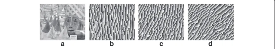
Figure 1 shows phase information for the Cones image from the Middlebury databasec.
Induced illumination errors and image noise
Here, we introduce, along with the related mathematical formulations, the used models for simulating both illumi-nation errors and image noise. Tables 2 and 3 display the error and noise models, in their respective order.
From Table 2, we can observe that both global and local illumination errors are used. The difference between these
Table 2 Tested illumination error types
Global Local
Additive (GA) Additive (LA) Multiplicative (GM) Multiplicative (LM)
Multiplicative and additive (GMA) Multiplicative and additive (LMA)
Table 3 Tested image noise types
Luminance Chrominance Salt & pepper
mild (nLM) mild (nCM) mild (nSPM) severe (nLS) severe (nCS) severe (nSPS)
types is that in the former case, the error is the same for all the positions, while in the latter, the error is a function of the pixel position. In the illumination error case (both local and global), we apply the error only on one of the images. Especially in the local illumination error case, this simulates a ‘glare’.
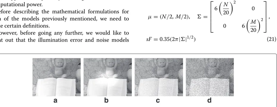
From Table 3, we can see that luminance, chrominance, and salt&pepper image noise types are used. The differ-ence between the luminance and the chrominance is that in the former case, the noise affects all the channels, while in the latter, only one channel is affected. We apply the noise model to both of the images (i.e., left- and right image). Figure 2 displays some of the illumination errors and image noise for the Baby2 case from the Middlebury databased.
It can be argued that the noise present in the images could be reduced or eliminated by using a de-noising pre-processing step, and thus, the study should be cen-tred more towards illumination type of errors. However, if any of the tested image representations proves to be suf-ficiently robust with respect to both illumination errors and image noise, this would mean that less pre-processing steps would be needed. This certainly would be beneficial in real applications, possibly suffering from a restricted computational power.
Before describing the mathematical formulations for each of the models previously mentioned, we need to make certain definitions.
However, before going any further, we would like to point out that the illumination error and noise models
are applied on the RGB input images before transform-ing these into the correspondtransform-ing representations. For the sake of readability, the used notation is explained here again. We consider the (discrete) image to be a mapping I(x,k) : → RK+, where the domain of the image is :=[ 1,. . .,N]×[ 1,. . .,M],MandNbeing the number of columns and rows of the image, while K defines the number of the channels. In our caseK=3, since the input images are RGB. Minimum and maximum values, after having applied the error or noise models, of the images are limited to [ 0,. . ., 255]. The position vector can be written as follows:x(i) = x(i),y(i), wherei ∈[ 1,. . .,P] withP being the number of pixels (i.e.,P = MN). When refer-ring to individual pixels, instead of writingI(x(i),k)), we writeI(i,k)withidefined as previously andkbeing the channel in question.
Global illumination errors
Global illumination errors are defined as follows:
GA:I(i, k)→I(i,k)+ga, (18)
GM:I(i,k)→I(i,k)gm, (19)
GMA:I(i, k)→I(i,k)gm+ga, (20)
where i = 1,. . .,P, k = 1,. . ., 3, and ga is the addi-tive error, whilegmis the multiplicative error. For additive error, we have usedga = 25 and for multiplicative error, we have usedgm=1.1.
Local illumination errors
We define the local illumination error function as a
map-ping E : → R, with the domain as previously. In
this study, we have used a scaled multivariate normal distribution, N2(x(i),μ,)sF, to approximate the local
illumination errors that change as a function of the posi-tion. Mean μ, covariance , and scaling factor sF are defined as follows:
μ=(N/2,M/2), = ⎡ ⎢ ⎢ ⎢ ⎣ 6
N 20
2
0
0 6
M 20
2
⎤ ⎥ ⎥ ⎥ ⎦,
sF=0.35(2π||1/2) (21)
where N andM are the number of columns and rows in the image (as previously) and || is determinant of the covariance. Scaling factorsF simply scales the values between [ 0,. . ., 0.35]. In other words, we simulate an illu-mination error that influences most the centre of the the image in question, as can be observed from Figure 2 (LMA case). With the above in place, we define the local illu-mination error function asEi := N2
x(i), μ,σsF and, thus, the local illumination errors are as follows:
LA:I(i,k)→I(i,k)+255E(i) (22)
LM:I(i,k)→I(i,k)
1+E(i)
(23)
LMA:I(i,k)→I(i,k)
1+E(i)
+255E(i) (24)
wherei = 1,. . .,Pandk = 1,. . ., 3. The multiplier 255 is simply due to the ‘scaling’ of the image representation (i.e., [ 0,. . ., 255]).
Luminance noise
In order to simulate both luminance and chrominance noise, we have generated two vectors of random numbers from normal distribution with different parameters. We denote these vectors asNm :=[N1(0, 10),. . .,N1(0, 10)]
andNs :=[N1(0, 30),. . .,N1(0, 30)], where the first
vec-tor simulates mild noise and the second one more severe noise. We use the same vectors for all the images and for both the luminance and chrominance types of noise.
nLM:I(i,k)→I(i,k)+Nm
(k−1)P+i (25)
nLS:I(i,k)→I(i,k)+Ns
(k−1)P+i (26)
wherei=1,. . .,Pandk=1,. . ., 3. The index(k−1)P+i just makes sure that a different value is applied to each pixel in each channel.
Chrominance noise
Below, models for the chrominance type of noise are shown:
nCM:I(i,k)→I(i,k)+Nm
i
(27)
nCS:I(i,k)→I(i,k)+Ns
i
(28)
wherei=1,. . .,Pandk=1.
Salt&pepper noise
In order to simulate the salt&pepper type of noise, we have generated a vector from uniform distribution. We denote this vector asSP :=[U(0, 1),. . .,U(0, 1)]. We use this same vector for generating this type of noise for all the images.
nSPM:I(i,k=0,. . ., 3)= $
255, if SP(i)≥0.95 0, if SP(i)≤0.05
(29)
nSPS:I(i,k=0,. . .,K)= $
255, ifSP(i)≥0.90 0, ifSP(i)≤0.10
(30)
wherei=1,. . .,P.
Experiments
The purpose of the experiments was to study, both quantitatively and qualitatively, how each of the chosen image representations performs using both the origi-nal images and images with induced illumination errors or noise. This kind of analysis not only allows us to study how each of the representations behaves using the original images (naturally containing some noise due to the imaging devices), but also gives an insight of how robust each of the representations actually is: those rep-resentations that produce similar results with or without induced errors can be regarded to be robust. Due to the availability of stereo-images (with different illumina-tion/exposure times) at the Middleburye database, with ground-truth, these were used for the quantitative experi-ments (Figure 3). We have used images that correspond to a size of approximately 370×420 (rows×columns). For the qualitative analysis and functional validation, images
from the DRIVSCOf and the GRASPg projects were
used.
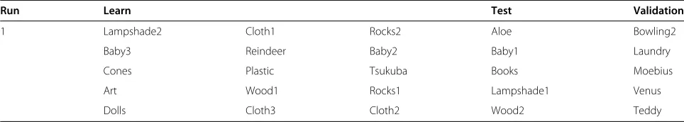
Even if no vigorous image analysis was used when choosing the images, both the learn- and test sets were carefully chosen by taking the following into consider-ation: (a) none of the sets contains known cases where the variational method is known to fail completely; (b) both very textured (e.g., Aloe and Cloth1) and less tex-tured cases (e.g., Plastic and Wood1) are included. Even though less textured cases are considerably more diffi-cult for stereo algorithms, these were included so that the parameters found by the DE algorithm would be more ‘generic’. In Appendix 1, Table 9, typical disparity values for each image are given, along with an example of the mean squared error for the calculated disparity maps. The reason for not including cases where the algorithm fails is that in these cases, the effect of the used image repre-sentation would be negligible and thus, would not convey useful information for our study. The variational methods (and any other method known to us) are known to fail with images that do not contain enough spatial features in order to approximate the disparity correctly. However, in [31] we propose a solution to this problem by using both spatial and temporal constraints.
K-fold cross-validation
Figure 3Stereo-images from the Middlebury database used in the quantitative experiments.(a)Aloe;(b)Art;(c)Baby1;(d)Baby2;(e) Baby3;(f)Books;(g)Bowling;(h)Cloth1;(i)Cloth2;(j)Cloth3;(k)Cones;(l)Dolls;(m)Lampshade1;(n)Lampshade2;(o)Laundry;(p)Moebius;(q) Plastic;(r)Reindeer;(s)Rocks1;(t)Rocks2;(u)Teddy;(v)Tsukuba;(w)Venus;(x)Wood1;(y)Wood2.
[32,33] to statistically test how well the obtained results are generalisable. In our case, due to the size of the data set, we use a 5-fold cross-correlation: the data set is bro-ken in five sets, each containing five images. Then, we run the DE and analyse the results five times using three of the sets for learning, one for validation, and one for testing. In each run the sets for learning, validation and testing will be different. Results are based on all of the five runs. Below, there is a list of sets for the first run (Table 4).
Information related to the image sets for all the different runs can be found in Appendix 1, Table 8.
Error metric
The error metric that we have used is the mean squared error (MSE), defined by:
MSE:= 1 SP
S
j=1
P
i=1
(di)j−(dgti)j 2
(31)
wheredis the calculated disparity map,dgtis the ground truth,Pis the number of pixels, andS is the number of images in the set (e.g., for a single imageS=1) for which the mean squared error is to be calculated for.
Table 4 Learn-, validation-, and test sets
Run Learn Test Validation
1 Lampshade2 Cloth1 Rocks2 Aloe Bowling2
Baby3 Reindeer Baby2 Baby1 Laundry
Cones Plastic Tsukuba Books Moebius
Art Wood1 Rocks1 Lampshade1 Venus
Results
In this section, we present the results, both quantity and visual quality-wise. First, the results are given by rank-ing how well each representation has done, both accu-racy and robustness-wise. Then, we study how combining different representations has affected the accuracy and the robustness of these combined representations. After this, we present the results for some real applications
visual quality-wise, since ground-truth is not available for these cases.
Ranking
Here, we rank each of the representation spaces in order to gain a better insight on the robustness and accuracy of each representation. By robustness and accuracy, we mean the following: (a) a representation is considered robust
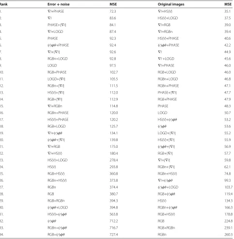
Table 5 Ranking for combined error+noise and original images
Rank Error+noise MSE Original images MSE
1. ∇I+PHASE 72.3 ∇I+HS(V) 35.1
2. ∇I 83.6 HS(V)+LOGD 37.5
3. PHASE+|∇I| 84.1 ∇I+RGB 39.0
4. ∇I+LOGD 87.4 ∇I+RGBn 39.4
5. PHASE 92.3 HS(V)+PHASE 40.6
6. (r)φθ+PHASE 92.4 (r)φθ+PHASE 42.2
7. ∇I+|∇I| 92.6 ∇I 44.9
8. RGBn+LOGD 92.8 ∇I+LOGD 45.6
9. LOGD 97.5 ∇I+PHASE 46.0
10. RGB+PHASE 102.7 RGB+LOGD 46.0
11. LOGD+|∇I| 105.5 RGBn+LOGD 46.8
12. RGBn+|∇I| 111.5 RGBn+PHASE 47.1
13. HS(V)+|∇I| 112.0 PHASE+|∇I| 47.7
14. RGB+|∇I| 112.9 RGB+PHASE 47.9
15. ∇I+RGBn 114.8 PHASE 48.3
16. RGBn+PHASE 120.0 LOGD 50.7
17. HS(V)+PHASE 120.2 HS(V)+(r)φθ 53.2
18. RGB+LOGD 125.7 (r)φθ 53.6
19. ∇I+(r)φθ 134.1 LOGD+|∇I| 55.2
20. (r)φθ+|∇I| 139.8 HS(V)+|∇I| 55.9
21. ∇I+RGB 175.0 (r)φθ+|∇I| 56.9
22. ∇I+HS(V) 180.4 RGB+|∇I| 57.7
23. HS(V)+LOGD 278.4 ∇I+|∇I| 59.8
24. HS(V) 293.8 RGBn+|∇I| 62.1
25. RGB+HS(V) 360.8 RGBn+HS(V) 74.8
26. RGBn+HS(V) 373.8 ∇I+(r)φθ 99.3
27. RGBn 374.4 (r)φθ+LOGD 103.7
28. RGB 380.7 RGB+(r)φθ 119.4
29. RGB+RGBn 394.3 HS(V) 134.3
30. (r)φθ+LOGD 394.8 RGBn+(r)φθ 166.3
31. HS(V)+(r)φθ 563.8 RGB+HS(V) 178.8
32. (r)φθ 712.2 RGB 224.8
33. RGBn+(r)φθ 716.7 RGB+RGBn 239.1
34. RGB+(r)φθ 727.4 RGBn 260.3
when results based on it are affected only slightly by noise or image errors; (b) a representation is considered accu-rate when results based on this gives good results using the original (i.e., noiseless) images. While this may not be the standard terminology, we find that using these terms makes it easier to explain the results. In Table 5, each of the representations is ranked with respect to (a) the
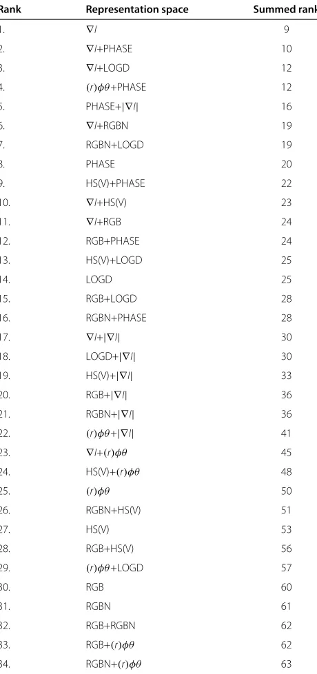
Table 6 Combined ranking
Rank Representation space Summed rank
1. ∇I 9
2. ∇I+PHASE 10
3. ∇I+LOGD 12
4. (r)φθ+PHASE 12
5. PHASE+|∇I| 16
6. ∇I+RGBN 19
7. RGBN+LOGD 19
8. PHASE 20
9. HS(V)+PHASE 22
10. ∇I+HS(V) 23
11. ∇I+RGB 24
12. RGB+PHASE 24
13. HS(V)+LOGD 25
14. LOGD 25
15. RGB+LOGD 28
16. RGBN+PHASE 28
17. ∇I+|∇I| 30
18. LOGD+|∇I| 30
19. HS(V)+|∇I| 33
20. RGB+|∇I| 36
21. RGBN+|∇I| 36
22. (r)φθ+|∇I| 41
23. ∇I+(r)φθ 45
24. HS(V)+(r)φθ 48
25. (r)φθ 50
26. RGBN+HS(V) 51
27. HS(V) 53
28. RGB+HS(V) 56
29. (r)φθ+LOGD 57
30. RGB 60
31. RGBN 61
32. RGB+RGBN 62
33. RGB+(r)φθ 62
34. RGBN+(r)φθ 63
The summed rank column is the sum of the rankings given in Table 5 for each representation. The ranking here is based on the summed rank (the lower, the better).
original images and (b) the combined illumination errors and noise types, while Table 6 combines the aforemen-tioned results into a single ranking. The MSE value in the tables is based on all the different runs (see Section 1). In the case of the combined error and noise (error+noise in the tables), the MSE value is calculated based on all the different illumination errors and noise types for the five different runs.
As can be observed from Table 5, the most robust rep-resentation was∇I+PHASE, while the second one was∇I without any combinations. Since both∇Iand PHASE rep-resent different physical quantities (gradient and phase of the image signal, as the names suggest), and both of these have been shown to be robust, it is not surprising that a combination of these was the most robust representation. In general, representations based on both∇Iand PHASE were amongst the most robust representations. On the other hand,∇I+LOGD was the most accurate representa-tion with the original images (i.e., without induced errors or noise). In general, representations based on ∇I have produced good results with the original images.
As can be observed from Table 6, the best combined
ranking was produced by ∇I alone. Also, it can be
noted that the first three are all based on ∇I. However, ∇I+PHASE is slightly more robust than∇Ialone, but not as accurate. This is clear from the figures presented in Section 1.
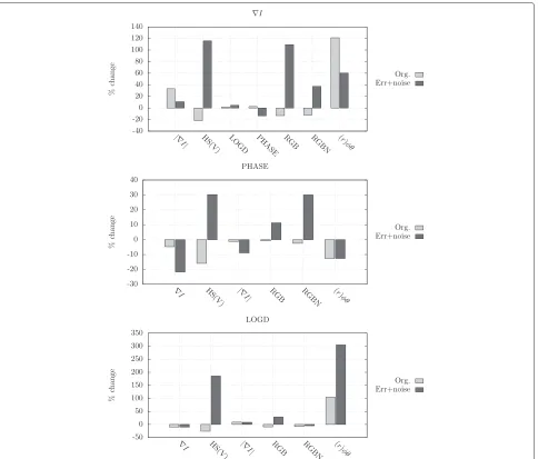
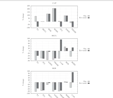
Improvement due to combined representation spaces In the following, we show how each of the basic represen-tations (1st column in Appendix 1, Table 7) has benefited, or worsened, by being combined with different represen-tations. In other words, we show, for example, how the error for∇Ichanges when combined with|∇I|, therefore, allowing us to deduce if∇Ibenefits from the combination. Results are given with respect to error, thus, a positive change in the error naturally means greater error and vice versa. Figure 4 displays the results for ∇I, PHASE, and LOGD, while Figure 5 gives the same for(r)φθ, HS(V) and RGB. We have left out results for RGBN on purpose, since this was the worst performer and the results, in general, were similar to those of RGB.
Figure 4Change in error due to combined representation.Results for∇I, PHASE, and LOGD. A positive value indicates an increase in error, while a negative value indicates a decrease in error.
Visual qualitative interpretation
Figures 6, 7, and 8 display results visually for the Cones, DRIVSCO, and GRASP cases, using the following image representations:∇I,∇I+PHASE,∇I+HS(V), PHASE, and RGB. A video of the results for DRIVSCO is available ath. These representations were chosen since (a)∇I was the overall ‘winner’ for the combined results (see Table 6); (b)∇I+PHASE was the most robust one; (c)∇I+HS(V) was the most accurate one; (d) PHASE is both robust and accurate, and (e) RGB is the ‘standard’ representation from typical cameras. The parameters used were the same in all the cases presented here and are those from the 1st run (out of five) for the 5-fold cross-validation. The rea-soning here is, confirmed by the results, that any robust
representation should be able to generate reasonable results for any of the parameters found in the cross-validation scheme.
As can be observed from Figure 6, the results are some-what similar for all the representations. However, as it can be observed, RGB has visually produced slightly worse results.
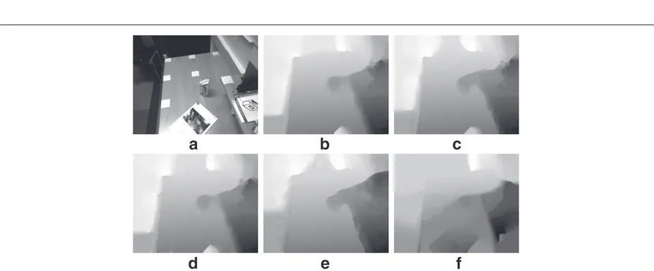
Figure 7 shows results for the DRIVSCOi sequence
Figure 5Change in error due to combined representation.Results for(r)φθ, HS(V), and RGB. A positive value indicates an increase in error, while a negative value indicates a decrease in error.
has produced very low quality results and, for example, scene interpretation based on these results would be very challenging if not impossible.
Figure 8 shows results for a robotic grasping scene. Both ∇Iand∇I+HS(V) have produced good results: the object of interest lying on the table is recognisable in the dis-parity map. ∇I+PHASE or PHASE alone has increased ‘leakage’ of disparity values between the object of interest and the shelf. On the other hand, PHASE representa-tion has produced the best results for the table, espe-cially for the lowest part. Again, RGB has produced low quality results.
Altogether, visual qualitative interpretation of the results using real image sequences is in line with the
quantitative analysis. Both ∇I and ∇I+PHASE produce good results even with real image sequences. However, the former produces slightly more accurate results while the latter representation is more robust.
Conclusions
Figure 6Cones.(a)Ground truth;(b)∇I;(c)∇I+PHASE;(d)∇I+HS(V);(e)PHASE;(f)RGB.
Figure 7DRIVSCO scene.(a)Left image;(b)∇I;(c)∇I+PHASE;(d)∇I+HS(V);(e)PHASE;(f)RGB.
10-fold (with noise and illumination errors) were found between the best and worst representation maps, which highlights the relevance of an appropriate input repre-sentation for low level estimations such as stereo. This accuracy enhancing and robustness to noise can be of critical importance in specific application scenarios with real uncontrolled scenes and not just well behaving test images (e.g., automatic navigation, advanced robotics, CGI). Amongst the tested combinations, the∇I represen-tation stood out as one of the most accurate and least affected by illumination errors or noise. By combining ∇Iwith PHASE, the joined representation space was the most robust one amongst the tested spaces. This finding was also confirmed by the qualitative experiments. Thus, we can say that the aforementioned representations com-plement each other. These results were also confirmed in a qualitative evaluation of natural scenes in uncontrolled scenarios.
There are some studies similar to ours, carried out in a smaller scale. However, the other studies typically pro-vide little information related to how the optimum (or near optimum) parameters of the algorithm are achieved, related to each representation space: in this study, we have used a well known, derivative free, stochastic algorithm called DE for the reasons given in the text. We argue that manually obtained parameters are subjected to a bias from the human operator and therefore, can be expected to confirm expected results. Three different sets of images were used for obtaining the parameters and testing each of the representations, in order to avoid over-fitting. The proposed methodology for estimating model parameters can be extended to many other computer vision algo-rithms. Therefore, our contribution should lead to more robust computer vision systems capable of working with real applications.
Future study
The weighting factors (b1andb2 in (1)) for each image
representation are applied equally to all of the ‘channels’.
Since some of the channels are more robust than others, like in the case of HSV for example, each channel should have its own weighting factor. Since this study allows us to cut down the number of useful representations, we pro-pose to study the best behaving ones in more detail with separate weighting factors where needed.
Appendix 1
Image representations and sets Typical disparity values
The following table displays minimum, maximum, mean, and standard deviation (STD) of ground-truth disparity for each of the used images. Also, in the same table we give the MSE (mean squared error), for each of the images, calculated using the parameters from the 1st run for the ∇Ibased image representation. The lowest numbers are the mean, standard deviation and MSE for the whole image set. The number on the lowest row in the table are the mean, standard deviation and MSE for the whole image set.
As it can be observed from Table 9, for some of the images the MSE is some what big. This does not come as a complete surprise since some of the images, such as Wood1, Wood2, Lampshade1, and Lampshade2 contain only few useful spatial features for approximating the dis-parity correctly. As future study, it would be interesting to divide the images into two categories (ones with sufficient spatial features and ones with only very few spatial fea-tures), and then search for the optimum parameters using the DE algorithm. Now, if there would be considerable improvement in either of the sets, then this would suggest that the parameters should be chosen based on previous image analysis step.
Endnotes
ahttp://www.jarnoralli.fi/.
bhttp://www.icsi.berkeley.edu/∼storn/code.html. chttp://vision.middlebury.edu/stereo/data/. dhttp://vision.middlebury.edu/stereo/data/.
Table 7 Tested image representation combinations
Term Term
None RGB RGBN |∇I| HS(V) (r)φθ Phase LOGD
None
RGB X X X X X X X
RGBN X X X X X X
∇I X X X X X X X X
HS(V) X X X X X
(r)φθ X X X X
Phase X X
Table 8 Learn-, validation-, and test sets
Run Learn Test Validation
1 Lampshade2 Cloth1 Rocks2 Aloe Bowling2
Baby3 Reindeer Baby2 Baby1 Laundry
Cones Plastic Tsukuba Books Moebius
Art Wood1 Rocks1 Lampshade1 Venus
Dolls Cloth3 Cloth2 Wood2 Teddy
2 Baby1 Cloth1 Teddy Art Rocks1
Aloe Wood1 Reindeer Baby2 Rocks2
Lampshade1 Laundry Bowling2 Cloth3 Cloth2
Dolls Wood2 Lampshade2 Plastic Books
Cones Baby3 Moebius Tsukuba Venus
3 Aloe Rocks1 Lampshade1 Baby1 Baby3
Dolls Venus Moebius Bowling2 Wood2
Laundry Tsukuba Rocks2 Lampshade2 Plastic
Cones Baby2 Books Reindeer Cloth2
Wood1 Art Cloth3 Teddy Cloth 1
4 Baby3 Cones Tsukuba Baby1 Books
Rocks2 Art Cloth3 Cloth2 Lampshade2
Laundry Dolls Reindeer Teddy Cloth1
Plastic Bowling2 Lampshade1 Venus Rocks1
Aloe Wood2 Baby2 Wood1 Moebius
5 Bowling2 Books Reindeer Baby2 Teddy
Tsukuba Cloth3 Rocks2 Cloth1 Baby3
Moebius Aloe Laundry Plastic Venus
Cones Wood1 Art Rocks1 Cloth2
Lampshade1 Dolls Lampshade2 Wood2 Baby1
Table 9 Typical disparity values for each image, and MSE for each image using parameters from the 1st run for∇I
image representation
Image Min Max Mean Std MSE
Aloe 14.33 70.33 24.13 9.34 43.7
Art 24.33 74.67 44.36 14.37 95.5
Baby1 8.33 45.33 27.79 10.66 24.6
Baby2 13.33 51.67 28.95 12.05 7.8
Baby3 15.67 51.00 42.15 6.93 11.7
Books 21.67 73.67 43.00 14.71 8.7
Bowling2 13.33 66.00 46.88 15.96 116.0
Cloth1 13.00 57.33 38.28 8.93 0.6
Cloth2 14.00 76.00 53.24 12.37 30.6
Cloth3 15.00 55.33 36.28 11.31 5.1
Cones 5.50 55.00 33.54 11.58 8.7
Dolls 3.00 73.67 45.85 14.09 4.2
Lampshade1 14.00 64.67 35.87 15.90 78.2
Table 9 Typical disparity values for each image, and MSE for each image using parameters from the 1st run for∇I
image representation(continued)
Laundry 11.67 77.33 40.29 12.95 27.3
Moebius 21.33 72.67 37.19 11.20 12.7
Plastic 7.67 65.33 45.27 13.36 15.4
Reindeer 3.67 67.00 41.54 15.01 112.8
Rocks1 19.33 56.67 37.53 9.50 1.7
Rocks2 23.33 56.00 38.57 7.00 1.3
Teddy 12.50 52.75 27.38 9.02 8.8
Tsukuba 5.00 14.00 6.79 2.67 2.1
Venus 3.00 19.75 8.89 4.09 1.0
Wood1 21.67 71.67 40.83 12.71 102.5
Wood2 14.33 72.33 48.89 15.46 126.6
37.08 15.82 36.9
ehttp://vision.middlebury.edu/stereo/data/. fhttp://www.pspc.dibe.unige.it/∼drivsco/. ghttp://www.csc.kth.se/grasp/.
hhttp://www.jarnoralli.fi/.
ihttp://www.jarnoralli.fi/joomla/publications/
representation-space.
Additional file
Additional file 1: DRIVSCO sequence disparity results.Disparity calculation results for the DRIVSCO sequence using different image representations.
Competing interests
The authors declare that they have no competing interests.
Acknowledgements
We thank Dr. Javier S´anchez and Dr. Luis ´Alvarez from the University of Las Palmas de Gran Canaria, and Dr. Stefan Roth from the technical University of Darmstadt for helping us out getting started with the variational methods. Further, we would like to thank Dr. Andr´es Bruhn for our fruitful conversations during the DRIVSCO workshop 2009. Also, we would like to thank the PDC Center for High Performance Computing of Royal Institute of Technology (KTH, Sweden) for letting us use their clusters. This work was supported by the EU research project TOMSY (FP7-270436), the Spanish Grants DINAM-VISION (DPI2007-61683) and RECVIS (TIN2008-06893-C03-02), Andalusia’s regional projects (P06-TIC-5060 and TIC-3873) and Granada Excellence Network of Innovation Laboratories’ project PYR-2010-19.
Received: 16 September 2011 Accepted: 13 November 2012 Published: 10 December 2012
References
1. BKP Horn, BG Schunck, Determining optical flow. Artif. Intell.17, 185–203 (1981)
2. Y Huang, K Young, Binocular image sequence analysis: integration of stereo disparity and optic flow for improved obstacle detection and tracking. EURASIP J. Adv. Signal Process.2008, 10 (2008)
3. M Bj ¨orkman, D Kragic, inProceedings of the British Machine Vision Conference. Active 3D segmentation through fixation of previously unseen objects (BMVA Press, 2010), pp. pp. 119.1–119.11. doi:10.5244/C.24.119 4. Y Mileva, A Bruhn, J Weickert, inDAGM07- Volume LNCS, vol. 4713.
Illumination-robust variational optical flow with photometric invariants (Heidelberg, Germany, 2007), pp. 152–162
5. C W ¨ohler, P d’Angelo, Stereo image analysis of non-lambertian surfaces. Int. J. Comput. Vision.81(2), 172–190 (2009)
6. B Maxwell, R Friedhoff, C Smith, inin IEEE Conference on Computer Vision and Pattern Recognition (CVPR 2008). A bi-illuminant dichromatic reflection model for understanding images (Anchorage, Alaska, USA, 2008), pp. 1–8 7. S Shafer, Using color to separate reflection components. Tech. rep (1984).
[TR 136, Computer Science Department, University of Rochester] 8. DG Lowe, Distinctive image features from scale-invariant keypoints. Int. J.
Comput. Vision.60, 91–110 (2004)
9. H Bay, A Ess, T Tuytelaars, LV Gool, Speeded-up robust features (SURF). Comput. Vis. Image Underst.110, 346–359 (2008)
10. A Bruhn, Variational optic flow computation: accurate modelling and efficient numerics.PhD thesis, Saarland University, Saarbr ¨ucken, Germany (2006)
11. T Brox, From pixels to regions: partial differential equations in image analysis.PhD thesis, Saarland University, Saarbr ¨ucken, Germany (2005) 12. A Bruhn, J Weickert, T Kohlberger, C Schn ¨orr, A multigrid platform for real-time motion computation with discontinuity-preserving variational methods. Int. J. Comput. Vision.70(3), 257–277 (2006)
13. N Slesareva, A Bruhn, J Weickert, inDAGM05- Volume LNCS 3663. Optic flow goes stereo: a variational method for estimating discontinuity-preserving dense disparity maps (Vienna, Austria, 2005), pp. 33–40
14. T Brox, A Bruhn, N Papenberg, J Weickert, inECCV04-Volume LNCS 3024. High accuracy optical flow estimation based on a theory for warping (Prague, Czech Republic, 2004), pp. 25–36
15. M Black, P Anandan, inProc. Computer Vision and Pattern Recognition. Robust dynamic motion estimation over time (Maui, Hawaii, USA, 1991), pp. 296–302
16. J Weickert, C Schn ¨orr, A theoretical framework for convex regularizers in PDE-based computation of image motion. Int. J. Comput. Vision.45(3), 245–264 (2001)
17. H Nagel, W Enkelmann, An investigation of smoothness constraints for the estimation of displacement vector fields from image sequences. PAMI.8(5), 565–593 (1986)
18. L Alvarez, J Weickert, J S´anchez, Reliable estimation of dense optical flow fields with large displacements. Int. J. Comput. Vision.39, 41–56 (2000)
19. H Zimmer, A Bruhn, J Weickert, L Valgaerts, A Salgado, B Rosenhahn, H Seidel, inEMMCVPR , vol. 5681 of Lecture Notes in Computer Science. Complementary optic flow (Bonn, Germany, 2009), pp. 207–220 20. A Blake, A Zisserman,Visual Reconstruction. (The MIT Press, Cambridge,
Massachusetts London, England, 1987)
21. U Trottenberg, C Oosterlee, A Sch ¨uller,Multigrid, (Academic Press, A Harcourt Science and Technology Company Harcourt Place. 32 Jamestown Road, London NW1 7BY UK, 2001)
23. R Storn, K Price, Differential evolution—a simple, efficient heuristic for global optimization over continuous spaces. J. Global Optimiz.11(4), 341–359 (1997)
24. VP Plagianakos, MN Vrahatis, Parallel evolutionary training algorithms for hardware-friendly neural networks. Nat. Comput.1, 307–322 (2002) 25. DK Tasoulis, N Pavlidis, VP Plagianakos, MN Vrahatis, inIn IEEE Congress on
Evolutionary Computation (CEC). Parallel differential evolution, (Portland, OR, USA, 2004), pp. 1–6
26. MG Epitropakis, VP Plagianakos, MN Vrahatis, Hardware-friendly higher-order neural network training using distributed evolutionary algorithms. Appl. Soft Comput.10, 398–408 (2010)
27. D Hubel, T Wiesel, Anatomical demonstration of columns in the monkey striate cortex. Nature.221, 747–750 (1969)
28. D Fleet, A Jepson, Stability of phase information. IEEE Trans. Pattern Anal. Mach. Intell.15(12), 1253–1268 (1993)
29. D Fleet, A Jepson, Phase-based disparity measurement. Comput. Vision Graphics Image Process.53(2), 198–210 (1991)
30. S Sabatini, G Gastaldi, F Solari, K Pauwels, MV Hulle, Jx D´ıaz, J Ros, N Pugeault, N Kr ¨uger, A compact harmonic code for early vision based on anisotropic frequency channels. Comput. Vis. Image Underst.114, 681–699 (2010)
31. J Ralli, J D´ıaz, E Ros, Spatial and temporal constraints in variational correspondence methods. Mach. Vision Appl, 1–13 (2011)
32. PA Devijver, J Kittler,Pattern Recognition: a Statistical Approach. (Prentice Hall, 1982). ISBN 13: 9780136542360, ISBN 10: 0136542360
33. R Kohavi, inProceedings of the 14th International Joint Conference on Artificial Intelligence- Volume 2. A study of cross-validation and bootstrap for accuracy estimation and model selection, (Morgan Kaufmann, Montreal, Quebec, Canada, 1995), pp. 1137–1143
doi:10.1186/1687-6180-2012-254
Cite this article as:Ralliet al.:Experimental study of image representation spaces in variational disparity calculation.EURASIP Journal on Advances in
Signal Processing20122012:254.
Submit your manuscript to a
journal and benefi t from:
7 Convenient online submission 7 Rigorous peer review
7 Immediate publication on acceptance 7 Open access: articles freely available online 7 High visibility within the fi eld
7 Retaining the copyright to your article