An Optofluidic Ring Resonator Platform for Rapid and Robust Sensing

(1)

for the Degree of Doctor of Philosophy

CALIFORNIA INSTITUTE OF TECHNOLOGY Pasadena, California

2017

(2)

c 2017

(3)

teractions, drug screening, and point-of-care diagnostics. They are sensitive to minute changes in the refractive index of the surrounding medium, which enables them to detect and quantify sub-femtomolar concentrations of target molecules. This thesis investigates the advantages of an optofluidic ring resonator platform that employs a differential measurement scheme for reducing environmental noise due to temperature and pressure fluctuations. Through simulations and exper-iments, I determine the sensitivity of the platform to changes in the target analyte concentration and to environmental noise, and demonstrate the benefits of employing a second, reference, ring resonator.

(4)

Published Content and

Contributions

D. Kim, P. Popescu, M. Harfouche, J. Sendowski, M.-E. Dimotsantou, R. C. Flagan, and A. Yariv, “On-chip integrated differential optical microring refractive index sensing platform based on a lam-inar flow scheme,”Opt. Lett., vol. 40, pp. 4106-4109, Sep 2015. doi:10.1364/OL.40.004106.

P. Popescu contributed by designing and fabricating the microfluidic chips, participated in the experimental setup, the preparation of the reagents and the collection and interpretation of data.

D. Kim, P. Popescu, M. Harfouche, J. Sendowski, M.-E. Dimotsantou, R. Flagan, and A. Yariv, “On-chip integrated differential optical microring biosensing platform based on a dual laminar flow

(5)

(6)

Acknowledgments

My graduate career at Caltech was a complex and formative journey, and I was fortunate to have the guidance and support of a number of people who have been instrumental in the successful completion of my project and degree.

First and foremost I want to thank my advisor, Prof. Richard Flagan, for his unwavering support and excellent mentorship. He was always available when I needed his input, and always eager to discuss and brainstorm ideas related to the project. He trusted me to take the project in the directions that I envisioned, but also guided me along the way. Under his supervision I have grown tremendously as a scientist and independent researcher. It’s not an overstatement to say that I could not have asked for a better advisor and mentor.

Prof. Amnon Yariv, whom I consider my unofficial co-advisor, has been a great source of deep insights into optics, and has provided invaluable advice during my meetings with him. In addition, I have enjoyed the discussions during the group meeting lunch on many diverse topics including science, literature and linguistics.

Prof. Keith Schwab has been a mentor throughout my graduate career. I am very grateful for his support during difficult times in my career, which was crucial to my continued success.

I am grateful for the input and advice of Prof. Andrei Faraon during the committee meetings in the last years of my graduate life.

I would not have had the opportunity of working on this project without Prof. Scott Fraser’s guidance. In addition, over the first few years of my graduate life, he has put me in contact with experts in the field, and provided many resources from his lab that helped me further my experiments. I would also like to thank the Graduate Dean’s Office, in particular Felicia Hunt, Natalie Gilmore, Doug Reese, and Joe Shepherd for their support and their help in navigating the intricacies of graduate life.

(7)

My life at Caltech would not have been the same without an amazing group of friends. Thank you to Ron Appel and Becky Calinsky for many fun times and pleasantries. The elbow house and its residents, Kevin Engel, Evan O’Connor, Milivoje Lukic, and Dan Betea, hold a special place in my heart. We have shared many fond memories and exciting adventures. Itamar Yaakov has been a caring and kind friend. I could always count on Vaclav Cvicek and Diana Negoescu for help and advice. Thank you to Mihai Florian for his encouraging words and generosity. I dearly cherish the friendship of Laura Book, Esfandiar Alizadeh, and Hesham Azizgolshani, who are very warm and big-hearted. Many thanks to Mhair Orchanian, Tim Morton, Vera Gluscevic, Tomasz Tyranowski, Bao Ha, Andrew Richards, Kari Hodge and Henry Kozachkov for the wonderful memories we have made during these years. I miss the orienteering trips I took with Malena and Augustin. Thank you Ayfer, Francisco and Kaloyan for not letting time and distance keep us apart.

I am deeply grateful to my parents, Sanda and Bob, for their unconditional love and selflessness, for always believing in me, for wanting what’s best for me, and for making many sacrifices to see me succeed in my endeavors.

(8)

List of Figures

2.1 Water absorption coefficient at various wavelengths of light. The data from Segelstein [1] covers a wider range, but the data from Kedenburget al. [2] is denser in the range of interest. The two sets of data agree fairly well, giving a coefficient of absorption about two orders of magnitude larger at 1550 nm than at 1064 nm. . . 12

2.2 a) Mode profile of ring resonator for TE mode in water. b) Mode profile for TM mode in water. . . 14

2.3 Mode profile along a vertical section through the center of resonator. The different colors indicate the different media through which the mode propagates. By fitting a decaying exponential to the tail of the evanescent field inside water, we obtain a decay constant of 160 nm. . . 16

2.4 a) The evanescent tail of the mode interacts with a bulk solution b) The evanescent tail of the mode interacts with a surface organic layer. . . 17

2.5 RecordedQ-factors of two fabricated rings coupled to the same waveguide. . . 17

2.6 a) SEM picture of the ring resonator geometry b) SEM picture of the coupling region between the bus waveguide and the ring resonator. Pictures courtesy of Dongwan Kim. 18

2.7 a) Change in resonant frequency as a function of salt concentration, for a ring resonator with waveguide height ofh= 250 nm and ring width ofw= 1µm. . . 19

2.8 Change in resonant frequency as a function of the thickness of the organic layer. . . . 20

2.9 Equilibration of concentration and temperature inside the channel . . . 24

2.10 a) Resonant frequency as a function of waveguide height b) Resonant frequency as a function of ring width.. . . 25

2.11 a) Sensitivity to bulk index of refraction changes as a function of ring height b) Sensi-tivity to bulk index of refraction changes as a function of ring width.. . . 25

2.12 a) Sensitivity to surface sensing as a function of ring height b) Sensitivity to surface sensing of as a function of ring width. . . 26

2.13 a) Temperature sensitivity as a function of waveguide height b) Temperature sensitivity as a function of ring width. . . 26

(11)

2.18 Temperature calibrations in water. The first subplot shows the response of the sensing and reference resonators. The reference resonator response has been shifted upwards by 2 GHz for ease of visualization. The second subplot shows the differential signal, on a scale 6 times smaller. . . 30

2.19 Temperature calibrations in water. The first subplot shows the stage temperature cycles. The second subplot shows the response of the sensing and reference resonators. The reference resonator response has been shifted upwards by 2 GHz. The third subplot shows the differential signal. . . 31

2.20 Resonator response to cycles of 40 mM NaCl in a temperature varying environment. Temperature shifts affect the individual resonator responses, but not the differential signal. . . 32

2.21 Resonator response to changes in inlet pressure in increments of ∆p=14 kPa (2 psi). . 33

2.22 a) Dual-flow platform. b) Covered reference ring platform. . . 34

2.23 a) Allan deviation in dual flow platform. b) Allan deviation in covered platform. . . . 34

2.24 a) Allan deviation in air. . . 35

3.1 Initial setup that includes syringe pumps and a three-way solenoid valve to control the flow to the resonator chip. Two syringe pumps containing the buffer (blue) and the analyte of interest (orange) are connected to the three-way solenoid valve, which is computer-controlled. We can switch the flow from either of the first two syringe pumps and direct it to the sensing resonator. A third syringe pump with buffer (blue) is continuously flowing to the reference resonator. . . 39

(12)

3.3 A schematic diagram of the fluidic control of the solutions delivered to the PDMS chip. Two regulators control the pressures for the control and flow layer. The control layer tubing is connected to a solenoid manifold that turns the valve for each control channel

on or off. . . 41

3.4 a) Closed control valves for three out of the four inlets. b) Backflow into adjacent channels. . . 42

3.5 Schematic of the two-layer microfluidic chip. The control layer (in orange), is situated on top of the flow layer (in blue). The four inlets of the flow layer are labeled from 1-4. We can introduce a solution at either one, and either allow or restrict the flow using the corresponding control layer channel and associated valve. . . 43

3.6 A typical sensing experiment involves three steps: setting up the baseline, introducing the analyte and re-establishing to the baseline. . . 44

3.7 On-chip valve platform response to a concentration of 160 mM of NaCl. . . 45

3.8 Differential resonator response as inlets with buffer switch from inlets 1 and 4 to inlets 2 and 3. . . 46

3.9 Differential resonator response as inlets with buffer switch from inlets 1 and 4 to inlets 2 and 4. . . 47

3.10 Two chip platform . . . 48

3.11 Response time in two-chip platform. . . 48

3.12 Switching transients in the two-chip platform.. . . 49

3.13 Experimental data (in red) for the two-chip platform response to concentrations of salt of 80mM and 160mM (the larger response is for the larger concentration). Theoretical curves based on the Taylor dispersion model (in blue) match the experimental data very well. . . 52

3.14 Experimental data (in red) for the solenoid setup response to a concentration of salt. The theoretical fit based on the Taylor dispersion model coupled to a continuous stirred tank reactor (in blue) matches very well the experimental data.. . . 53

4.1 Silanization step in which an aminosilane first forms covalent siloxane bonds to the surface, then crosslinks to adjacent aminosilane molecules . . . 56

4.2 a) AFM measurement of piranha cleaned chip. b) Detailed scan of the piranha cleaned chip. . . 58

(13)

4.8 Fluorescence image showing the attachment of FITC to APTMS. In the left figure we show a blank wafer to which FITC has been added. The intensity is very low, indicating that FITC has not attached to the substrate in the absence of a linker layer. In the center image, APTMS has been added to the nitride, but again there is no fluorescence. In the left image, FITC has been added to the APTMS-coated nitride, resulting in a high intensity fluorescence signal. This indicates that FITC only binds to the substrate in the presence of APTMS. . . 64

4.9 Chemistry of coumarin addition and photouncaging. . . 65

4.10 The left image shows the sample with coumarin attached. The right image shows that coumarin has been selectively removed from the resonator surface . . . 65

4.11 The top row shows the sample after coumarin was deposited. The left panel shows the fluorescence under settings for coumarin detection (left) and under settings for FITC detection (right). The bottom row shows the same area on the same sample after FITC has been deposited. . . 66

5.1 Schematic of the three mechanisms involved in delivering the analyte to the sensor surface: convection, diffusion, and reaction. . . 70

5.2 a) Development of the concentration boundary layer if the entire bottom surface of the channel is reactive. b) Development of the concentration boundary layer if only the resonator surface is reactive. . . 71

5.3 Schematic geometry of channel with two chevrons. . . 75

5.4 (a) Streamlines closes to the top of the channel are deflected most by the groove. (b) Streamlines in the middle of the channel are deflected. (c) Streamlines close to the bottom of the channel are not deflected. . . 77

5.5 Effect of one groove on the flux along the midline of the channel. . . 78

(14)

5.7 a) Flux enhancement factor for a groove of widtha= 60µm for four different groove depths as a function on inlet velocity. b) Flux enhancement factor for a groove of width

a= 120µm for four different groove depths as a function on inlet velocity.) . . . 80

5.8 Flux enhancement factor as a function of groove width a for four different groove depths. The left plot is for a channel height H = 20µm, and the right plot for a channel height ofH = 40µm . . . 80

5.9 Bezier curves for defining new chevron shapes. . . 81

5.10 Improvement as function of depth of groove . . . 82

5.11 Schematic of two-groove herringbone, showing the overall footprint of the structure . 83

5.12 Flux improvement for a two-groove geometry withd= 20µm,d= 40µm, andd= 80µm. 84

5.13 Flux improvement for a two-groove geometry with Bezier shape. . . 84

5.14 Flux improvement for a two groove geometry compared to a one groove geometry composed of only the last groove.. . . 85

5.15 Flux improvement for a three-groove geometry as we vary the last groove width. . . . 86

5.16 Four-groove geometry flux as a function of groove width and spacing. . . 87

5.17 Influence of shape of herringbone in four-groove geometry.. . . 88

5.18 Time evolution of the flux and surface concentration in a simple channel withH = 40µm. 89

5.19 Steady state flux if only the resonator is passivated inH = 40µm. . . 89

6.1 A dual laminar flow platform with herringbone grooves for enhanced mass transport to the sensors. . . 94

(15)

2.2 Indexes of refraction and thermo-optic coefficients for the materials employed. . . 22

2.3 Calculated values of the confinement factors for three upper cladding media and the resulting temperature sensitivities. . . 22

2.4 Materials used for covering the reference resonator.. . . 23

3.1 Various geometries of the fluidic channels and flow characteristics employed by different groups. . . 39

3.2 Flow characteristics in the on-chip switching platform. . . 45

4.1 Percentage atomic concentration for the detected elements in three sample with differ-ent chemistries. . . 60

4.2 Thickness of silane layers for four different deposition conditions for a solution of 1 mM APTMS. . . 62

5.1 Boundary conditions for the steady state laminar flow equations. . . 74

5.2 Convection-diffusion boundary conditions . . . 75

(16)

Chapter 1

Introduction

Biosensors are versatile tools used for medical applications in clinical diagnostics, drug screening, and pathogen detection, as well as for fundamental science in studies of binding kinetics and epitope mapping. Affinity biosensors rely on the specific interaction between a biorecognition element such as an enzyme, antigen, or nucleic acid, and the analyte of interest. A signal transduction mechanism converts the biomolecular interaction into a readable and quantifiable signal. Depending on the nature of the transduction mechanism, most biosensors can be categorized as mechanical, electrical, or optical. This thesis presents the development of an optical ring resonator biosensor platform, an emergent optical biosensor technology, and explores designs and protocols for enabling it to simultaneously achieve low detection limits, fast assay times, and parallel sensing, a highly desirable combination of qualities for a biosensor. First we give a brief overview of biosensor platforms in general, and their biological applications, touching upon some of the advantages and drawbacks of each platform. We focus on optical biosensors, with emphasis on whispering gallery mode resonators. Detailed reviews on optical biosensors and microring resonators can be found in [1,2, 3,4,5].

1.1

Overview of biosensing technologies

(17)

order to obtain an accurate disease diagnosis [6]. Moreover, biosensors can be employed in single cell analysis by detecting cytosolic-level concentrations of cytokines from single cell lysis or cell se-cretion in microfluidic chambers. Arlett et al. give an overview of different biosensor technologies and their detection capabilities, and suggest the benchmark detection to be a concentration increase of 40 fM min−1_{, which is the secretion rate of tumor necrosis factor-α}_{(TNF-α), a cancer biomarker,}

by monomyelectic cells [7]. The limit for biosensing is, ultimately, single molecule detection; this sensitivity would give insight into fundamental binding processes and kinetics, well beyond those possible with ensemble averages.

In addition to classifying biosensors in terms of their signal transduction scheme, they may be divided into sensors in which the target analyte or the receptor biorecognition element is either labeled or unlabeled. The label can be either a fluorescent or radioactive tag. Labeling the analyte may alter the interaction affinity and binding kinetics; it is also a time-consuming and laborious procedure. For radioactive labels, there is an added cost that arises from the generation of hazardous waste and handling of radioactive substances. Therefore, label-free detection schemes are preferred over labeled ones.

This thesis focuses on a label-free detection scheme based on integrated optical resonators. In the discussion that follows, we will first give an overview of mechanical and electrical biosensors, and devote the next section to optical resonators.

(18)

are part of a larger class of sensors based on surface acoustic waves (SAW). Both MCs and QCMs have detection limits in the picomolar range and have been commercialized.

Electrical biosensors include modified field effect transistors (FETs) that respond to biomolecular interactions that alter the electrical properties of a semiconductor nanowire that connects the source electrode (S) and the drain electrode (D) of the FET. A voltage applied to a gate electrode (G) influences the conductivity of the channel between the source and the drain. For biosensing, the source and drain electrodes are connected using either a semiconductor nanowire (NW) or carbon nanotubes (CNTs) functionalized with a biorecognition element. When charged molecules of the analyte bind to either the NW or to the CNTs, the resulting change in the conductivity of the channel provides a signal from which one can infer the concentration of the target molecule. A drawback of bionsensor FETs is the small size of the sensor, which results in a very small mass transport, and, thus, a lengthy assay time, sometimes on the order of days [7]. Moreover, FET-based biosensors are also difficult to integrate with ionic solutions and buffers, due to Debye screening, such as that which occurs when charged positive ions screen the negatively charged DNA strands [8].

1.1.1

Optical biosensors: Fluorescence and Refractive Index Detection

(19)

light as it undergoes total internal reflection at the interface with the metal. Resonance that occurs when the momentum of the incident light matches that of the plasmon wave, generates a surface wave. At resonance, a light beam reflected from the metal surface exhibits a minimum in intensity. When the refractive index of the exit dielectric medium changes due to binding of analyte to the metal, the momentum of the surface wave also changes, leading to a shift in the angle of incidence of the incoming light at which the light-beam momentum matches that of the plasmon wave. By monitoring the incident angle at resonance, the concentration of bound analyte to the metal surface can be inferred.

A novel optical biosensor, the photonic crystal, relies on a defect inside a periodic dielectric nanostructure that allows a single resonant frequency to propagate inside the structure. When the refractive index around the defect changes to the presence of the analyte, the resonant frequency changes as well, indicating the amount of bound analyte. Photonic crystals are usually achieved in either 1D or 2D.

Other high sensitivity refractive index sensors also rely on detecting shifts in resonances within interferometers, waveguides, optical fibers, and other devices.

Lastly, microcavity whispering gallery mode (WGM) resonators exploit the resonance condition established when a beam of light is confined by total internal reflection inside a circular structure. The evanescent field of the optical mode samples the index of refraction of the surrounding medium. When an analyte enters the evanescent field, it changes the propagation speed of the light, influencing the resonance condition which is detected as a minimum in the frequency transmission spectrum. This thesis focuses on one type of whispering gallery mode resonator.

1.1.2

Microcavity whispering gallery mode resonators

(20)

res-onators are thin capillaries, and they are easy to fabricate and compatible with fluid delivery. Mi-crosphere resonators are also easy to fabricate, and achieve very high sensitivities, but they are hard to integrate into multiplexed platforms. Microtoroids can be fabricated and integrated easily, but they are delicate, and the light coupling between the fiber and the sensor is not robust. Planar ring and disk resonators offer the most robust and reproducible fabrication, compatible with silicon processing technology, are easily multiplexed, and can be easily integrated with a fluidic delivery system. In this work we will use planar ring resonators, since they are the most promising among WGM sensors.

1.2

Applications

A major application of biosensors is for the medical industry, in performing assays for clinical diagno-sis and drug engineering. Moreover, they have applications in protein analydiagno-sis, DNA hybridization assays, and detection of viruses, bacteria, and cells. In terms of fundamental research, they are employed in characterizing biomolecular interactions and extracting real-time binding kinetics infor-mation. Other areas include environmental monitoring and food testing for toxins and pathogens.

Protein analysis is based on the high affinity binding of antibodies to antigens, or of engineered aptamers to target molecules. The latter technique allows for engineering receptors for an unlimited number of target analytes by selectively and predictably folding short DNA sequences. The synthesis of aptamers is very reproducible, and they are less prone to denaturation than proteins; this makes them excellent tools in biorecognition [10]. One major application of protein analysis is for cancer diagnosis through the detection of cancer and inflammation biomarkers in serum. For example, two breast cancer biomarkers, CA15-3 and HER2, have been detected in blood serum by different groups [11,12]. Washburnet al. detected a colorectal cancer biomarker, carcinoembryonic antigen (CEA) [13]. It was followed by multiplexed detection of five protein biomarkers, among which three cancer biomarkers: tumor necrosis factor-α(TNF-α), prostate specific antigen (PSA), and CEA, as well as two inflammation markers: α-fetoprotein (AFP) and interleukin-8 (IL-8), paving the way for fingerprint biomarker assays [14]. Recently, they detected up to eight cancer biomarkers simultaneously [15]. Moreover, detection of pathogen biomarkers against the Ebola virus, Marburg virus, and dengue virus have been reported [16]. Another set of protein detection assays are aimed at studying kinetic binding rates, such as the streptavidin-biotin interaction [17]

(21)

detected single Influenza A virus of radius 50 nm from a concentration of 10 fM [26]. Sloanet al. investigated the interaction between proteins and the cell membrane using phospholipid bilayer nanodiscs [27]

1.3

Thesis Structure

(22)

and show how geometrical parameters influence its effect on the response time. Lastly, Chapter 6 offers possible future directions, and design improvements.

Bibliography

[1] X. Fan, I. M. White, S. I. Shopova, H. Zhu, J. D. Suter, and Y. Sun, “Sensitive optical biosensors for unlabeled targets: A review,”Analytica Chimica Acta, vol. 620, no. 12, pp. 8 – 26, 2008.

[2] H. Zhu, J. D. Suter, and X. Fan, Optical Guided-wave Chemical and Biosensors II, ch. Label-Free Optical Ring Resonator Bio/Chemical Sensors, pp. 259–279. Springer Berlin Heidelberg, 2010.

[3] J. T. Kindt and R. C. Bailey, “Biomolecular analysis with microring resonators: applications in multiplexed diagnostics and interaction screening,” Current Opinion in Chemical Biology, vol. 17, no. 5, pp. 818 – 826, 2013.

[4] Y. Sun and X. Fan, “Optical ring resonators for biochemical and chemical sensing,”Analytical and Bioanalytical Chemistry, vol. 399, no. 1, pp. 205–211, 2011.

[5] A. P. F. Turner, “Biosensors–sense and sensitivity,” Science, vol. 290, no. 5495, pp. 1315–1317, 2000.

[6] R. Malhotra, V. Patel, J. P. Vaqu, J. S. Gutkind, and J. F. Rusling, “Ultrasensitive electro-chemical immunosensor for oral cancer biomarker IL-6 using carbon nanotube forest electrodes and multilabel amplification,”Analytical Chemistry, vol. 82, no. 8, pp. 3118–3123, 2010.

[7] J. L. Arlett, E. B. Myers, and M. L. Roukes, “Comparative advantages of mechanical biosen-sors,”Nature Nanotechnology, vol. 6, pp. 203 – 215, 2011.

[8] E. Stern, R. Wagner, F. J. Sigworth, R. Breaker, T. M. Fahmy, and M. A. Reed, “Importance of the Debye screening length on nanowire field effect transistor sensors,”Nano Letters, vol. 7, no. 11, pp. 3405–3409, 2007.

[9] B. Liedberg, C. Nylander, and I. Lunstrm, “Surface plasmon resonance for gas detection and biosensing,”Sensors and Actuators, vol. 4, pp. 299 – 304, 1983.

[10] W. Zhou, P.-J. Jimmy Huang, J. Ding, and J. Liu, “Aptamer-based biosensors for biomedical diagnostics,”Analyst, vol. 139, pp. 2627–2640, 2014.

[11] H. Zhu, P. S. Dale, C. W. Caldwell, and X. Fan, “Rapid and label-free detection of breast cancer biomarker CA15-3 in clinical human serum samples with optofluidic ring resonator sensors,”

(23)

resonators,”Analytical Chemistry, vol. 82, no. 1, pp. 69–72, 2010.

[15] A. L. Washburn, W. W. Shia, K. A. Lenkeit, S.-H. Lee, and R. C. Bailey, “Multiplexed cancer biomarker detection using chip-integrated silicon photonic sensor arrays,”Analyst, pp. –, 2016.

[16] I. A. Estrada, R. W. Burlingame, A. P. Wang, K. Chawla, T. Grove, J. Wang, S. O. Southern, M. Iqbal, L. C. Gunn, and M. A. Gleeson, “Multiplex detection of pathogen biomarkers in human blood, serum, and saliva using silicon photonic microring resonators,” Proc. SPIE, vol. 9490, pp. 94900E–94900E–14, 2015.

[17] C. E. Soteropulos, H. K. Hunt, and A. M. Armani, “Determination of binding kinetics using whispering gallery mode microcavities,”Applied Physics Letters, vol. 99, no. 10, 2011.

[18] J. D. Suter, I. M. White, H. Zhu, H. Shi, C. W. Caldwell, and X. Fan, “Label-free quantitative DNA detection using the liquid core optical ring resonator,” Biosensors and Bioelectronics, vol. 23, no. 7, pp. 1003 – 1009, 2008.

[19] J. D. Suter, D. J. Howard, C. W. Caldwell, H. Shi, and X. Fan, “Label-free DNA methylation analysis using the optofluidic ring resonator sensor,”Proc. SPIE, vol. 7322, pp. 732208–732208– 8, 2009.

[20] F. Vollmer, S. Arnold, D. Braun, I. Teraoka, and A. Libchaber, “Multiplexed DNA quantifi-cation by spectroscopic shift of two microsphere cavities,” Biophysical Journal, vol. 85, no. 3, pp. 1974 – 1979, 2003.

[21] A. Ramachandran, S. Wang, J. Clarke, S. Ja, D. Goad, L. Wald, E. Flood, E. Knobbe, J. Hryniewicz, S. Chu, D. Gill, W. Chen, O. King, and B. Little, “A universal biosensing platform based on optical micro-ring resonators,”Biosensors and Bioelectronics, vol. 23, no. 7, pp. 939 – 944, 2008.

(24)

photonic microring resonator arrays,” Analytical Chemistry, vol. 83, no. 17, pp. 6827–6833, 2011.

[23] A. Qavi and R. Bailey, “Multiplexed detection and label-free quantitation of microRNAs using arrays of silicon photonic microring resonators,” Angewandte Chemie International Edition, vol. 49, no. 27, pp. 4608–4611, 2010.

[24] S. Arnold, R. Ramjit, D. Keng, V. Kolchenko, and I. Teraoka, “Microparticle photophysics illuminates viral bio-sensing,”Faraday Discuss., vol. 137, pp. 65–83, 2008.

[25] H. Zhu, I. M. White, J. D. Suter, M. Zourob, and X. Fan, “Opto-fluidic micro-ring resonator for sensitive label-free viral detection,”Analyst, vol. 133, pp. 356–360, 2008.

[26] F. Vollmer, S. Arnold, and D. Keng, “Single virus detection from the reactive shift of a whispering-gallery mode,”Proceedings of the National Academy of Sciences, vol. 105, no. 52, pp. 20701–20704, 2008.

(25)

Differential sensing and noise

considerations

2.1

Basics of ring resonators

As discussed in the previous chapter, ring resonators can be employed as sensitive chemical sensors to quantitatively detect the presence of very low concentrations of analyte and to measure affinity binding kinetics. A ring resonator consists of a looped waveguide, to which the circulating light is confined via total internal reflection. The light is coupled into the ring from an adjacent bus waveguide through its evanescent field. A resonance occurs when the effective path of the looped waveguide is an integer number of wavelengths, leading to constructive interference of the circulating wave with itself. The resonance condition reads:

M λres= (2πR)neff,

where λres is the wavelength of light in air, M is the azimuthal mode number, R is the average

radius of the ring, andneff is the effective index of refraction of the propagating mode.

A few important figures of merit related to the operation of the ring resonators are:

• The quality factor (Q-factor)of a resonator is related to the sharpness of the resonance,

and is a measure of the optical energy losses in the resonator. In the case of an un-driven resonator oscillating at its resonant frequencyω0, theQ-factor is defined as:

Q=ω0

U(t) −dU(t)/dt,

(26)

Solving forU(t), we derive:

U(t) =U0exp (−ω0t/Q),

so the energy in the resonator decays exponentially with a time constant τ = Q/ω0. The

characteristic time τ is known as the photon lifetime. Thus, Q represents the number of oscillations undegone by a photon in the ring resonator before it is lost to the surrounding medium. The higher the Q-factor, the longer the lifetime of the photon, which leads to an enhanced interaction of the light with the surrounding medium, and, thus, to an increased effective cavity length. By Fourier transforming from the time domain to the frequency domain, we derive the spectral response of the resonator:

L(ω) = 1 π

(ω0/(2Q))2

(ω−ω0)2+ (ω0/(2Q))2

,

which is a Lorentzian lineshape centered around ω0 with linewidth (FWHM) ∆ω = ω0/Q.

Thus, the Q-factor can be interpreted as the ratio of the central resonant frequency to the linewidth:

Q= ω0 ∆ω.

The higher theQ-factor, the sharper the resonance linewidth. For a lossless resonator,Qwould be infinite.

The overallQ-factor of a resonator depends on the various loss mechanisms of the system. Its main components are intrinsic, Qint, and extrinsic, Qext. Qint depends on the losses inside

the ring, which can be attributed to either material absorption Qabs in the core or cladding,

surface scatteringQscatdue to surface roughness and contamination, or radiationQrad due to

bend losses. Qext measures losses due to the coupling to the bus waveguide. Overall:

1 Q = 1 Qint + 1 Qext = ₁ Qabs + 1 Qscat + 1 Qrad + 1 Qext .

• The free spectral range (FSR) of the ring represents the frequency spacing between two

adjacent resonances:

FSR = λ

2

2πRng

,

where ng is the group index of the mode, and is inversely proportional to the group velocity

vg: ng =c/vg = (∂neff/∂ω)×ω+neff. The laser tuning range should be slightly larger than

the FSR of the ring if we want to find as least one and no more than two resonances in the transmission spectrum.

(27)

Figure 2.1: Water absorption coefficient at various wavelengths of light. The data from Segelstein [1] covers a wider range, but the data from Kedenburget al. [2] is denser in the range of interest. The two sets of data agree fairly well, giving a coefficient of absorption about two orders of magnitude larger at 1550 nm than at 1064 nm.

• Wavelength of operation. Most groups operate at telecom wavelengths of λ= 1550 nm, but, as seen in Figure 2.1, water absorption is very high in this region, and dominates the degradation of the Q-factor. Therefore, we chose to operate at λ = 1064 nm, where the absorption coefficient of water is two orders of magnitude smaller. The absorption coefficient of water at 1550 nm isα= 12 cm−1_{, whereas at 1064 nm, it is}_α_{= 0.144 cm}−1_.

• Material. The choice of material influences the profile and confinement of the mode and thus

its interaction with the surrounding medium. Most groups use silicon (Si) as a material for their resonators because of its ease of fabrication, and because of its high index of refraction, nSi= 3.5, which results in high optical confinement in the waveguide. However, Si has a band

gap of 1.11 eV, which leads to increased material absorption at wavelengths below 1100 nm. As shown above, water absorption at wavelengths higher than 1100 nm is very large. An alternate material is silicon nitride (Si3N4), a CMOS-compatible material, with a band gap of

(28)

• Mode polarization. A waveguide can support TE (transverse electric) or TM (transverse

magnetic) modes. The TE modes have no electric-field component in the axial direction, whereas TM modes have no electric-field component in the radial direction. The electric-field of TM modes has little overlap with the sidewalls and therefore less scattering losses than the TE modes. The confinement of the TM mode is also smaller than the confinement of the TE modes, which leads to increased sensitivity. However, since the TM mode penetrates farther into the surrounding medium, absorption in water can degrade theQ-factor.

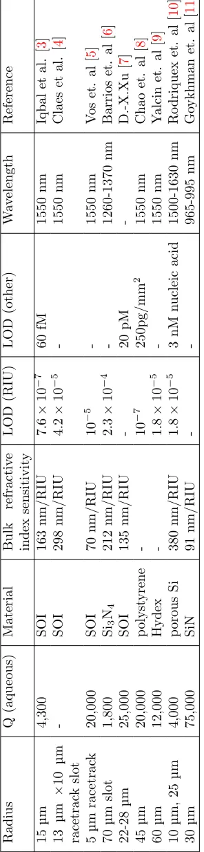
• Geometry parametersThe main geometrical parameter of the ring is its radiusr. A small radius will introduce bend losses which increase radiation and lower the overall Q. At the same time, a larger radius will increase the interaction of the mode with the side walls, and increase scattering losses. Various geometries have been used in order to increase the overlap of the mode with the analyte of interest. Some groups employ slot resonators, which allow the mode within the slot to interact with the solution of interest. Other groups have employed porous Si as the resonator material, which allows the particles/molecules of interest to enter the pores and interact with the mode. However, the addition of the extra surfaces of the pores can lower the Q-factor through scattering losses.

The performance metrics commonly used to characterize the sensor are:

• The sensitivity (S), represents the change in resonant frequency per change of index of

refraction of the bulk solution. It is determined by the light-matter interaction, and depends on the fraction of the optical mode that interacts with the analyte. There is a trade-off between increased sensitivity and high Q-factor; the more the mode is pushed outward, the better the sensitivity, but the higher the absorption losses within the surrounding medium.

• The limit of detection (LOD) represents the smallest change that can be discriminated.

It is defined as:

LOD = 3σ S ,

where S is the sensitivity andσis the standard deviation of the baseline signal.

There have been a multitude of experiments and designs of WGM resonators. Some of the geometries employed and their performance metrics are shown in Table2.1.

(29)

(30)

(31)

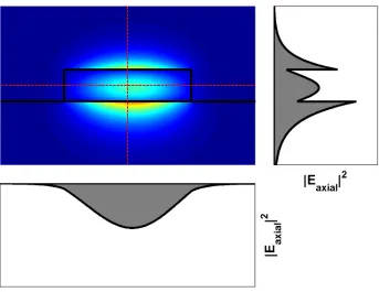
Figure 2.3: Mode profile along a vertical section through the center of resonator. The different colors indicate the different media through which the mode propagates. By fitting a decaying exponential to the tail of the evanescent field inside water, we obtain a decay constant of 160 nm.

stoichiometric Si3N4 (Rogue Valley Microdevices, Medford, OR) on top of a thermally grown oxide

layer. The height of the Si3N4is 250 nm±5%, and the height of the SiO2is 6µm±5%. The nitride

is deposited by chemical vapor deposition using dicholorosilane (SiH2Cl2) and ammonia (NH3) in

a horizontal vacuum furnace at a temperature of 800◦C. The refractive index at λ = 632 nm is 2.00±0.05. The substrate is a bare P/Boron doped, h100isilicon wafer. The mode profiles in the ring are simulated and displayed in Figure2.2. The simulated FSR of the ring was determined to be FSR = 343 GHz in water, which is comparable to our laser scanning range of 400 GHz.

The electromagnetic energy confined to the ring exhibits an evanescent tail that interacts with the surrounding medium of the ring (see Figure2.3). The evanescent tail probes the index of refraction of the surrounding medium; variations in the upper cladding affect the resonance frequency of the ring. If we introduce a solution with an unknown index of refraction, we can monitor the change in resonance frequency and derive the actual concentration of solute. The resonator responsivity is calibrated by exposure to known concentrations of the same solute. Blind experiments confirm the validity of the calibration steps. Similarly, a target molecule that binds to the ring resonator affects the index of refraction of the upper cladding and produces a quantifiable resonance shift. Models of the binding kinetics in conjunction with calibration steps enable us to determine the bulk concentration of the target molecule.

(32)

Figure 2.4: a) The evanescent tail of the mode interacts with a bulk solution b) The evanescent tail of the mode interacts with a surface organic layer.

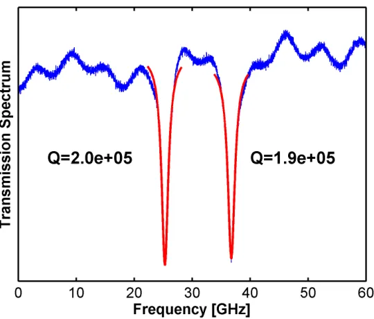
Figure 2.5: RecordedQ-factors of two fabricated rings coupled to the same waveguide.

both ring and disk resonators. The disks have higher Q-factors because of the lack of the interior boundary wall which reduces scattering losses. However, the spectrum of the disk is crowded by multiple resonances, which complicates tracking of individual resonances. Therefore, we employ ring resonators in our experiments. The fabrication yields highQ-factors, on the order of 105 _{in water.}

In Figure2.5 we show Q-factors of two resonators that are coupled to the same waveguide. Both resonators haveQ≈2×105_{, and the resonances are spaced by 12 GHz. The spurious oscillations in}

(33)

Figure 2.6: a) SEM picture of the ring resonator geometry b) SEM picture of the coupling region between the bus waveguide and the ring resonator. Pictures courtesy of Dongwan Kim.

2.2

Response to bulk and surface chemistry: simulations and

experiment

To quantify the performance of our resonators, we determine the resonance shift due to changes in the bulk index of refraction of the upper cladding, and to the deposition of a thin layer of organic material on top of the resonator. We estimate the magnitude of these shifts using COMSOL MultiplysicsTM_{. The finite element method (FEM) simulations are based on the weak formulation}

of the Maxwell equations, and make use of the axial symmetry of the ring resonators, following a method developed by Oxborrow [13,14]. Briefly, the Helmholtz equation

∇ ×(1

∇ ×H) = ω

c 2

H

is solved for the H-field, given an initial guess of the azimuthal mode number M. If the resulting resonant frequency is within a 400 GHz window of the nominal wavelength of 1064 nm, the solution has been found. Due to the simulated 343 GHz FSR of the ring, we expect to find at least one such resonance in our laser scanning range. If no such frequency is encountered, the guess forM is incorrect, and we rerun the simulation with an updated value forM.

2.2.1

Salt titrations

(34)

Figure 2.7: a) Change in resonant frequency as a function of salt concentration, for a ring resonator with waveguide height ofh= 250 nm and ring width ofw= 1µm.

expressed as mass percentage (the mass of the solute over the total mass of the solution) [15, 16]. This relationship was determined at 1550 nm and temperatures of 18◦C, 25◦C and 45◦C; we assume it true at 1064 nm as well.

Initially, FEM simulations determined the expected resonance shift for concentrations of NaCl up to 200 mM. We set the upper cladding index to be the index of refraction of waternH2O= 1.324, and determine the azimuthal mode number M that results in a resonance wavelength within the scanning range of our laser. With the previously determinedM, we change the index of refraction of the upper cladding layer with varying concentrations of NaCl, and track the resonance wavelength. We record the resulting resonance frequency, and plot the change in resonance frequency as a function of the molarity of the salt solution (see Figure2.7). Linear regression reveals a sensitivity to bulk refractive index of 72.7 nm RIU−1_{, or, alternatively,} _{−19.3 THz RIU}−1_.

2.2.2

Organic layer

(35)

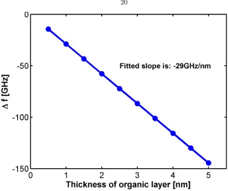
Figure 2.8: Change in resonant frequency as a function of the thickness of the organic layer.

resonator, the thickness and density of the organic layer changes the effective index of the mode. The organic molecules have an index of refraction (n≈1.45) that is higher than the index of refraction of the water molecules they displaced (n≈1.33).

Starting from the equation M λ= 2πRneff, and assuming small perturbations, the wavelength

shift can be expressed as:

∆λ= 2πR ∂neff ∂nupper

∆nupper= 2πRΓupper∆nupper.

The term Γupper is known as the confinement factor, and represents the fraction of the optical

field intensity of the mode that is located in the upper cladding. Confinement factors for the lower cladding, Γlower, and for the core, Γcore, are similarly defined. The confinement factor for the organic

layer has the form:

Γorg=

R

orgnorg|E(r)| 2_d3_r

neffR |E(r)|2d3r

. (2.1)

We use perturbation theory to determine Γorg, assuming that the deposition of the thin organic layer

does not affect the magnitude and distribution of the electric field. COMSOL simulations provide the mode profile assuming a water upper cladding, from which we extract the electric field in a thicknessdat the top and sides of the resonator, and calculate Γorg using Eq.(2.1). The deposition

(36)

neff of ∆neff = Γorg∆nupper. Writing the resonance condition in terms of frequencyf, M c f

= (2πR)neff,

the frequency shift due to a small change in the index of refraction of the upper cladding, nupper,

becomes

∆f = −cMΓorg 2πRn2

eff

∆nupper.

Figure 2.8shows the variation in the frequency shift with thickness of the deposited organic layer; the resulting sensitivity is 29 GHz nm−1_.

2.3

Noise sources

2.3.1

Temperature

Thermal noise is the prevalent noise source. One approach to reduce noise due to macroscopic temperature variations is to design an athermal device that allows the thermal effects in the different cladding and core media to cancel each other; this degree of control is difficult to maintain over a large range of upper cladding indexes. The response of the sensor to changes in temperature can be determined from the resonance conditionmλ= 2πRneff,i.e.,

∂λ ∂T =

2π m

_∂R

∂Tneff+R ∂neff ∂T = 2πR m αneff+

∂neff

∂T

=λ

α+ 1 neff

∂neff

∂T

,

where α= (∂R/∂T)/Ris the coefficient of thermal expansion of Si3N4, α= 3.27×10−6/◦C. The

change∂neff/∂T can be further expanded to consider the roles of the different media:

∂neff ∂T = _∂n ∂T core

Γcore+

_∂n

∂T

lower

Γlower+

_∂n

∂T

upper

Γupper,

∂neff

∂T = TOCcoreΓcore+ TOClowerΓlower+ TOCupperΓupper,

where we encounter, as before, the confinement factors Γ that represent the fraction of the modal energy inside each medium:

Γlayer=

R

layern(r)|E(r)| 2_d3_r

neffR|E(r)|d3r

.

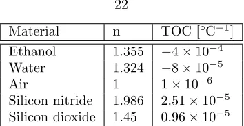
The values used for the indexes of refraction and the thermo-optic coefficients (TOCs) of different materials are summarized in Table2.2.

(37)

Air 0.06 0.75 0.19 659 1.594 -4.6 GHz/ C

Table 2.3: Calculated values of the confinement factors for three upper cladding media and the resulting temperature sensitivities.

sensitivity in ethanol is positive, ∆f /∆T = 4.5 GHz/◦C. The TOC of water is also negative, but it is smaller than that of ethanol; hence, the overall temperature sensitivity for water is negative, ∆f /∆T =−2.7 GHz/◦_{C. Lastly, air has a slightly positive TOC, so its temperature sensitivity is} more negative than water, ∆f /∆T =−4.6 GHz/◦_{C. Experimental calibrations of the temperature} response of the resonator in all three media will be discussed later in the chapter.

2.3.2

Pressure

Pressure variations affect the response of the sensors by mechanically altering the geometry of the ring. Indeed, Zhao et al. use arrays of ring resonators fabricated on deformable diaphragms as sensitive pressure transducers [17]. Changes in the ring shape due to mechanical forces alter the optical mode profile, producing resonance frequency shifts. In our platform, the fluid flow can deform the chip substrate, which has been thinned to enable accurate cleaving along the crystal planes. Later in this chapter we will show experimental pressure calibrations.

2.4

Dual resonator platform

Ring resonators are very sensitive transducers, but, as described above, they are also easily affected by environmental noise. A simple and effective way to remove the ambient noise (also known as common-mode noise) is to perform a differential measurement by introducing a second, reference resonator. Some groups are already using this differential measurement scheme in a geometry in which the reference resonator is covered with a cladding material, usually a polymer (see Table2.4

for details on polymer type and thickness).

(38)

Cladding material Thickness Reference

CYTOP 1.1µm Iqbal et al. [3]

SU-8 2µm Xu et al. [7]

TEOS 530 nm Gylfason et al.[18]

Table 2.4: Materials used for covering the reference resonator.

analyte stream since it is not in thermal and mechanical contact with the liquid. Second, the extra fabrication steps in depositing the cladding layer and etching a window over the sensing resonator can greatly reduce the fabrication yield. An optimization study has to be carried out to determine the optimal thickness of the cladding layer in order to minimize insertion losses. Third, the flow to the sensing resonator may be influenced by the 1µm-2µm thick polymer cladding, reducing mass transfer of the analyte to the sensor. Lastly, some groups report degradation of the cladding with time, in particular SU-8, as it absorbs water over time [7].

To eliminate these drawbacks, reduce the noise floor, and simplify the device fabrication, we introduce a platform in which the reference resonator and the sensing resonator share a common microfluidic channel, through which both are exposed to the fluid flow. Due to the small dimensions of the channel, the flow is viscous, so convection dominates over diffusion. This enables us to flow two streams, one with the chemical of interest, the other with a reference buffer, side-by-side without mixing. Thus, the sensing resonator is exposed to the solution of interest, while the reference resonator is immersed in the reference buffer. This allows both the pressure and temperature of the fluid to equilibrate, enabling the reference resonator to account for those noise sources as well.

2.4.1

Concentration and temperature equilibration

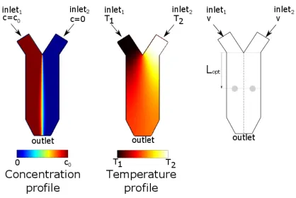
First, we must prove that including the two resonators in the same channel does not induce mixing of the streams that would foul our analyte. For a concentrationc0 at one inlet, and a concentration

c= 0 at the buffer inlet, COMSOL simulations predict concentration and temperature variations in the diffusion zone shown in Figure2.9.

Because convection dominates over diffusion for large solute molecules, the molecules are swept downstream before they can diffuse to the resonators. The diffusion length δc = 2√Dct represents

a characteristic length over which the analyte has propagated in time t. Assuming an average velocity in the channel ofvavg= 1 mm s−1, with the resonators locatedL= 1 mm downstream from

the beginning of the common channel, the diffusion length will be δc ≈ 20µm for a solute with

diffusivityDc= 10−10m2s−1. Because the resonators are separated by 800µm, mixing between the

two streams is, indeed, negligible.

Like species diffusion, the temperature diffusion length grows as δt = 2√Dtt, where Dt is the

(39)

Figure 2.9: Equilibration of concentration and temperature inside the channel

1.43×10−7_m2_s−1 _{for water at 25}◦_{C. For a location}_L_{= 1 mm downstream, the thermal diffusion} length becomesδth ≈750µm. Thus, the two streams equilibrate thermally, without species mixing.

2.4.2

Sensitivity to geometric parameters

Even when performed with great care, the fabrication of the resonator will lead to deviations from the ideal design parameters. Here we examine the influence of these variations on the response of the resonator, paying particular attention to the effects of small changes in the waveguide height and ring width of the resonator. These variations in the geometrical parameters of the sensing and reference ring lead to different responses to temperature, pressure and concentration changes. On one hand, such variations are desirable because the transmission spectrum will exhibit two separate resonances, simplifying identification and tracking of the two signals since they do not overlap. On the other hand, the responses of the two resonators will differ, as their differential signal will not exactly cancel. Because the two resonators are in close proximity, these fabrication variations should be fairly small.

(40)

Figure 2.10: a) Resonant frequency as a function of waveguide height b) Resonant frequency as a function of ring width.

of the ring from 240 nm to 250 nm in steps of 1 nm. We also vary the width of the ring from 0.98µm to 1.02µm in steps of 10 nm. The radius of 70µm of the ring was fixed while varying the width. Figure2.10shows the predicted variation in resonance frequency in water for small changes around a base geometry of height 250 nm and width 1µm. The changes in resonant frequency have a slope of 149 GHz/nm for changes in the height of the resonator, and 14 GHz/nm for changes in the radius of the resonator. The azimuthal modeM is constant along the dotted lines in the figure, and increases by 1 for adjacent lines. As a consequence, we cannot determine if the two resonators have the same M.

Since one cannot determine M from the transmission spectrum, one must question whether the differences in the sensing and reference responses influence the sensitivity of the ring resonator plat-form. We have previously estimated the bulk sensitivity of our base geometry to be 72.7 nm RIU−1_.

Figure 2.11 shows that despite variation in the geometrical parameters and the correspondingly

(41)

Figure 2.12: a) Sensitivity to surface sensing as a function of ring height b) Sensitivity to surface sensing of as a function of ring width.

Figure 2.13: a) Temperature sensitivity as a function of waveguide height b) Temperature sensitivity as a function of ring width.

different M values, the sensitivity still changes linearly with resonator height and width. Setting an upper bound on the geometry variation of two adjacent rings of 5 nm for the height and 10 nm for the width, we derive an upper bound on the sensitivity variation for bulk refractive indexes of 2 nm RIU−1 _{and 0.5 nm RIU}−1_{, respectively.}

A similar analysis for the response to a layer of organic thickness, shown in Figure2.12, yielded upper bounds of 0.6 GHz nm−1 _{and 0.09 GHz nm}−1_{. The temperature response is well described by}

linear fits of sensitivity to changes in geometric parameters, as shown in Figure2.13. The derived upper bounds are 0.06 GHz◦C−1 _{and 0.01 GHz}◦_C−1_.

(42)

2.4.3

Experimental setup

The setup consists of a 1064nm vertical-cavity surface-emitting (VCSEL) based optoelectronic lin-early swept frequency laser that scans a frequency range of 400 GHz in a time span of 2 ms. The linear frequency sweep simplifies the identification and tracking of the resonant frequencies, and its high scan speed allows for high time resolution measurements. For a more detailed description of the laser, see [12]. The laser is coupled into the resonator chip from free space optics, and the output beam is aligned to a photodetector connected to an oscilloscope (Figure2.14). The resonant frequencies are identified by fitting two Lorentzian lineshapes to the transmission spectrum. The resonator chip itself is comprised of the silicon nitride wafer, in which the ring resonators are etched, and a polydimethylsiloxane (PDMS) chip on top, with defined flow channels for liquid delivery. The flow platform has four inlets from which we can select two by using elastomeric valves, each being delivered to the reference and sensing resonator in the common flow channel, and obey laminar flow conditions. We will describe the flow design and mode of operation of the microfluidics in more detail in Chapter 3. The chip is attached to a copper block using adhesive transfer tape. The copper block contains a thermistor that records the temperature of the stage and a Peltier thermo-electric cooler through which the temperature of the stage is computer-controlled and monitored.

To exemplify the achievement of laminar flow, we introduce two colored dyes in the common channel. In Figure2.15we show the separation of the two streams.

(43)

2.4.4

Experimental results

2.4.4.1 Bulk refractive index experiments

To demonstrate the sensing ability of our platform and determine its response to bulk refractive index changes, we perform sensing experiments with a range of concentrations of sodium chloride (NaCl), with the temperature of the chip fixed at T = 26◦C. Briefly, solutions of DI water are introduced from two inlets over the sensing and reference resonators to establish a baseline. Then, a solution of NaCl is introduced from one of the inlets over the sensing resonator. The last step is to reestablish the baseline, by flowing DI water over the sensing resonator. Differential shifts for concentrations of 2.5 mM, 5 mM, 10 mM, and 40 mM are displayed in Figure2.16. Between five and ten cycles of the same NaCl concentration are recorded. We determine a bulk index sensitivity of 72.6±0.3nm RIU−1_{, or, alternatively, 19.2}_{±0.1THz RIU}−1_{. These values are in excellent agreement}

with our simulated values of 72.7 nm RIU−1 _and_{−19.3 THz RIU}−1_.

(44)

Figure 2.17: Temperature calibrations in ethanol. The first subplot shows the actual temperature of the stage as recorded by the thermocouple. The second subplot shows the response of the sensing and reference resonators. The reference resonator response has been shifted upwards by 20 GHz for ease of visualization. The third subplot shows the differential signal. Note that the scale for the differential signal is 20 times smaller than that for the individual responses.

2.4.4.2 Temperature calibration experiments

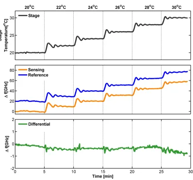
The temperature of the stage was controlled and monitored using a temperature controller (New-port, LDC-3724). The temperature was changed in increments of ∆t = 2◦C, after which the new temperature was maintained for 5 min or 6 min, to allow the resonator response to stabilize. Oscilla-tions in both the temperature and resonator responses result from slow feedback in the temperature stabilization.

(45)

Figure 2.18: Temperature calibrations in water. The first subplot shows the response of the sensing and reference resonators. The reference resonator response has been shifted upwards by 2 GHz for ease of visualization. The second subplot shows the differential signal, on a scale 6 times smaller.

and show similar trends, whereas the differential signal is mostly insensitive to the temperature fluctuations. The standard deviation of the differential signal isσ= 183 MHz. Least squares fitting of the individual response to the stage temperature,Ts, reveals the temperature sensitivity of each resonator,Ri, to the form:

Ri≈ai×Ts+bi,

which yieldsa1=a2= 6.1 GHz/◦C for both resonators in ethanol. These values are higher than the

simulated value in the previous section of 4.5 GHz/◦C.

Two temperature calibration experiments were also performed in water. In the first experiment, shown in Figure 2.18, the temperature was ramped up and down between 26◦C and 30◦C. We again fit the recorded stage temperature to each resonator response and we extract sensitivities of a1=a2=−0.5 GHz/◦C. The standard deviation of the differential signal isσ= 175 MHz. A second

experiment in water involves ramping the temperature from 22◦C to 32◦C, with similar results, shown in Figure 2.19. The extracted sensitivity is a1 =a2=−0.6 GHz/◦C. The simulated values

for the temperature sensitivity in water are−2.7 GHz/◦_{C, larger than the measured ones.}

(46)

Figure 2.19: Temperature calibrations in water. The first subplot shows the stage temperature cycles. The second subplot shows the response of the sensing and reference resonators. The reference resonator response has been shifted upwards by 2 GHz. The third subplot shows the differential signal.

The measurement temperature sensitivities are not in agreement with the simulated values. A possible explanation is that the recorded stage temperature is not an accurate estimate of the temperature at the resonator since the introduced fluids are at room temperature, and they could lower the temperature experienced by the resonator. Despite this disagreement, the overarching conclusion is that the differential signal is insensitive to temperature variations in the three media, proving the viability and sensing capabilities of our platform.

(47)

Figure 2.20: Resonator response to cycles of 40 mM NaCl in a temperature varying environment. Temperature shifts affect the individual resonator responses, but not the differential signal.

responses to a concentration of 40 mM of NaCl. The temperature variations are apparent in the individual resonator responses, but not the in differential signal. From similar experiments involving the four concentrations mentioned above, we extract a bulk sensitivity of 62.4±0.9nm RIU−1_{, or,}

alternatively, 17.0±0.2THz RIU−1_{. The standard deviation of the baseline signal is} _σ

baseline =

80 MHz, which leads to a limit of detection LOD = 3σbaseline/S= 1.4×10−5RIU.

2.4.4.3 Presssure calibration experiments

(48)

(49)

σ_y2(nτ) =1 2

*" 1 n

n−1

X

i=0

(fi+n−fi) #2+

,

whereτ is the time interval between successive sample points,nis the number of samples averaged, andfi the response of the resonator at timeiτ.

We plot the Allan deviation for integration times from 10 s to 30 min, corresponding to typical durations for an experiment. For the results to be statistically significant, data were collected for at least 4 h, a factor of 8 higher than our maximum integration time. To compare the noise in our dual laminar platform to that in a platform in which the reference resonator is covered, we fabricated devices in which the reference resonator is covered by a 6µm layer of SU-8 (shown in Figure2.22).

Figure 2.22: a) Dual-flow platform. b) Covered reference ring platform.

(50)

Figure 2.24: a) Allan deviation in air.

(51)

R. C. Bailey, and L. C. Gunn, “Label-free biosensor arrays based on silicon ring resonators and high-speed optical scanning instrumentation,” IEEE Journal of Selected Topics in Quantum Electronics, vol. 16, pp. 654–661, May 2010.

[4] T. Claes, J. G. Molera, K. D. Vos, E. Schacht, R. Baets, and P. Bienstman, “Label-free biosens-ing with a slot-waveguide-based rbiosens-ing resonator in silicon on insulator,”IEEE Photonics Journal, vol. 1, pp. 197–204, Sept 2009.

[5] K. D. Vos, I. Bartolozzi, E. Schacht, P. Bienstman, and R. Baets, “Silicon-on-insulator microring resonator for sensitive and label-free biosensing,”Opt. Express, vol. 15, pp. 7610–7615, Jun 2007.

[6] C. A. Barrios, K. B. Gylfason, B. S´anchez, A. Griol, H. Sohlstr¨om, M. Holgado, and R. Casquel, “Slot-waveguide biochemical sensor,”Opt. Lett., vol. 32, pp. 3080–3082, Nov 2007.

[7] D.-X. Xu, M. Vachon, A. Densmore, R. Ma, A. Delˆage, S. Janz, J. Lapointe, Y. Li, G. Lopinski, D. Zhang, Q. Y. Liu, P. Cheben, and J. H. Schmid, “Label-free biosensor array based on silicon-on-insulator ring resonators addressed using a wdm approach,” Opt. Lett., vol. 35, no. 16, pp. 2771–2773, 2010.

[8] C.-Y. Chao, W. Fung, and L. J. Guo, “Polymer microring resonators for biochemical sensing applications,”IEEE Journal of Selected Topics in Quantum Electronics, vol. 12, pp. 134–142, Jan 2006.

[9] A. Yalcin, K. C. Popat, J. C. Aldridge, T. A. Desai, J. Hryniewicz, N. Chbouki, B. E. Little, O. King, V. Van, S. Chu, D. Gill, M. Anthes-Washburn, M. S. Unlu, and B. B. Goldberg, “Optical sensing of biomolecules using microring resonators,”IEEE Journal of Selected Topics in Quantum Electronics, vol. 12, pp. 148–155, Jan 2006.

[10] G. A. Rodriguez, S. Hu, and S. M. Weiss, “Porous silicon ring resonator for compact, high sensitivity biosensing applications,”Opt. Express, vol. 23, pp. 7111–7119, Mar 2015.

(52)

[12] J. B. Sendowski,On-chip integrated label-free optical biosensing. PhD thesis, California Institute of Technology, 2013.

[13] M. Oxborrow, “How to simulate the whispering-gallery modes of dielectric microresonators in FEMLAB/COMSOL,” in Lasers and Applications in Science and Engineering, pp. 64520J– 64520J, International Society for Optics and Photonics, 2007.

[14] M. Oxborrow, “Traceable 2-D finite-element simulation of the whispering-gallery modes of ax-isymmetric electromagnetic resonators,”Microwave Theory and Techniques, IEEE Transactions on, vol. 55, no. 6, pp. 1209–1218, 2007.

[15] J. R. Zhao, X. G. Huang, and J. H. Chen, “A Fresnel-reflection-based fiber sensor for simul-taneous measurement of liquid concentration and temperature,” Journal of Applied Physics, vol. 106, no. 8, 2009.

[16] H. Su and X. G. Huang, “Fresnel-reflection-based fiber sensor for on-line measurement of solute concentration in solutions,”Sensors and Actuators B: Chemical, vol. 126, no. 2, pp. 579 – 582, 2007.

[17] X. Zhao, J. M. Tsai, H. Cai, X. M. Ji, J. Zhou, M. H. Bao, Y. P. Huang, D. L. Kwong, and A. Q. Liu, “A nano-opto-mechanical pressure sensor via ring resonator,”Opt. Express, vol. 20, pp. 8535–8542, Apr 2012.

(53)

On-chip valve technology for

reducing response time

This chapter presents and characterizes a design for the fluidic network that delivers the solutions to the resonators, with a focus on reducing the response time of the platform. The channels that en-capsulate the ring resonators are made of polydimethylsiloxane (PDMS), an elastomer that has been widely used in microfluidics because it is easily moldable, low-cost, gas-permeable and transparent. Most importantly, PDMS is excellent for rapid prototyping of new designs and has the advantage that elastic valves can be manufactured using a bi-layer design [1,2]. Other materials from which fluidic chips are fabricated include polymethylmethacrylate (PMMA) and Mylar plastic, but, due to their rigidity, they cannot support on-chip valves, and their fabrication is complex. Designs of the fluidic network require careful choices of the dimensions of the channel, the driving force of the flow, and the method of switching the flow that is delivered to the resonator between a buffer and the analyte of interest. The switching method strongly influences the response time of the system. The range of volumetric flow rates and channel dimensions are summarized in Table3.1.

Syringe pumps that can operate in either the infusion or the withdrawal mode are commonly used to drive the flow to the resonator chip. In our first experiments, we also used programmable syringe pumps together with a three-way solenoid valve to drive the flow to the resonators, and to switch the fluid streams, as shown in Figure3.1. Briefly, either one of the two top syringes can drive the flow over the sensing resonator, depending on the setting of the three-way solenoid valve. A third syringe pump containing buffer solution drives the flow over the reference resonator.

(54)

Material Channel dimen-sions

Flow rates Switching Mecha-nism

Reference

Mylar 175µm ×500µm 5, 10, 30

µl min−1

robotic arm for plate aspiration

Iqbal et al [3]

PDMS 20µm×200µm 10µl min−1 _in-line _injector

valves

Gylfason et al. [4]

PDMS 50µm×200µm 5µl min−1 - DeVos et al [5]

PDMS - 10µl min−1 manual Grist et al [6]

Table 3.1: Various geometries of the fluidic channels and flow characteristics employed by different groups.

Figure 3.1: Initial setup that includes syringe pumps and a three-way solenoid valve to control the flow to the resonator chip. Two syringe pumps containing the buffer (blue) and the analyte of interest (orange) are connected to the three-way solenoid valve, which is computer-controlled. We can switch the flow from either of the first two syringe pumps and direct it to the sensing resonator. A third syringe pump with buffer (blue) is continuously flowing to the reference resonator.

the dual-laminar flow platform when a 172 mM NaCl solution is introduced using the syringe pump setup. First, we flow deionized (DI) water over both the sensing and reference resonators for 15 min to establish the baseline signal. Then, we switch the flow at the three-way solenoid valve from water to salt. Two characteristics of the response to the switch are apparent in Figure3.2: first, there is a delay between the time the switch occurs at the three-way solenoid valve and that when a change in the resonator response is first detected. This delay time oftdelay≈10 min results from the transport

(55)

Figure 3.2: Salt sensing using solenoid and syringe pumps. The areas shaded in red represent the delay between the switch of the flow at the three-way solenoid valve and the presence of a change in the resonator response. The areas shaded in blue represent the transient phase of the response.

flowing salt, we re-establish the baseline by switching the sensing flow to water. We notice a similar tdelay and attransient in re-establishing the baseline. A theoretical model that predicts the observed

behavior of the response in this setup is presented at the end of the chapter.

Due to these delays and transient times, a bulk sensing experiment aimed at measuring a given concentration requires a few hours of data collection. To reduce the response time, we must reduce the dead volume in the flow system. To that end, we introduce a microfluidic platform in which the switching of the flows happens immediately upstream of the common resonator channel, on the same chip as the rings. This is achieved by using two-layer microfluidic chips with integrated elas-tomeric valves. Briefly, the elaselas-tomeric valves are channels in the top PDMS layer that expand when pressurized, restricting the flow in any channel in the bottom layer directly below and perpendicular to the valve. The top of bottom channel is rounded in the crossing zone to allow a complete seal. The top layer is referred to as the “control layer”, whereas the bottom layer is referred to as the “flow layer.” The thickness of the membrane between the two perpendicular channels is critical to the function of the valve. If the membrane is too thin, it will break under the fluid pressure, but if it is too thick, it will not deform enough to completely seal the flow channel. The choice of which control channel is pressurized can be determined using the manifold setup shown in Figure3.3

(56)

Figure 3.3: A schematic diagram of the fluidic control of the solutions delivered to the PDMS chip. Two regulators control the pressures for the control and flow layer. The control layer tubing is connected to a solenoid manifold that turns the valve for each control channel on or off.

reflow the polymer with a smooth fillet. However, in the first design used, a slight backflow into the adjacent channels was observed (see Figure3.4). Therefore, our second microfluidic design has valves right at the T-junction of two channels. The final design, shown in Figure3.5, has four inlets that are pressurized atp= 34 kPa (5 psi) and that are loaded with different solutions. Inlets 1