Stochastic Characterization of Strong Ground Motion and Applications to Structural Response

(1)

of Strong Ground Motion

and Applications to Structural Response

Thesis by

Konstantinos Papadimitriou

In Partial Fulfillment

of the Requirements for the Degree of Doctor of Philosophy

California Institute of Technology Pasadena, California

1991

(2)

(3)

Acknowledgments

I am deeply grateful to my advisor, Professor J.1. Beck, for his guidance and encouragement throughout the course of my research. His continuous availability and enthusiastic guidance are greatly appreciated.

I am sincerely grateful for the generous financial support provided to me by the California Institute of Technology, which made my studies here possible.

I would like to thank all my professors for the excellent education they offered me during my graduate studies. I also thank the people in Thomas who created a friendly environment, making my stay here a very pleasant experience.

My deepest thanks to Lambros Katafygiotis, Petros Koumoutsakos, and Roberto Camassa for the many memorable experiences we shared. The assistance of Suzette Martinez and Sharon Beckenbach with the typing of this thesis is greatly appreci-ated.

(4)

Abstract

This study addresses the problem of characterizing strong ground motion for the purpose of computing the dynamic response of structures to earthquakes. A new probabilistic ground motion model is proposed which can act as an interface between ground motion prediction studies and structural response studies. The model is capable of capturing, with at most nine parameters, all those features of the ground acceleration history which have an important influence on the dynamic response of linear and nonlinear structures, including the amplitude and frequency content nonstationarities of the shaking. Using a Bayesian probabilistic framework, a simple and effective statistical method is developed for extracting the "optimal" model from an actual accelerogram. The proposed ground motion model can be efficiently applied in simulations as well as analytical response and reliability studies of linear and inelastic structures.

The random response of linear and nonlinear oscillators subjected to the

(5)

Table of Contents

Acknowledgments Abstract . . . . Table of Contents

List of Tables and Figures Chapter 1: Introduction

1.1 Motivation and Objectives 1.2 Summary of this Study

111

IV .v

.X

. 1

1

3 Chapter 2: Modeling of Strong Ground Motion by Stochastic

Dif-ferential and Difference Equations . . . . 6 2.1 Introduction . . . 6 2.2 General Class of Strong Ground Motion Models 11

2.2.1 Continuous Model 12

2.2.2 Discrete Model . . 12

2.3 Subclasses of Strong Ground Motion Model 14

2.3.1 Stationary Stochastic Model . . 14

2.3.2 Piecewise Time-Invariant Model 17

2.3.3 Envelope-Modulated V/hite Noise Model 18 2.3.4 Piecewise Time-Invariant Frequency Content Model 19 2.4 Bayesian Methodology for Parameter Estimation . . . . 19 2.4.1 General AR(p) Model with Time-Varying Coefficients 20

2.4.2 Piecewise Time-Invariant Model 22

2.4.3 Envelope-Modulated White-Noise Model 23

2.4.4 Piecewise Time-Invariant Frequency Content Model 24 2.5 Structural Response and Ground Motion Model Adequacy 25

2.5.1 Nonlinear Hysteretic Model 25

2.5.2 Equation of Motion . . . . 26

2.5.3 Probabilistic Linear Elastic and Inelastic Response Spectra 28

(6)

2.6.1 Moving Time-Window Approach 30

2.6.2 Physical Interpretation of Time Variation of the Model Coe

f-ficients . . . 31 2.7 Modeling and Simulation of Earthquake Accelerograms 33

2.7.1 Modeling of the Intensity Using Various Models 34

2.7.2 Modeling of the Frequency Content Using PTIFC Models 35

2.7.3 Modeling of the Very Low Frequency Content 38

2.8 Conclusions

Chapter 3: Parsimonious Probabilistic Modeling of Strong

Ground Motion

3.1 Introduction . . . .

3.2 Stochastic Second-Order Differential Equations with Variable Coe f-ficients

3.2.1 Au to covariance Function

3.2.2 Evolutionary Power Spectral Density Function

3.2.3 Relation Between ACF and EPSD Function

3.3 Discrete Equation and Its Relation to the Continuous One

3.4 Parsimonious Ground Motion Model

40

64 64

65 65

68

69

71

3.4.1 Analysis and Simulation of Earthquake Accelerograms 74

3.4.2 Structural Response and Model Adequacy 75

3.5 Concluding Remarks . . . 76

Chapter 4: Transient Response Characteristics of Stochastically

Excited Linear and Nonlinear Systems . . . 89 4.1 Introduction . . . 89

4.2 Mathematical Formulation of the Response 91

4.2.1 Mean-Square Response 92

4.2.2 Covariance Response 93

4.2.3 Special Case: Modulated vVhite-Noise Excitation

4.3 Formulation for the Mean-Square Response of Linear Time Invariant

SDOF Oscillators

4.3.1 Mean-Square Displacement

93

(7)

4.3.2 Mean-Square Velocity . . . . 4.3.3 Mean-Square Absolute Acceleration 4.3.4 Displacement-Velocity Correlation

4.3.5 Similarities Between Transient and Stationary Mean-Square Response . . . .

4.3.6 Exact Solution for the Mean-Square Response

4.3.7 Exact Solution for the Covariance of the Response: Modu-lated "White-Noise Excitation

4.4 Approximation for the Mean-Square Response of a Linear

Time-96

97 97

97 98

99

Invariant SDOF Oscillator . . . " 99 4.4.1 Approximate First-Order Differential Equation for the

Mean-Square Displacement . . . . . 100 4.4.2 Accuracy of the Approximations using Modulated Whit

e-Noise Excitation . . . 101 4.5 Formulation for the Mean-Square Response of Nonlinear SDOF

Os-cillators . . . 105

4.5.1 Mean-Square Displacement 106

4.5.2 Mean-Square Velocity . . 107

4.5.3 Mean-Square Absolute Acceleration 107

4.5.4 Displacement-Velocity Correlation 108

4.5.5 Similarities Between Transient and Stationary Mean-Square Response . . . .. . . 108 4.6 Approximation of the Liapunov Matrix Equation for a Nonlinear

SDOF Oscillator 109

4.6.1 Covariance of the Response: Modulated White-Noise Excita-tion . . . 110 4.7 Approximation of the Forcing Integral Term of the Liapunov Matrix

Equation . . . 111 4.7.1 Broadband Excitation and Slowly-Varying Structural

Param-eters . . . 111

4.7.2 Lightly-Damped Oscillators 113

(8)

4.8.1 Modulated Filtered White-Noise Excitation 4.8.2 Filtered Modulated White-Noise Excitation

4.8.3 Stochastic Ground Motion Models

4.8.4 Accuracy of the Approximations Using the Proposed Stochas-114

116

tic Ground Motion Model . . . 120 4.8.5 Computational Aspects

4.9 Extension of the Approximations to Classically-Damped MDOF Lin-ear Systems

4.10 Conclusions

121

122 126

Chapter 5: Importance of Temporal Nonstationarity

In

the

Fre-quency Content of Ground Motion for Linear and N

on-linear Structural Models . . . 147 5.1 Introduction . . . 147

5.2 Description of EaJ-thquake Ground Motions 148

5.3 Linear SDOF Structural Model 149

5.4 Nonlinear SDOF Structural Model 152

5.4.1 Force-Deflection Relation 152

5.4.2 Equation of Motion Using the Equivalent Linearization

Method . . . . . 153 5.4.3 Characteristics of the Mean-Square Response; Moving

Reso-Chapter 6:

References

nance Effect Conclusions

Appendix A.I Solutions of Homogenous Second-Order Differential Equa-tion with Slowly-Varying Coefficients

Appendix A.2 Principal Matrix Solution . . . . .

Appendix A.3 Evolutionary Spectral Representation of a Stochastic Pro-154 170

173

179 181

cess . . . 182 Appendix B Relationships Between the Coefficients of Second-Order

Dis-crete and Continuous Equations 185

(9)

Appendix D Solution of the Second-Order Differential Equation Using the Two-Timing Method . . . 188 Appendix E Covariance Response of A Linear Oscillator Subjected to

Modulated White-Noise Excitation 191

Appendix F Complete Set of Equations for the Mean-Square

(10)

List of Tables and Figures

Figure 2.1. (a) Model I, (b) Model II, for ground acceleration.

Figure 2.2. Effect of n on the force-displacement curve [from Jayakumar, (1987)].

Figure 2.3. Hysteresis loop for periodic response of the structural model [from

Jayakumar, (1987)].

Figure 2.4. Force-displacement curves for arbitrary loading of the structural model

[from Jayakumar, (1987)].

Figure 2.5. Schematic diagram of a SDOF structure.

Figure 2.6. Acceleration time histories for the six accelerograms in Table 2.1.

Figure 2.7. Time variation of the frequency content of the accelerograms in Table

2.1, plotted in terms of the undamped frequency WI (solid), bandwidth

W1(1 (dashed-dotted) and damping ratio (1.

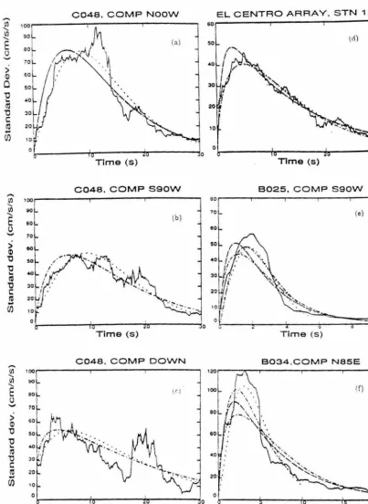
Figure 2.8. Comparison of the standard deviation computed for the accelerograms in Table 2.1 by the moving time-window approach (solid) and by the envelope-modulated white-noise model for the functions (2.1)

(dashed-dotted), (2.2) (dashed) and (2.58) (dotted).

Figure 2.9. The transformed series of stationary intensity for the NOOW component of the C048 record.

Figure 2.10. The NOOW component and one simulation for each optimal model of different subclasses. (a) "Target" accelerogram. (b) and (c) TIFC models with p=2 and p=4, respectively. (d) and (e) PTIFC models with p=2 and p=4, respectively.

(11)

compo-nent for each optimal model in Figure 2.10.

Figure 2.12. Comparison between the 5% damped response spectra of the "target" accelerogram (solid line), the mean response spectra (dashed-dotted

line) and the probabilistic response spectra (dashed lines which from

top to bottom correspond to p =0.99,0.90,0.50,0.10,0.01) computed for each optimal model in Figure 2.10. (a) and (b) correspond to

time-invariant frequency content models with p=2 and p=4, respectively.

(c) and (d) correspond to piecewise time-invariant models with p=2

and p=4, respectively.

Figure 2.13. Comparison between the 5% damped response spectra of the "target" accelerogram (solid line), the mean response spectra (dashed-dotted line) and the probabilistic response spectra (dashed lines which from top to bottom correspond to p =0.99,0.90, 0.50,0.10, 0.01) computed for the optimal PTIFC AR(2) model given in Table 2.2.

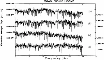
Figure 2.14. The Fourier transform of the "white-noise" samples in Figure 2.11.

Figure 2.15. Schematic diagram of the earthquake model, including Brune's source

model.

Figure 2.16. Power spectral density of the AR(p) model (dashed-dotted curved) and

the combined AR(p) and Brune's model (solid curve).

Figure 2.17. Comparison between the 5% damped acceleration response spectra

of the "target" accelerogram (solid line), the mean response spectra ( dashed-dotted line) and the probabilistic response spectra (dashed lines which from top to bottom correspond to p =0.99, 0.90, 0.50,

0.10,0.01) computed for optimal PTIFC AR(2) model in Figure 2.10,

including Brune's source model. (a) 0.04-20s period, (b) 0.1-2s period.

(12)

accelerogram (solid line), the mean response spectra (dashed -dot ted

line) and the probabilistic response spectra (dashed lines which from

top to bottom correspond to p =0.99, 0.90, 0.50, 0.10, 0.01) computed for optimal PTIFC AR(2) model in Figure 2.10, including Brune's

source model. (a) Velocity, (b) Displacement.

Figure 2.19. Comparison between the inelastic response spectra of the "target"

ac-celerogram (solid line), the mean response spectra (dashed-dotted line)

and the probabilistic response spectra (dashed lines which from top to

bottom correspond to p =0.99, 0.90, 0.50, 0.10, 0.01) computed for

optimal PTIFC AR(2) model in Figure 2.10, including Brune's source

model. Structural parameters n = 3, ry = 0.3 aJld ( = 0.05. (a) Acceleration, (b) Velocity.

Figure 2.20. Comparison between the inelastic response spectra of the "target"

and the probabilistic response spectra (dashed lines which from top to

bottom correspond to p =0.99, 0.90, 0.50, 0.10, 0.01) computed for optimal PTIFC AR(2) model in Figure 2.10, including Brune's source

model. Structural parameters n = 3, ry

=

0.3 and ( = 0.05. (a) Ductility, (b) Residual Ductility.

Table 2.1. List of some representative accelerograms for assessmg stochastic

ground motion model.

Table 2.2. Various technical information about the accelerograms in Table 2.1 for

PTIFC modelling.

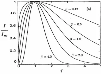
Figure 3.1. (a) Nondimensional time variation of the ground motion intensity for

different values of fl. (b) Relation between the nondimensional

dura-tion and

fl

for A = 10 and A = 20.

(13)

band-width wg(g (dashed-dotted curves), damping ratio (g, and (b)

inten-sity [g obtained by the nine-parameter model (smooth curves) and the

moving time-window approach (other curves) for the C04S.1 record in

Table 2.1.

Figure 3.3. Comparison of (a) the C04S.1 accelerogram and (b), (c) two artificial

accelerograms.

Figure 3.4. Time variation of (a) undamped frequency Wg (solid curves),

band-width wg(g (dashed-dotted curves), damping ratio (g, and (b)

inten-sity [g obtained by the nine-parameter model (smooth curves) and the

moving time-window approach (other curves) for the El Centro Array,

Stn 12 record in Table 2.1.

Figure 3.5. Comparison of (a) the El Centro Array, Stn 12 accelerogram and (b),

( c) two artificial accelerograms.

Figure 3.6. Comparison of the exact (solid curve) and approximate (dashed-dotted

curve) autocorrelation function

Ryy(t, s)

of the stochastic process

mod-eling the C04S.1 accelerogram.

Figure 3.7. The EPSD function plotted at different times (a) C04S.1, (b) El Centro

Array, Stn 12.

Figure 3.S. Comparison between the 5% response spectra of the C04S.1

accelero-gram (solid line), the mean response spectra (dashed-dotted line) and

the probabilistic response spectra ( dashed lines which from top to

bot-tom correspond to p =0.99, 0.90, 0.50, 0.10, 0.01) computed for the

nine-parameter optimal model.

Figure 3.9. Comparison between the inelastic response spectra of the C04S.1

(14)

bottom correspond to p =0.99,0.90,0.50,0.10,0.01) computed for the

nine-parameter optimal model. Structural parameters n

=

3, 1]

=

0.3,

and ( = 0.05.

Figure 4.1. N umber of cycles of oscillations needed for the oscillatory term to decay

to

n%

of its maximum value. n=l (solid curve), n=5 (dashed-dotted

curve), n= 1 0 (dot ted curve).

Figure 4.2. (a) Comparison between the nondimensiona.l exact (dashed curve) and

approximate (solid curve) mean-square displacement response of a

lin-ear SDOF oscillator subjected to a modulated (dashed-dotted curve)

white-noise excitation. 17 =

-¥o-

= 5.0.

Figure 4.2. (b) Comparison between the nondimensional exact (dashed curve) and

white-noise excitation. 17 = ~ = 2.0.

Figure 4.2. (c) Comparison between the nondimensional exact (dashed curve) and

white-noise excitation. 1] =

-¥o-

= 1.0.

Figure 4.2. (d) Comparison between the non dimensional exact (dashed curve) and

approximate (solid curve) mean-squa.re displacement response of a

white-noise excitation. 1] = ~ = 0.5.

Figure 4.3. (a) Time variation of normalized mean-square displacement, C12, 1022,

and Ea for different damping ratios. (3 = 0.5, 1] = 5. Dotted curve

corresponds to the time variation of the input modulation.

(15)

and Ea for different damping ratios. (3

=

0.5, 'r/

=

1. Dotted curve corresponds to the time variation of the input modulation.

Figure 4.3. (c) Time variation of normalized mean-square displacement, E12, E22,

and Ea for different damping ratios. (3 = 4, 'r/ = 5. Dotted curve corresponds to the time variation of the input modulation.

Figure 4.3. (d) Time variation of normalized mean-square displacement, E12, E22, and Ea for different damping ratios. (3

=

4, 17

=

1. Dotted curve corresponds to the time variation of the input modulation.

Figure 4.4. Approximate nondimensional mean-square displacement (solid curves)

of the response of a linear SDOF oscillator subjected to a modulated (dashed-dotted curve) white-noise excitation.

Figure 4.5. Contour plots of the fractional error EL as defined III (4.112). The excitation is modeled by MODEL 1.

Figure 4.6. Contour plots of >'

(w

o)

as defined in (4.94). The excitation is modeled

by MODEL 1.

Figure 4.7. Time variation of (a) the standard deviation and (b) the damped-frequency of the nine-parameter earthquake model fitted to the Orion

Blvd. recording.

Figure 4.8. Comparison between the exact (solid curve) and approximate (dashed curve) mean-square displacement response of a linear SDOF oscillator with 5% damping and Wo = 7,5,3, 1Hz. The excitation is the nine-parameter model shown in Figure 4.7.

Figure 4.9. Artificially designed time variation of the standard deviation and the damped-frequency of the nine-parameter excitation model.

(16)

curve) mean-square displacement response of a linear SDOF oscillator

with 5% damping and Wo = 7,5,3, 1Hz. The excitation is the

nine-parameter model shown in Figure 4.9.

Figure 4.11. Comparison between the exact (solid curve) and approximate

(dashed-curve) response of an equivalent linear SDOF oscillator. (a) STD of

the response (b) structural frequency

w(t).

Wo = 5Hz, (0 = 0.05.

The excitation is the nine-parameter model shown in Figure 4.7 whose

damped frequency variation is repeated again in (b).

Figure 4.12. Comparison between the exact (solid curve) and approximate

(dashed-curve) response of an equivalent linear SDOF oscillator. (a) STD of

the response (b) structural frequency

w(

t).

Wo

=

1Hz, (0

=

0.05. The excitation is the nine-parameter model shown in Figure 4.7 whose

damped frequency variation is repeated again in (b).

Figure 4.13. Comparisons between the exact (solid curve), the proposed

approxi-mate (dashed curve), and Bucher's approximate (dashed-dotted curve)

solution for the covariance response of two modes i and j.

f3

= 0.5,

(= 0.02.

Figure 4.14. Comparisons between the exact (solid curve), the proposed

approxi-mate (dashed curve), and Bucher's approximate (dashed-dotted curve)

solution for the covariance response of two modes i and j.

f3

= 0.5,

( = 0.05, w = 1Hz.

Figure 5.1. Time variation of ( a) the standard deviation

.;q;rt5

and (b) the

domi-nant frequency w~(t) for the (TV) and the (TI) excitation models fitted to the Orion Blvd. record shown in Figure 2.1(a).

Figure 5.2. Nonstationary linear response characteristics computed for the (TV)

(solid curves) and for the (TI) excitation (dashed-dotted curves) for

(17)

Figure 5.3. Comparison of (a) the r.m.s. displacement responses and (b) the equiv-alent linear structural frequencies, for the (TV) (solid curve) and (TI) (dashed-dotted curve) excitation. Wo

=

1.5Hz, (

=

0.05. Dashed curves correspond to the damped frequencies w~ of (TV) and (TI) ex-citations.

Figure 5.4. Comparison of (a) the r.m.s. displacement responses and (b) the equiv-alent linear structural frequencies, for the (TV) (solid curve) and (TI) (dashed-dotted curve) excitation. Wo = 3.2Hz, ( = 0.05. Dashed curves correspond to the damped frequencies w~ of (TV) and (TI) ex-citations.

Figure 5.5. Comparison of (a) the r.m.s. displacement responses and (b) the equiv-alent linear structural frequencies, for the (TV) (solid curve) and (TI) (dashed-dotted curve) excitation. Wo

=

6Hz, (

=

0.05. Dashed curves correspond to the damped frequencies w~ of (TV) and (TI) excitations.

Figure 5.6. Softening elastic restoring force.

Figure 5.7. Comparison between the normalized EPSD functions computed by the (TV) (dashed curves) model at times 1, 4, 7, 10, 16, 22 seconds and the (TI) (solid curve) model for the Orion Blvd. recording.

Figure 5.S. Nonstationary nonlinear response characteristics computed for the (TV) excitation (solid curves) and the (TI) (dashed-dotted curves) excitations for varying initial structural frequencies. (0 = 0.05, Xy = 1/3.

(18)

Figure 5.10. Comparison between the response characteristics computed for the

(TV) (solid curves) and the (TI) (dashed-dotted curves) excitation.

(a) r.m.s. displacement of the response (b) equivalent linear structural

frequency. Wo

=

6Hz, (0

=

0.05, Xy

=

1/5. Dashed curves correspond

to the damped frequencies w~ of (TV) and (TI) excitations.

( a) r.m.s. displacement of the response (b) equivalent linear structural

frequency. Wo = 4Hz, (0 = 0.05, Xy

=

1/3. Dashed curves correspond

to the damped frequencies w~ of (TV) and (TI) excitations.

(a) r.m.s. displacement of the response (b) equivalent linear structural

frequency. Wo

=

3Hz, (0

=

0.05, Xy = 1/3. Dashed curves correspond

(19)

Chapter 1

Introduction

1.1 Motivation and Objectives

In

earthquake-resistant design of major civil engineering projects, there are

two major problems to be considered. One is predicting structural response to

earthquake shaking so that the proposed structure can be designed to respond satisfactorily. This problem is in the domain of the earthquake engineer. The other

problem is predicting the ground shaking that a structure may experience during its

lifetime. This problem may be considered the domain of the geologist and

strong-motion seismologist, although earthquake engineers and geotechnical engineers may

also get involved.

The earthquake engineer would like a description of the ground motion which

IS complete enough to reliably predict the corresponding dynamic response of a

structure. Peak ground acceleration alone is clearly too crude for this purpose.

A response spectrum provides a better description but it leads to difficulties, for

example, in predicting nonlinear response and in-structure equipment response (the

so-called "response of secondary systems"). Ideally, the earthquake engineer would

like the geologist and seismologist together to provide full time histories of possible

ground shaking and their probability of occurrence during the proposed lifetime of

the structure.

On the other hand, these scientists are limited by current theory and lack

of knowledge of subsurface properties, fault rupture recurrence intervals, and so

on, so that only a relatively simple description of the ground motion is possible.

(20)

predictions at very low frequencies, given two source parameters such as seismic

moment and corner frequency, but the "high"-frequency content (say over 1 Hz)

observed in accelerograms is generated at the source by local stress concentrations

at "asperities," a mechanism not well understood. Also, the propagation of these

frequencies is affected by variations in material properties which are uncertain on

the scale of the wave lengths involved. Thus, deterministic prediction of

high-frequency ground motion requires detailed knowledge of the state of the Earth and

the physical processes involved which is not usually available. One way to account

for the uncertainty in such knowledge is to employ a stochastic process which gives

a probabilistic description of the ground shaking.

One goal of this study is to develop a model to characterize ground shaking

which is complete enough for structural response studies and yet is simple enough

for ground motion prediction. Ideally, we would like a description of strong ground

motion which is independent of source and propagation models on the one hand and

of structural dynamics models on the other hand. The description would then form

a "fixed" interface through which ground motion prediction and structural response

prediction can be coupled, while still allowing independent developments in theory

and methodology in these two areas. Thus, we want to avoid expressing the ground

motion in such a way that it is dependent on a particular structural dynamics model.

If response spectra are used, for example, the earthquake engineer faces difficulties

in predicting the inelastic response of a structure, since what is given is the peak

response of a simple linear system. At the same time, if theoretical source models

and propagation models are used to describe the ground motion, these are likely

to be inadequate at "high" frequencies. A more complete description is preferrable

even if it does require complementing the theoretical models with an empirical

approach.

The first objective of this thesis IS to characterize strong ground motion 111 terms of a model in such a way that:

1) It captures with a small number of parameters the essential features of

the ground motion for the purpose of computing dynamic response, including the

(21)

a small number of parameters cannot give a complete description of the ground motion time history, a stochastic model is employed.

2) It is simple to use in processing existing accelerograms and estimating the most probable model that gives the "best" fit, in a statistical sense, to the acceler-ation data;

3) It is efficient to use in simplified analytical random vibration and reliability studies;

4) It is computationally efficient in generating artificial accelerograms for com-puting structural response using simulations;

5) The model parameters are physically meaningful so that they can be related to variables accounting for the earthquake source mechanism and propagation and local site effects in a seismic risk analysis.

The second objective of this thesis is to approximate the existing lengthy ex-pressions for the covariance of the nonstationary response of linear and equivalent linear systems (derived by applying the equivalent linearization method to nonlinear systems) in such a way that a) the approximations preserve the essential features of the response without significant loss of accuracy, and b) direct insight into the effect of the ground motion nonstationarities on the nonstationary structural response can be gained.

1.2 Summary of this Study

(22)

different earthquake events are studied by special subclasses of the general class of

models in order to assess the extent to which the class needs to be parameterized.

The adequacy of each subclass is judged by analyzing the residuals generated by

each optimal model, by comparing the target accelerogram and a sample of

simu-lated accelerograms, as well as by comparing the corresponding elastic and inelastic

response spectra. Brune's earthquake source model is incorporated in the model

to increase the accuracy of the spectral amplitudes at very low frequencies. The

correlation between the time variation of the model parameters and the different

wave groups present in strong motion accelerograms is also investigated.

In Chapter 3, a parsimonious probabilistic ground motion model is proposed

based on the findings reported in Chapter 2. The model is capable of capturing,

with at most nine parameters, all those features of the ground acceleration history

which have an important influence on the dynamic response of linear and nonlinear

structures, including the amplitude and frequency content nonstationarities of the

shaking. The model, which is a special case of the general class of models presented

in Chapter 2, is formulated in both continuous and discrete time by stochastic

second-order differential and difference equations, respectively. The coefficients of

both equations are treated as slowly-varying functions of time. Statistical

proper-ties of the stochastic processes generated by these equations are studied in detail,

and appropriate conversion relationships are developed to link the two formulations.

The proposed ground motion model can be efficiently applied in simulations as well

as analytical response and reliability studies of linear and nonlinear structures. The

Bayesian statistical method for estimating the model parameters is illustrated by

us-ing representative recorded "target" accelerograms. The applicability of the model

is checked by comparing the statistics of various linear elastic and inelastic response

parameters of a single-degree-of-freedom structure computed for the ground motion

model with the deterministic values of the same response parameters computed for

the "target" accelerogram.

In Chapter 4, random vibration analysis of both linear and nonlinear

(soften-ing) single-degree-of-freedom oscillators subjected to a stochastic excitation is

(23)

equiva-lent linearization method. A formulation is developed to approximate the original

computationally lengthy expressions for the covariance of the transient response of

the equivalent second-order linear oscillator by much simpler expressions. The

pro-posed approximation holds for a broad range of oscillator and excitation parameters.

In particular, it treats time-varying equivalent linear oscillators with any value of

the damping ratio, as well as excitations with time-varying amplitude and frequency

content. Classically-damped multi-degree-of-freedom linear systems are also

consid-ered and the original equation for the covariance response of two modes is

approxi-mated by a much simpler equation. The approximations reduce the computational

time involved in computing the response by more than an order of magnitude and

they preserve the essential features of the response without significant loss of

accu-racy. The results provide physically meaningful insight into the characteristics of

the nonstationary response to "earthquake-like" excitations.

Chapter 5 uses the ground motion model proposed in Chapter 3 and the

ap-proximate simplified expressions for the covariance response developed in Chapter

4 to provide insight into the effect of the ground motion nonstationarities on the

response of linear and nonlinear elastic structural models. A simple mathematical

analysis demonstrates the effects of softening of nonlinear structural models on their

response. It is found that the temporal nonstationarity in the frequency content of

the ground motion significantly influences the response of both linear and

nonlin-ear structures, and therefore it should not be neglected in the modeling of strong

ground motion.

(24)

Chapter 2

Modeling of Strong Ground Motion

by

Stochastic Differential and Difference Equations

2.1 Introduction

Earthquake accelerograms are obviously nonstationary time series. The

non-stationarity is manifested primarily in two different ways. First, the intensity of

the ground acceleration varies with time; after arrival of the first seismic waves, it

builds up to a maximum value over several seconds and then decreases gradually

until it vanishes into the background noise. Second, the frequency content varies

with time with a tendency to shift to lower frequencies as time increases. These

non-stationarities can be attributed partly to the different intensity, frequency

con-tent and arrival times of the P-wave, S-wave and surface-wave groups, and partly

due to the finite rupture-time and finite fault area.

The time-domain stochastic models that have been employed in the past to

represent one or both of the above non-stationary features have generally had one of

the following two types of structure.

In

Model I, shown in Figure 2.1(a), a stationary

white-noise process is passed through a linear system in order to obtain the desired

correlation structure (or power spectral density) and the result is multiplied by a

deterministic envelope function so that the stationary filtered white noise gets the

desired time-dependent variance. In Model II, shown in Figure 2.1 (b), the action

of the linear system and the envelope function is reversed, so that stationary white

noise is multiplied by an envelope function to give non-stationary white noise, which

is then fed through a linear system, and the output represents an accelerogram.

Models I and II are also referred to as a "modulated stationary process" and a

(25)

system and the envelope function is chosen so that the output stochastic process

resembles certain prominent features observed in real accelerograms. The linear

system is usually assumed to be described in continuous or discrete time by a linear

differential or difference equation, respectively. These equations might have either

constant or time-varying coefficients.

Housner and Jennings (1964) have computed and analyzed the response spectra

of artificial accelerograms generated by ModelL In their work, the output of the

linear system corresponds to the absolute acceleration response of a

single-degree-of-freedom oscillator subjected to white-noise base excitation. The power spectral

density of the acceleration then has the form proposed by Kanai (1957) and Tajimi

(1960). This model was motivated by a simple representation of the dynamics of a

surface layer between the ground surface and the basement rock. In order to remove

the unrealistic nonzero components at the very low frequency, Clough and Penzien

(1975) included a high-pass filter into the low-pass Kanai-Tajimi filter.

The envelope function proposed by Housner and Jennings is composed of a

quadratic build-up phase, a constant phase, and an exponentially-decaying tail.

Based on a theoretical result, Saragoni and Hart (1974) proposed the envelope

function:

J(t) = atf3exp( -It)

0:::;

t:::;

To,

(2.1)

whereas Shinozuka and Sato (1967) suggested the parametric form:

J(t) = a (exp(-;3t) - exp(-,t))

0:::;

t :::; To.

(2.2)

In these expressions,

To

is the duration of the strong-motion record. The above

functions have simple parametric forms and were assumed to be representative of

the time variation of the amplitude, or intensity, of ground shaking, thereby

mod-elling the rate of build-up, rate of decay, maximum intensity and strong-motion

duration of the accelerograms. These authors employed continuous-time

formula-tions of the models and, with the exception of Saragoni and Hart, the models had

a stationary frequency content. The work of Saragoni and Hart (1974) divides each

accelerogram into three segments and models the frequency content of each

(26)

the abrupt change in the frequency content from segment to segment is not very satisfactory for simulating strong ground motion.

Recently seismologists have also become interested in the stochastic represen-tation of ground motion with stationary frequency content using simple versions of models I or II but relating the parameters of the model to theoretical models for source mechanisms and wave propagation (for example, Boore, 1983 and Safak, 1988).

Most recently, Yeh and Wen (1989) modeled the time variation of the frequency content by continuously changing the time scale of a stationary stochastic process to obtain a frequency modulated stochastic process. A frequency modulation function was used to relate the time-varying power spectrum to the original stationary pro-cess. Methods based on least-squares fit were proposed to separately estimate the frequency and the amplitude modulation of the model. The energy function and the cumulative zero-crossings corresponding to the amplitude and the frequency mod-ulation of the model were fitted to the expected energy function and cumulative zero-crossings of real accelerograms.

(27)

accel-eration time histories. Polhemus and Cakmak (1981) also used ARMA(2,1) and ARMA( 4,1) models for the linear system in Figure 2.1 ( a) and a polynomial ex pres-sion for the envelope function. A non-linear least squares procedure was applied to estimate the number of the polynomial terms needed as well as the values of the polynomial coefficients. Using the estim.ated time-dependent variance of the earthquake accelerogram, a "normalized" series was constructed and a stationary ARMA model was fitted to that series. The estimation of the ARMA parameters was done according to procedures discussed by Box and Jenkins (1976). Com-parisons between the response spectra of the original and simulated accelerograms showed good agreement for periods less than five seconds.

In

contrast to the work mentioned so far using ARMA models, which did not model the nonstationary frequency content observed in accelerograms, Jurkevics and Ulrych (1978) modeled the time-varying character of both the intensity and the frequency content using nonstationary AR(p) processes. The AR parameters were determined either by segmenting the record or by continuously updating the parameters in a time adaptive manner. To smooth out short-period variations, third degree polynomials were fitted to each of the parameters of a second-order model while Saragoni and Hart's envelope function was fitted to the white-noise variance. The procedure was successfully demonstrated for the Orion Boulevard recording of the 1971 San Fernando earthquake.

In

a later study (1979), the same authors used their model to analyze 40 "rock-site" accelerograms obtained during intermediate-sized earthquakes in Southern California. The results of the analysis were used to estimate empirical relationships for the duration and attenuation of shaking amplitude with epicentral distance.

(28)

conditions of the difference equations and the white-noise variances were the only unknown parameters to be estimated.

In summary, the existing ground motion models formulated in continuous time, with the exception of that developed by Yeh and "Ven (1989), fail to incorporate the time variation of the frequency content of the ground motion in a manner that is physically justified and is also efficient to use in both structural response simu-lations and random vibration analyses. The time variation of both the amplitude and the frequency content of the ground motion can be efficiently modeled in detail by employing nonparametric discrete models. However, these models can only be used to match existing accelerograms and generate artificial accelerograms having similar statistical properties with the "target" one. The lack of a small number of physically meaningful parameters in the model restrict their applicability and make them inappropriate to use in seismic risk studies and in predicting possible future ground motions from a given seismic environment. Although nonparametric discrete models generate artificial accelerograms in a computationally efficient way for use in structural response simulations, they cannot be used for simplified ana-lytical random vibration studies unless a simple continuous version of the model is available.

In this chapter, a general class of parametric stochastic models is proposed to investigate in detail and subsequently model the nonstationarities in both amplitude and frequency content observed in strong-motion accelerograms. A small number of SDOF (single-degree-of-freedom) oscillators acting in series and possibly time-varying replace the linear system in Figure 2.1(a) or (b). Each oscillator is described either in continuous time by a second-order differential equation or in discrete time by an AR(2) difference equation. The discrete-time formulation leads to a time-varying AR(p) model and provides a convenient algorithm for analyzing and sim-ulating accelerograms. For special subclasses of the general class of models, the discrete and the continuous model are linked by developing appropriate conversion relationships.

(29)

class needs to be parameterized. The new contributions III this chapter are as follows:

a) The development of a new simple and effective statistical method, based on a Bayesian probabilistic approach, to determine the "optimal" model, which is the most probable stochastic model, for a given subclass and a given "target" accelero-gram. Each optimal model is then used to judge the adequacy of the subclass of ground motion models by analyzing the residuals generated by each optimal model,

by comparing the target accelerogram and a sample of simulated accelerograms generated by the optimal model, as well as by comparing various linear elastic and inelastic response paramerers of a SDOF structure.

b) The incorporation of Brune's model (1970) in the stochastic formulation to improve the accuracy of the spectral amplitudes at very low frequencies;

c) The correlation of the time variation of the nonstationary features of the accelerograms with the time variation of the model parameters and the physical interpretation of such variations. Certain average trends concerning the time vari-ation of the model coefficients will be identified;

d) The study of the sensitivity of various response parameters to the details of the ground motion which are left "random" by the stochastic model.

The findings in this chapter will provide background for developing and jus-tifying the use of more parsimonious models in Chapter 3. The ultimate goal of these studies is to develop a simple and more efficient probabilistic representation of ground motion time histories.

2.2 General Class of Strong Ground Motion Models

(30)

-developed. The equivalence between the continuous and the discrete formulation

for specific subclasses of the general class of models is also derived by developing

appropriate conversion relationships.

2.2.1 Continuous Model

The mathematical form of the model has the continuous-time representation:

Lj(t,fiJ Yj (t)

=

Yj-l (t),

j

=

1, ... , M,

Yo (t)

=

f

(t,ft)

e

(t),

with the time-varying operator

Lj(t,fD

being defined by:

(2.3)

(2.4)

where

y(t) _ YM(t)

,

and

e

(t)

is a continuous Gaussian stochastic time series with

properties

E[

e

(t)]

=

a

and

E[e(t)

e

(T)]

=

8(t -

T),

(2.5)

usually referred to as a continuous stationary white-noise process. The symbol

E[ ]

denotes mathematical expectation. The coefficients

Wj(t,ft)

,

(j(t

,

ft)

and the

modulation function

f (

t,

ft.)

are deterministic. Their time-varying structure is

pos-tulated depending on the application and, in general, it depends on a parameter

set

ft.

These time-varying coefficients control the time-variation of the amplitude

and the frequency content of the stochastic process y(

t).

Note that the set of

equa-tions (2.3) is equivalent to a continuous differential equation of order 2M, driven by

a modulated continuous white-noise process. Because of the linearity of equation

(2.3), the process

y(

t)

is a zero-mean Gaussian stochastic process. Therefore, the

autocovariance function (ACF)

Ryy(tl

'

t2 ) defined as

(2.6)

com pletely describes the probability structure of Y (

t

)

.

(31)

Consider values of the continuous stochastic process in Section 2.2.1 at

regu-lar time intervals

.6.t,

then a stochastic sequence

y(k.6.t)

is obtained which can be

ap-proximately described by difference equations. Digitized earthquake accelerograms

are modeled as specific realizations of this discrete stochastic process. To introduce

a discrete model which approximates the sampled sequence, we first approximate

the dynamics of the second-order continuous equation by the second-order difference

equation:

Yk U) _ bU) l,k -(B)yU) k-l _ b(j) (B)y(j) 2,k - k-2 = cU) (B)yU-l) l,k - k-l , j =

1, ...

,M

(2.7)

where

yij)

approximates the value of the process

yj(t)

at time

t

=

k.6.t.

The forcing

function

yiO)

of the discrete version of model (2.3) is

yiO)

=

O"kO)

ek, where ek IS a

zero-mean, unit-variance Gaussian white-noise sequence with properties

E[ed

= 0 and

(2.8)

It is easy to show that the output stochastic sequence {Yk}

{ViM)}

satisfies an

AR model of order p =

2111,

given by the difference equation:

P

Yk =

L

ai,k

Ul)

Yk-i

+

O"k

UD

ek, k = 1, ... ,N (2.9) i=l

where ai,k(fl), i = 1, ... , p and O"k(fl) are in general time-varying coefficients which

depend on the parameter set fl. From the linearity of equations (2.9), the output

discrete process is also a zero-mean Gaussian process, completely defined by its

autocovariance function Rkl = E[YkY!]'

In

the next section, simplified subclasses of the general class of the model are

studied. The auto covariance functions will be used in the next section to study

the equivalence between continuous and discrete stochastic processes generated by

specific subclasses of the general class of ground motion models (2.3) and (2.7).

The coefficients of the discrete model are chosen such that the discrete and the

continuous stochastic processes have the same statistical properties, that is, the

same autocovariance functions. The resulting conversion relationships allow

inter-pretation of the coefficients of the discrete model in terms of the coefficients of the

(32)

to estimate the model parameters. The methodology is illustrated for specific sub-classes. Section 2.5 deals with the structural response to ground motions generated by the ground motion model. Numerical results for the analysis and the modeling of real earthquake accelerograms are presented in Sections 2.6 and 2.7.

2.3 Subclasses of Strong Ground Motion Model

Although a stationary model fails to describe the nonstationarities observed in accelerograms, its structure constitutes a basis for understanding the more compli-cated structure of the nonstationary model. Therefore, a mathematical description of the time-invariant linear system is first introduced, and it is then extended to include the time-variation of both the amplitude and frequency content which is observed in real accelerograms.

2.3.1 Stationary Stochastic Model

The stationary model is a special case of model (2.3) where both the oper-ators

Lj(t,£!.)

and the modulat.ion function

f(t,fJ..)

are time-invariant. The mathe-matical form of the stationary model has the continuous-time representation:

L j Yj

(t)

=

Yj-dt),

j

=

1, ... , A1,

Yo

(t)

=

f

e

(t) ,

wit.h the time-invariant operator Lj being defined by:

d

2

d

L j = dt2 +2(jWjdt +w;,

(2.10)

(2.11)

where

y(

t)

YM(

t)

is a stationary stochastic process. In this case, the parameter set £!. includes the nat ural frequencies W j, the damping ratios (j, of each linear equation

in (2.10) and the constant forcing term coefficient f. Because of the stationarity of

y(t),

its autocovariance function depends only on the time difference 7 =

tl - t2,

that is,

Ryy (tl' t 2)

=

Ryy (7).

For the case M = 1, the ACF (autocovariance function)

Ryy

of the output stationary process

y( t)

has the simple closed form (Chang

et al.,

1982):

f2

Ryy

(t)

=

3 (<p

)

e

-

(IWlt

COS(W~t-

<P

1)

(2.12a)

(33)

where

(2.12b)

Note that the ACF is a damped cosine wave, defined completely by the natural frequency and damping coefficient of the model, together with the power

P

of the input white-noise process.

The sampled stationary stochastic sequence y(k6.t) can be approximated as in (2.7) by the set of the time-invariant second-order difference equations

Y(j) - b(j)y(j) - b(j)y(j) - c(j)y(j) k 1 k-l 2 k-2 - 1 l k-l' J'

=, ... ,

1 M (2.13)

where

y~j)

approximates the value of the process yj(t) at time t = k6.t. Beck and Park (1984) show how to choose each second-order difference equation so that it constitutes the minimal-parameter discrete model that best fits the dynamics of the oscillator described by the second-order differential equation. The coefficients

b~j),

b~j)

and

c~j)

are selected by imposing two conditions. The first condition enforces the free vibration solutions of the discrete and continuous second-order equation to be equal at each time tk = k6.t, which results in the relationships:

bij) = 2exp(-wj(j6.t) cos (WjJl- (J6.t); if (j::; 1

bij) = 2exp(-wj(j6.t) cosh (WjJq -l6.t); if (j

2:

1

b~j)

= -exp (-2wj(.i6.t)

(2.14a)

(2.14b)

(2.14c)

For the second condition, the transfer function of the discrete equation is forced to optimally match the transfer function of the continuous one, in a least-squares sense, over the frequency band from DC to the Nyquist frequency 1/(26.t). This determines the optimum value of the coefficient c~l). The accuracy of the approx-imation deteriorates as the oscillator frequency approaches the Nyquist frequency, that is, as the number of time-steps per period decreases. For 10 time-steps per period, a very accurate discrete model is obtained for the oscillator.

Model (2.13) with forcing function

y~O)

= 0-(0) ek is the discrete verSIOn of model (2.10) for the stationary case. The value of 0-(0) is determined by enforcing

(34)

output stochastic sequence

{Yd

order p =

2M

of the type

{yi

M )} satisfies a time-invariant AR model of

P

Yk =

2:=

aiYk-i

+

(7ek,

i=l

k = 1, ... ,N (2.15)

In the case M = 1, the discrete ACF of the stationary output sequence

{yd

takes the simple closed form (Chang et al., 1982):

(2.16a)

where

and the variance (7~ has the form:

(2.16c)

The discrete autocovariance function is also a damped cosme wave, defined completely by the natural frequency and damping coefficient of the model and the variance of the discrete white-noise input process. Enforcing equality of the respec-tive variances in (2.16c) and in (2.12a)

(t

=

0) for the discrete and the continuous output processes, the relationship between (7 and

f

is obtained in the form:

1 - a2 (72

1

+

a2 (1 - a2/ - ai

(2.17)

(35)

the two ACFs is very good. Note that in the case of M = 1 and for a white-noise forcing function, Nau et al. (1980) have shown that choosing an ARMA(2,1) model,

rather than an AR(2) model, gives an exact match between the discrete and the

continuous ACF at the points where the first is defined. The transfer function of the

ARMA(2, 1) model gives a slightly better fit to the typical strong-motion spectral

amplitudes at the very low frequencies where the AR(2) model has a theoretically

incorrect behavior. However, the frequency content of real accelerograms in this

range is contaminated by noise and so can lead to unreliable estimation. As it

will be seen later, Brune's source model (1970, 1971), which is based on physical

considerations, is employed to correct the very low frequency spectrum in this work.

2.3.2 Piecewise Time-Invariant Model

The discrete version of the stationary stochastic model is modified herein

to account in a piecewise manner for the time-variation of both the amplitude and

the frequency content observed in accelerograms. Mathematically, the piecewise

time-invariant (PTI) model is described by the difference equation:

P

Yk

=

L

ai,kYk-i

+

CTkek

i=1

(2.18)

where the coefficients of this equation and the variance of the white-noise input

sequence have the piecewise-constant representation:

L L

ai,k =

L

a~l)

R~l)

,

CTk =

L

CT(1)

R~l)

,

(2.19)

1=1 1=1

The superscript

(l)

specifies a time segment of initial and final time tl-1 = N/_1Clt and t/ = N/Clt respectively, and

R~l)

is a rectangular window given by

(2.20) = 0 elsewhere.

The coefficients

a~l),

CT(l) are the unknown parameters of the model and together

(36)

of the ground acceleration. However, the piecewise-constant representation of the coefficients ai,k accounts primarily for the time variation of the frequency content. On the other hand, the a(l) 's account primarily for the time variation ofthe intensity of the accelerogram. The piecewise time-invariant model will be utilized in Section 2.5 to explore in detail the nonstationarity of strong-motion accelerograms.

In the PTI model, the sequence

{Yd

within each segment and sufficiently far from the segment boundaries approaches stationarity. The correlation structure of the sequence during each segment is described by the expressions developed in the previous section for the discrete case or the equivalent continuous stationary process. The parameters in those expressions are replaced by the parameters

a~l)

and a( /) corresponding to each segment I. Close to the boundaries of each segment, the process

{Yk}

is not stationary since its correlation structure is influenced by the transient effect arising from the sudden change ofthe coefficients according to (2.19). The more the oscillators are da.mped, the smaller the nonstationary zone close to the boundaries that is influenced by the transient effect. In applications considered herein, the oscillators are heavily damped and also, for purposes concerning stable parameter estimation, the length of each segment is chosen to be much longer than the time-length of the transient zone. The stationary model is a special case of the PTI model for L

=

1.

2.3.3 Envelope-Modulated White Noise Model

The envelope-modulated white-noise (EMWN) model has the discrete form

k = 1, ... ,N. (2.21 )

(37)

2.3.4 Piecewise Time-Invariant Frequency Content Model

The Piecewise Time-Invariant Frequency Content (PTIFC) model has the

discrete time representation

(2.22)

I

where Yk' k = 1, ... , N is the PTI discrete process given in equation (2.18). The piecewise constant representation of the coefficients accounts for the time variation of the frequency content. The slowly-varying envelope function

h(fl),

which may assume the form (2.1), (2.2), or others, models in a continuous manner the variation of the intensity with time and it does not alter significantly the relative contribution

of each spectral component to the output for each segment.

2.4 Bayesian Methodology for Parameter Estimation

In this section, a probabilistic methodology for estimating the model param-eters is presented. We use probability in the Bayesian sense of a multi-valued logic, so

p(a/c)

denotes a measure of the plausibility of the proposition

a

given the information in proposition c. Bayes' theorem is a consequence of the axioms of probability logic:

(

/b )

=

p(b/a,c)p(a/c)

p

a ,c

p(b/c).

(2.23)

Bayes' theorem can be applied to data to extract information about the values of a parameter set of a model (Box and Tiao, 1973). To illustrate this, let M denote a given class of stochastic models characterized by a parameter set

fl

and let Jf.. denote a data sample to be characterized by the model. As we are uncertain what value of

fl

is appropriate before the data is examined, we treat the parameters as uncertain variables and use probabilities to quantify our uncertainties about their values. Applying Bayes' theorem for the parameter set

fl

and the data Jf.., expression

(2.23) takes the form:

(

;,)

_ p(Y/fl,.M)p(fl/kf)

P

fl/

Y

,A1

-

( )

- p

Jf../M

(2.24)

(38)

Relation (2.24) can be rewritten

(2.25)

where the form of the

p(Ji./fl.,

Jill) can be deduced from the structure of the assumed model, as will be seen later in some specific applications. The constant I\, is chosen

so that it normalizes

p(fl./

Ji.

,

Jill) according to:

1

p (fl./

u,

M)

dfl.

= 1 , (2.26)

where

n

is the range of interest of the parameter set

fl..

Relation (2.25), which gives the posterior probability distribution of the parameter set

fl.,

indicates how the prior distribution of

fl.

is modified by the information from the sample

Ji..

The most probable values ~ given the data

Ji.

are those which maximize

p (fl./U,

M)

over

n.

These are used to give the most probable model in 111, which is taken to represent the observed process. This choice is clearly the most rational one if a single model in M is to be chosen, but it is also the correct choice asymptotically for large sample sizes in the sense that representing the whole class M by the most probable model

entails no loss of information when the class M is identifiable (Beck, 1990).

2.4.1 General AR(p) Model with Time-Varying Coefficients

Let

Mp

denote the nonstationary AR(p) model

P

Yk

=

L

ai,k

(fl.) Yk-i

+

bk

(fl.) ek,

(2.27)

i=l

where

ek

is a zero-mean, unit-variance Gaussian white-noise sequence and

ai,k(fl.),

bk(fl.),

i = 1, .. .

,p

are in general time-varying coefficients which depend on the parameter set

fl..

Let also

Ji.N

==

[Yl,

Y2, ... ,Ynl be an observed sequence of the process of interest, then using Bayes' theorem for the sets of variables

Ji.N

and

fl.,

the posterior probability distribution of the model parameters is:

(2.28)

(39)

probability distribution of the sequence Yk given the parameter values takes the form:

N

P (Y..Nlfl, Mp)

=

P (YN, ... ,yJ/fl, Mp)

=

II

P (Yk/Yk-l, ... ,Yk-p,fl, Mp) . (2.29)

k=l

Since each ek is a unit Gaussian random variable, the p(yk!Yk-l, ... ,Yk-p, fl, Mp)

is also Gaussian, given by:

P(Yk

I

Yk-"

...

,

Yk-p,li, Mp)

=

VZ;;~'(!1)

exp [ -

2bi\!1)

(Y

k -

~

a;

,

.(§)

Y

k -;)

']

(2.30)

It is assumed that the p(fl/ !vIp) is a locally non-informative prior distribution for the parameter set fl, which means that all values of the parameters over a large range are considered equally plausible a priori (Box and Tiao, 1973). Mathematica.lly, it is

assumed that p(fl/Mp) is constant over a large but finite range of interest

n.

Using

this assumption and (2.28), (2.29), and (2.30), the posterior proba.bility distribution

of the parameters given the data

Ji.. N

and the modelll/[p, takes the form:

(2.31 )

Expression (2.31) gives the updated joint probability distribution of the param-eter set fl, given the data sequence

Ji..N

and the class of models A1p. The most

probable value

Q

of the model Mp is obtained by maximizing relation (2.31) and it defines the "optimal" AR(p) model to represent the given sample accelerogram

Ji..N.

Defining a more convenient function

FUD

,

such that

(2.32)

the optimization problem is converted to a. nonlinear minimization of the objective

function F(fl).

Expression (2.32) is the general formula for obtaining the most probable

(40)

the coefficients ai,k and bk. The above method is simple and it is developed fully in the time domain utilizing the acceleration data directly in its digitized form. Un-like frequency-domain methods which are applicable only to stationary cases, the present time-domain method a) is applicable to the estimation of the nonstationary features of accelerograms, b) it can directly incorporate smooth parametric varia-tions of the model parameters and c) it simultaneously treats the amplitude and the frequency content nonstationarities. Next, we specialize expression (2.32) for specific subclasses of the general class of models.

2.4.2 Piecewise Time-Invariant Model

Recall that the coefficients of the piecewise time-invariant model have the representation (2.19), so after algebraic manipulations, the posterior probability distribution of the parameter set fl takes the form:

L

P(fl/}LN,Mp) =

IIp(l)

(f!..(I)/}LN,Mp) (2.33) [=1

where

fl(l) =

(a~l),

...

,a1i)

,(j(l») ,

c(l)(j(N~-NI-l)

exp [2 [-(:)],

'f

(Yk -

ta~l)Yk-i)2l

(j k=N1_1 +1 z=l

(2.34)

Expression (2.33) implies that the parameter subsets fl(l) corresponding to different segments are statistically independent. Thus, the most probable values are obtained by maximizing each

p(!l([)

/}L, A!fp) independently.

For simplicity, introduce for each I the set

{y~l)

,

i = 1, ... ,N(l)} such that for all

I:

~(l) . _ 1 N(l)

YNI-l-p+i=Yi ' z- , ... , (2.35)

where N(l) = N[ - N_1- _{1 .} Then using (2.34), the corresponding objective function

F(l)(!l(l»)

can be rewritten more conveniently as:

F(l)(ftY»)

= In c

+

N In (j

+

2!2

(Q -

i)T

(Q -

i)

(41)

where

Y2

11..=

(

Yp+l ) Yp+2

y~+]J

,

YN-l+p YN-2+p

YN

(2.37a)

(2.37b)

(2.37c)

We have dropped the superscript I in equations (2.36) and (2.37) for clarity. For

this case, the minimization of (2.36) results in a closed form expression for the most

probable values of the model parameters in the form

~(l)

=

(Q~l),

a-(I)), where

Q~l)

is

given by (2.37a) and a-(l) is given by:

[

a

h(

I)]2

=

N(l) 1

(

11..

h

(l)

-

~

h

(l»)T(

11..

h(

l)

-

~

h

(l»)

(2.38)

2.4.3 Envelope-Modulated White-Noise Model

For the envelope-modulated white-noise model defined by (2.21), the

objec-tive function

F(ft)

takes the form:

N 1 N 2

FUD

=

In

c

+

Lin

!k

(ft)

+

2

L

j!j(B)'

k=l k=l k

-(2.39)

The condition that is satisfied at the minimum of F(fl.) , is:

(2.40)

where ~ is the value at which the minimum is attained and

Bi

is the i-th parameter

of the envelope function

!k(ft).

For

Bi

=

cr, the scaling parameter for the envelopes

(2.1) or (2.2), condition (2.40) gives

( )

2 N

1

L

Yk

N K=l

!k

(~)

= 1.

(42)

Therefore using the proposed methodology, the most probable envelope function

jk

=

fk(ft)

is chosen so that the process

{Yk/

jk,

k

= 1, ... ,

N

}

has unit sample

variance. In general, the optimum value

ft

cannot be determined analytically but must be calculated numerically using a minimization algorithm.

2.4.4 Piecewise Time-Invariant Frequency Content Model

The procedure which estimates the parameters of a piecewise time-invariant frequency content (PTIFC) model given an accelerogram is divided into three steps.

Step

1. The envelope-modulated white-noise model is utilized to model the intensity of an accelerogram in a prescribed interval

[to,

tIl

,

and the most probable envelope

j(t)

is estimated by minimizing (2.39). In this case,

j(t)

is a prescribed continuous-time measure of the standard deviation of the process (equations

(2.1)

or

(2.2),

for example) with the optimal estimates of the parameters.

Step

2. A time series with constant intensity is obtained by dividing the original accelerogram by the estimate of its time-varying standard deviation

jk,

according to

k = 1, ... ,N. (2.42)

Step

3. The "optimal" model with frequency content which is either time-invariant or piecewise time-invariant is obtained using the transformed constant-variance series

hh

,

k

= 1, ... ,

N}

as described in Section 2.4.2. For parameter estimation purposes, the length of each segment in the piecewise time-invariant case must be chosen:

a. short enough so that the predominant frequency of the modeled segment re-mains almost constant over its length and

b. long enough so that the estimation procedure is capable of reliably determining the information about the frequency content of the segment.

(43)

nsid-ered with an inadequate model (for example, the number of segments L was not

sufficient to model an accelerogram with significant time-varying frequency con-tent), led to erroneous results for the most probable envelope function. In addition,

the three-step procedure is computationally efficient for the piecewise time-invariant

model. In this case, the most probable model is obtained explicitly by the formu-las (2.37a) and (2.38) and by an additional numerical minimization of the nonlin-ear three-parameter function