PublisherInfo
PublisherName : Springer International Publishing
PublisherLocation : Cham
PublisherImprintName : Springer
Scene Segmentation with Low-Dimensional
Semantic Representations and Conditional Random Fields
ArticleInfo
ArticleID : 2698
ArticleDOI : 10.1155/2010/196036
ArticleCitationID : 196036
ArticleSequenceNumber : 40
ArticleCategory : Research Article
ArticleFirstPage : 1
ArticleHistory :
RegistrationDate : 2010–7–29
Received : 2010–7–29
Accepted : 2010–12–24
OnlineDate : 2010–12–28
ArticleCopyright :
Wen Yang et al.2010
This article is published under license to BioMed Central Ltd. This is an open access article distributed under the Creative Commons Attribution License, which permits unrestricted use, distribution, and reproduction in any medium, provided the original work is properly cited.
ArticleGrants :
ArticleContext : 136342010201011
Wen Yang
,Aff1Corresponding Affiliation: Aff1
Email: [email protected]
Bill Triggs
,Aff2Email: [email protected]
Dengxin Dai
,Aff1Email: [email protected]
Gui-Song Xia
,Aff3Email: [email protected]
Aff1 School of Electronics Information, Wuhan University, 430079 Wuhan, China
Aff2 AI Team, Laboratoire Jean Kuntzmann, 51 rue des Mathematiques, 38402 Grenoble, France Aff3 CNRS-LTCI, TELECOM ParisTech, 46 rue Barrault, 75013 Paris, France
Abstract
codebook-based local appearance features are regularized and reduced in dimension using latent topic models,
combined with spatial pyramid matching based spatial layout features, and fed into logistic regression classifiers to produce an initial patch level labeling. In the second stage, these labels are combined with
patch-neighborhood and global aggregate features using either a second layer of Logistic Regression or a Conditional Random Field. Finally, the patch-level results are refined to pixel level using MRF or over-segmentation based methods. The CRF is trained using a fast Maximum Margin approach.
Comparative experiments on four multi-class segmentation datasets show that each of the above
elements improves the results, leading to a scalable algorithm that is both faster and more accurate than existing patch-level approaches.
1. Introduction
Semantic scene segmentation—object-level scene labeling—is playing an increasingly important role in the fields of low-, mid-, and high-level computer vision. Its goal is to jointly perform scene segmentation and
multiclass object-level segment recognition in digital images. Each pixel must be assigned to one of a predefined set of semantic classes (e.g., "building," "tree," "water," "car"). Despite much research, semantic segmentation remains challenging due to the "aperture problem" of local ambiguity. Recently, various forms of contextual information have been introduced to reduce this ambiguity, notably random fields that enhance the local coherence of regions and transitions, topic models that enhance the image-wide
relevance of the labels used, and spatial priors that encode the expected absolute or relative image positions of the various labels.
Early labeling algorithms worked with individual pixels, but recent efforts often achieve higher efficiency and consistency by working with patches or superpixels (small groups of similar pixels). We use a regular patch-based representation for ease of image description and of inference within our random field framework.
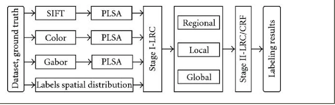
We combine recent several ideas to produce an innovative, accurate, and computationally efficient
two-stage semantic segmentation method. Figure 1 gives an overview of the approach. In the first stage, a rich set of local visual features including SIFT and Gabor textons and robust color histograms is computed, reduced using Probabilistic Latent Semantic Analysis (PLSA) topic models as a form of regularized dimensionality reduction, and combined with learned scene-sensitive spatial layout priors using a Logistic Regression
Classifier (LRC) to produce initial patch-level label probabilities. In the second stage, the spatial coherence of these initial labels is refined by a Conditional Random Field (CRF) or a second stage LRC that combines them with neighboring-patch and global-aggregate contextual features. For accuracy, the CRF is trained with an efficient maximum-margin method that uses cutting plane optimization over subproblems solved with the FastPD graph-cut method. We evaluate our methods on the partially labeled 9- and 21-class MSRC
The paper is organized as follows. Section 2 reviews previous and related work. Sections 3 and 4
describe, respectively, our stage 1 and stage 2 classifiers. Section 5 presents our experimental results, and Section 6 concludes the paper.
2. Previous and Related Work
This section briefly summarizes some relevant recent work on scene segmentation and semantic labeling. He et al. [2] proposed a multiscale CRF that combines local, regional, and global features. Training this model
required inefficient stochastic sampling, but further research [4] resulted in a discriminative image
segmentation framework that integrates bottom-up and top-down cues to infer a considerably wider range of object classes than earlier methods. Kumar and Hebert [5] employed a two-layer CRF to encode long-range and short-range interactions. The boosted random fields of Torralba et al. [6] learn both the graph structure and the feature functions of a CRF. Shotton et al. [7] described a model for discriminating object classes that efficiently incorporates texture, layout, and contextual information. Verbeek and Triggs [8] trained a CRF on partially labeled data and incorporated top-down aggregate features to improve the segmentation. Yang et al. [9] implemented a multiclass, object-based segmentation method using appearance and Bag of
Keypoints features over mean-shift patches. Schroff et al. [10] incorporated globally trained class models into a random forest classifier with multiple features, imposing spatial smoothing via a CRF to improve
accuracy. Toyoda and Hasegawa [11] presented a CRF that models both local and global information, demonstrating high performance on two small fully labeled datasets.
Many articles on image labeling have focused on the use of high-level semantic representations and contextual information. Rabinovich et al. [12] incorporated semantic cues by constructing a CRF over
image regions that encodes co-occurrence preferences for pairs of classes. Verbeek and Triggs [13] combined the advantages of PLSA topic models and Markov Random Field smoothness priors. Cao and Fei-Fei [14]
used Latent Dirichlet Allocation (LDA) topic models to perform region level segmentation and classification, forcing the pixels within a homogeneous region to share the same latent topic. The Latent Topic Random Field [15] learns a novel context representation by capturing patterns of co-occurrence within and between
image features and object labels (i.e., in the joint label/feature space). He and Zemel [16] also explored a hybrid framework that uses partially labeled data by combining a generative topic model for image
appearance with discriminative label prediction. Csurka and Perronhin [17] proposed a simple framework for semantic segmentation: a Fisher kernel derives high-level descriptors for computing class relevance on the patch level, while the context is inferred by classification at the image level. Tu [18] introduced an autocontext scene parsing model that effectively takes contextual information into account: this works well, but training takes several days. Shotton et al. [19] presented a semantic texton forest method that infers the distribution over categories at each pixel and uses an inferred image-level prior to obtaining state-of-the-art performance. The model allows a tradeoff between memory usage and training time.
Many recent methods attempt to capture spatial information by incorporating absolute image location features. In contrast, Galleguillos et al. [20] used qualitative spatial relations (above, below, inside, around) to
capture spatial context, and Gould et al. [21] achieved state-of-the-art results by incorporating
image-dependent relative location features that capture complicated spatial relationships through a two-step classifier.
Like the framework of Verbeek and Triggs [8], our approach is a CRF that exploits global image context as well as local information. However, it differs from [8] in several important ways. Firstly, we include an additional Gabor texton feature channel [22] and an improved color descriptor, and we replace the simple absolute
position features of [8] with more informative spatial layout features based on global scene similarity. Secondly, [8] implicitly uses "naive Bayes" multilinear link functions to generate individual-patch posterior topic
probabilities from its various texton channels. We replace these with nonlinear Logistic Regression Classifiers (LRC), providing more accurate node-level inputs to the CRF. Thirdly, we add region-level cues to our CRF by incorporating neighboring-patch-level features that (among other things) implicitly encode information on the probable relative locations of different object classes. Finally, we improve the accuracy of the CRF by replacing the maximum likelihood training of [8] with a more discriminative and very efficient maximum-margin approach that improves on [23] by using the cutting plane algorithm of [3] over FastPD [24] based subproblem optimization. As the numerical experiments in Section 5 demonstrate, the final
framework provides significant improvements in accuracy, speed, and applicability relative to the state of the art.
3. Stage 1: Patch-Level Classifiers
This section describes our first stage (individual patch level) classifiers. After discussing our visual features we recall the basics of PLSA-based dimensionality reduction, describe how we capture the typical spatial layouts of scene classes, and finally detail the regularized Logistic Regression Classifier (LRC) that ties these
3.1. Local Patch Descriptors
Many visual features have been proposed, encoding properties such as pixel intensities, color, texture, and edges. Here we characterize each patch using three channels of local visual descriptors: vector quantized SIFT [25], color histograms, and Gabor textons. The approach is similar to [8], but we improve their color channel and add a Gabor texton channel. For our color histograms we concatenate the normalized hue and the opponent angle descriptors of Van De Weijer and Schmid [26]. The former are best adapted to scenes with saturated colors, the latter to ones with more muted natural colors. Together they provide a robust description of a wide variety of scenes. For our Gabor descriptors we use the spatially compact and computationally efficient "simple Gabor feature space" of [22]. In each channel the descriptors are vector quantized using k-means dictionaries learned from the training images.
3.2. Low-Dimensional Semantic Representation
"Bag of (local visual) features" (BoF) models, which mimic and were inspired by "bag of words" approaches to natural language processing and information retrieval, have proven very successful for image categorization. In the BoF approach, each image patch is represented by its codeword or words in a vector-quantized
visual feature space, and the whole image is represented by the corresponding histogram over such codewords. For example, if each patch is represented by its SIFT, color, and Gabor descriptors, each
vector quantized using 1000 center k-means codebooks as in [8], the complete image is characterized by its 3 × 1000 element histogram of codeword counts, and indeed each patch can be represented by an analogous binary histogram containing exactly 3 nonzero entries, one for the codeword seen in each feature channel.
Such high-dimensional feature spaces contribute to the overall richness of the model, but they can easily lead to high computational cost and to overfitting in later stages. To counter this, it is useful to find ways of controlling the effective dimensionality of the representation. In both visual and textual applications, latent topic models have proven to be a very effective means for this, in essence offering a form of
probabilistic regularization or dimensionality reduction that focuses attention on the classes most relevant to the particular example in hand.
The most basic latent topic model, Probabilistic Latent Semantic Analysis (PLSA) [27], assumes that there are hidden underlying causes—"topics" or "factors" —that generate codeword values (here quantized
patch descriptors) with some discrete distribution and that the topic of each patch in a given image is generated from an image-specific prior so that the complete probability for the patch is the
discrete mixture
independently over all patches in the image. Given a new image, we must estimate its , and, when learning the whole PLSA model from unlabeled data, we must estimate both for all training images and for all topics. Regularized E-M is used in both cases. Given a patch in image , by Bayes rule, its posterior topic probability is . In this, the naive isolated-patch
posterior is "probabilistically smoothed" to incorporate the influence of the image-wide prior , thus effectively enhancing the probability of the topics that are most useful for describing the image as a whole and reducing the probability of the others.
Latent Dirichlet Allocation (LDA) [28] is a Bayesian form of PLSA that further regularizes by putting a Dirichlet prior on it. This produces a model that is stabler when there are many possible topics and each image is small, unlabeled, and involves only a few of them, but otherwise very similar to PLSA. However, our
application has few topics and comparatively large images, so we prefer PLSA for its much greater
computational efficiency. There are a number of other variants on topic models such as the Harmonium model [29] and Pachinko Allocation [30], which are based, respectively, on undirected graphical models and on directed acyclic graphs of topics. However, we again prefer flat PLSA for its simplicity and efficiency [13].
Quelhas et al. [31] and Bosch et al. [32] showed that unsupervised PLSA can generate a robust low-dimensional representation that captures meaningful aspects of the scene for image classification. Li and Perona [33] proposed two variants of LDA that generate intermediate topic representations for natural scene categories, reporting good categorization performance on a large set of complex scenes.
Rasiwasia Vasconcelos [34] introduced a low-dimensional semantic theme representation that correlates well with human scene understanding, achieving near state-of-the-art performance for scene categorization with low training complexity.
Throughout this paper, we will assume that the latent topics correspond exactly to the predefined semantic classes for scene labeling and that a labeled training set is available. It follows that PLSA training is trivial—we can directly read off both and from the labeled training images—and that the
topic-level probabilities that we output have clear semantics with respect to the scene content.
Finally, note that we describe each patch by separate SIFT, color, and Gabor codewords. It would also be possible to use multimodal PLSA [8] to share a single topic prior between all three modalities,
assuming independent generation of the codeword of each modality from the topic:
(2)
However, for simplicity, we use independent PLSAs (image-specific topic priors) in each modality. This
provides slightly less overall regularization as the three priors are not coupled; however, it does not give rise to any overcounting, particularly as the output probabilities are used only as input features for the stage 1
probabilities forward into the LRC, so the patch feature vector is reduced to dimensions, where is the number of scene classes.
3.3. Spatial Layout of Scene Categories
The previous representation characterizes the patches local appearance, but we can also incorporate cues relating to the typical absolute or relative image positions of the various content classes. For example, "sky" tends to be at the top of the image, "road" at the bottom, and "car" above "road." Moreover, certain
scene categories such as landscapes (water mountains sky) and urban scenes (road cars buildings)
occur frequently and provide useful priors on the spatial layout of the various classes. There are various ways of encoding such information. Absolute image position can be encoded by superimposing a uniform grid on the image and using the index of a patches grid cell as a quantized spatial position feature for it [8]. Conversely, Toyoda and Hasegawa [11] used global color features to capture scene similarity and thus to transfer the spatial label distributions of training images to test images, giving good labeling results for two datasets.
Here we quantify global scene similarity using the Spatial Pyramid Matching (SPM) scheme of [35] over dense-quantized SIFT features, transferring training labels from the nearest training images in a manner similar to [11]. SPM is analogous to the original feature-space pyramid matching scheme of [36], except that it works by subdividing the 2-D image with a quadtree, not the -D feature space (both spaces can also be subdivided simultaneously, but we do not do this here). Given two images and , let the image square be subdivided regularly into cells at levels , and let be the SIFT histogram in cell of level
image . Then, the SPM image similarity metric is
(3)
This can be evaluated by an efficient recursion. Under it, similar (larger ) images are ones that have many similar SIFT histograms at fine levels of their spatial subdivisions, that is, ones that have similar spatial distributions of SIFT codewords.
Given , our spatial prior probability for pixel of image to have label is
(4)
corresponding pixel of image has training label and 0 otherwise. Finally, the spatial prior probability for patch of image to have label is the average of over the pixels of the patch
(5)
Note that in contrast to [11], we use only the nearest neighbors [37] of the image to compute the prior. For small datasets it is possible to use the entire training set, but for larger ones such as MSRC-9 and MSRC-21 it is both more efficient and more accurate to use just the nearest neighbors.
3.4. Regularized Logistic Regression
Linear Logistic Regression is a simple but effective probabilistic classification method that is well suited for use as a stage 1 classifier and that integrates naturally into our overall CRF framework. As individual patches are
classified independently in stage 1, training and evaluation are both very efficient. Given patch feature vector , multivariate Logistic Regression models the probability for patch label to be class as follows:
(6)
where is a matrix of weight vectors with columns , is a vector of class biases,
and is a probability normalization term. Training minimizes the regularized cost function [38]
(7)
where is a regularization parameter and runs over the training examples with features , labels , and normalizations . Lin et al. [38] used a trust region Newton method to minimize this, showing that
this approach is faster than the commonly used quasi-Newton methods and that it yields excellent performance.
4. Stage 2: Enhancing Spatial Coherence
Although their PLSA-based features already incorporate some image-level smoothing based on thetopic probabilities, our first stage classifiers operate essentially at the level of individual patches. The second stage of our method resolves local ambiguity and enhances the spatial contiguity of the labeling by
incorporating additional information from the neighborhood of the patch and from the global image context. We test two kinds of stage 2 classifiers, a Conditional Random Field "LRC/CRF," and a purely feed-forward method "LRC/LRC" based on a second layer of independent-patch-level LRC classifiers that incorporate patch-neighborhood-level features. The second approach is simpler but cruder in the sense that it does not explicitly model interpatch couplings and hence avoids combined global inference across all patches.
Note that both approaches are logically consistent in the sense that the CRF and LRC frameworks allow the inclusion of arbitrary functions of the input features, including ones that incorporate global information (via PLSA), nonlinearities (via the first stage LRCs), and neighbors of the given patch. One of our central insights is that—relative to methods such as [8] that use linear feature probabilities directly as inputs to the CRF
—"cooking" the inputs via a relatively elaborate first-stage classifier offers a degree of nonlinear preprocessing and dimensionality reduction that significantly improves the overall quality of the CRF output.
4.1. Neighborhood and Global Features
To capture some of the correlations between each patch and its neighbours we introduce the neighborhood system shown in Figure 2, the second stage inputs for the given patch being the first stage outputs
(class probabilities) for itself and for all of its neighbors under the selected neighborhood system N1–
N5. Furthermore, we also encode the image-wide context by including a global aggregate feature shared by all patches in the image—the average stage 1 class probabilities aggregated over the whole image, compare [8]. For example, for N5 (5 × 5) neighborhoods in a problem with classes, the vector of inputs would contain
patch-level probabilities, neighboring-patch probabilities, and shared global probabilities. Intuitively,
this local and global contextual information should help the method to produce well-smoothed patch classifications.
Figure 2 The nested set of neighborhoods N1–N5 tested for our patch-neighborhood feature set. N [MediaObjects/13634_2010_Article_2698_IEq67_HTML.
gif] includes all of the neighboring patches numbered
[MediaObjects/13634_2010_Article_2698_IEq68_HTML.
4.2. CRF Model
The above first-stage patch, patch-neighbour, and global-aggregate label probability features can be used directly as inputs to a second layer of individual-patch-level LRC classifiers, giving an overall
feed-forward architecture denoted "LRC/LRC." A more sophisticated alternative is to use them as inputs to an image-wide Conditional Random Field (CRF) model in which the final patch labels interact with one another, providing the scope for more global label smoothing and disambiguation.
whole to individual outputs —and "clique potentials" —scalar couplings linking individual pairs (or more generally multiplets) of outputs in , with listing the directly coupled multiplets:
(8)
The partition function over , , is typically unknown and intractable, but it is constant for any given input image and hence irrelevant for relative probability estimates.
We take the unary potentials to be linear in the stage one outputs:
(9)
Here, are the possible output label values for , the input is the stage 1 output for patch (with feature dimension ), is the set of local displacements to the neighbors of patch , and is the aggregate stage 1 output across the whole image. Typically, the stage 1 output
provides preliminary class labels so , and if we use 5 × 5 neighborhoods . Thus , , and are, respectively, , , and matrices of coefficients to be learned.
Given the results of [8], we test only a simple diagonal Potts model for the clique potentials
(10)
where is 1 if its inputs agree and 0 otherwise and is a scalar coupling parameter to be learned.
4.3. CRF Parameter Estimation
The CRF specifies a conditional distribution for its output labels given its inputs and parameters. We tested both discriminative Maximum Likelihood and Maximum-Margin methods for parameter estimation.
Maximum Likelihood estimation maximizes the conditional log likelihood over the
labeled training examples . Although notionally simple, this requires the evaluation of the partition function , and it is known for its tendency to both converge erratically and overfit. To handle this, we used
In contrast, maximum-margin training does not learn a calibrated and does not require . Instead, it directly forces the CRF energy function to favor the desired labeling over an algorithm-generated set of incorrect ones by a given margin. This can be formulated as a structured output learning problem—a quadratic programming problem with exponentially many constraints corresponding to the possible
incorrect labelings. There are several competing formulations. The Maximum-Margin Markov Network (M3N) [41] incorporates max-margin and output-correlation constraints and uses a dual extra-gradient method to accelerate training. Szummer et al. [23] use structured output support vector machines [42] and maximum-margin network learning [43, 44] but solve the image labelling subproblems efficiently using graphcuts [45]. These methods have proven successful for problems that were difficult to handle using conditional maximum likelihood training.
Our approach is similar to [23] but with two crucial differences. Firstly, we replace the -slack based
training method of [23] with a 1-slack one (i.e., despite the fact that there are exponentially many constraints, a single-slack variable is maintained for all of them). Joachims et al. [3] has demonstrated that 1-slack cutting plane algorithms are equivalent to but substantially faster than -slack ones on a wide range of problems. Here, the speedup can be several orders of magnitude. Secondly, we use FastPD [24] instead of alpha-expansion graphcuts [45] to solve energy optimization (node-labeling) subproblems during both training and testing. FastPD is a state-of-the art algorithm that generalizes prior methods such as alpha expansion, while being an order of magnitude faster in practice [46] and handling more general potentials (including some non-submodular ones) with strong per-instance optimality bounds. For convenience, Algorithm 1 provides pseudocode for the resulting max-margin training algorithm [3].
Algorithm 1: Pseudocode for our 1-slack maximum-margin learning algorithm.
Input: labeled training examples ; regularization parameter ; desired precision .
For any , let
where counts the number of label disagreements
in the image.
Initialize the set of active labelings: .
Update to satisfy the active constraints:
such that for all
.
Use FastPD to find the new MAP labeling for each
training example:
.
Update the set of active labelings:
.
Until: .
4.4. Pixel level Labeling
Our learning and inference methods work at the patch level, so for comparison with other methods we need to interpolate their output to pixel level. The simplest approach sets the class label of a pixel to the label of the patch with the nearest center, but this tends to produce significant blocking artifacts in the output. Instead we tested two postprocessing methods, an MRF based smoother that uses "soft" (probabilistic) patch labels such as those provided by our LRC/LRC method and a local oversegmentation algorithm that uses "hard" labels such as those provided by our LRC/CRF algorithm (whose usual output is a crisp FastPD segmentation, not soft patchwise marginals).
The MRF smoother estimates pixel level posterior class distributions by weighted bilinear interpolation from the four nearest patch-level posteriors, builds a pixel level MRF with these data terms and simple Potts model couplings with parameter 0.7, and runs fast graph-cut optimization on the MRF to obtain the final pixel level labelings. Note that this gives significantly smoother segmentations than running the MRF directly on the patch-level output.
5D feature set that includes the LAB color and the image coordinates of the pixel. The parameters are chosen to provide a significant oversegmentation, with the minimum segment area set to 20 pixels. The method is very fast, taking less than one second per image and generating an average of 424 segments per image on the MSRC-21 dataset.
5. Experimental Results
This section presents our experimental results, comparing our method to recent state-of-the-art approaches on four datasets: the 21-class and 9-class MSRC datasets [1] and the 7-class Sowerby and Corel datasets used in [2].
5.1. Datasets and Experimental Settings
We begin by detailing our datasets and experimental setup. The MSRC-21 dataset contains 591 images hand labeled with 21 classes: building, grass, tree, cow, sheep, sky, airplane, water, face, car, bicycle, flower, sign, bird, book, chair, road, cat, dog, body, and boat. MSRC-9 contains 240 images hand labeled with 9 classes —building, grass, tree, cow, sky, plane, face, car, and bike—and we follow [8] in choosing 120 images for training and 120 for testing. In each case some pixels are unlabeled: following previous works [7], we ignore such pixels during training and evaluation. Each image is covered with overlapping 20 × 20 pixel patches with centers separated by 10 pixels. We report average results over 20 random train-test partitions for MSRC-9 and 5 for MSRC-21.
The 7-class Corel and Sowerby datasets are simpler, with fully labeled ground truth. Sowerby contains 104 urban and rural images with 96 × 64 pixels labeled as sky, vegetation, road marking, road surface, building, street object, or car. Our Corel subset contains 100 natural images with 180 × 120 pixels labeled as rhino/
hippo, polar bear, water, snow, vegetation, ground, or sky. We use 10 × 10 pixel patches with centers spaced by 2 pixels for Sowerby and by 5 pixels for Corel, as in [8]. We follow [2], training on 60 images and testing on the rest, reporting average performances over 10 random training-test partitions.
We quantize the SIFT, color, and Gabor descriptors separately, using by default k-means visual codebooks with 1000 centers each for MSRC-9, Sowerby, and Corel, and with 2000 centers each for MSRC-21. Centers with too few elements are are pruned, and their elements reassigned to the nearest remaining center. For the spatial layout features, we set the number of neighboring training images to 60 for Sowerby and Corel and to 30 for MSRC. For the regional-level features in the second stage, we use 5 × 5 patch neighborhoods
5.2. Quantitative Results
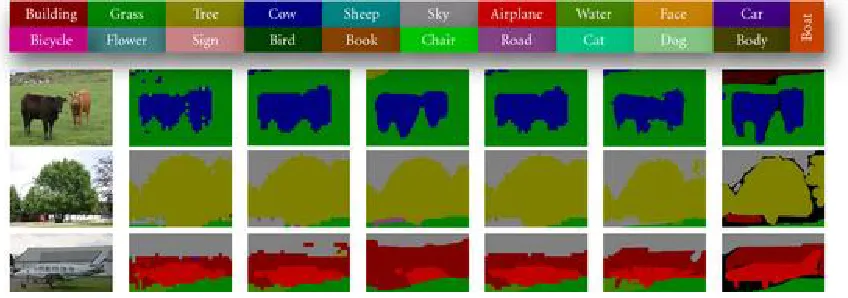
Figure 3 shows some representative and some less-good segmentation results for various methods on MSRC-21, and Table 1 gives the pixel level accuracies of our algorithms (top line) and various others (bottom line) on MSRC-21. Relative to the stage 1 LRC classifier, including the stage 2 CRF improves the results by about 3% for nearest-patch labeling and 4% for oversegmentation labeling.
Table 1 Mean pixel level accuracies for various algorithms on MSRC-21.
Algorithm LRC/NP* LRC/LRC/NP* LRC/LRC/MRF* LRC/CRF/NP* LRC/CRF/OS*
Accuracy (%) 72.7 75.4 76.7 75.9 76.8
Algorithm TextonBoost [7] PLSA-MRF [13] Mean shift [9] STF-ILP [19] AC (ACP) [18] RLP-CRF [21]*
Accuracy (%) 72.2 73.5 75.1 72 74.5 (77.7) 76.5
*These methods give results averaged over five random train/test partitions. The others give results for a single partition.
Figure 3 Sample segmentation results for the MSRC-21 dataset. The first 8 rows show
Table 2 Pixel level confusion percentages for our LRC/CRF/OS method on the MSRC-21 dataset. The mean pixel level accuracy is 76.9%.
Inferred class
Building Grass Tree Cow Sheep Sky Aeroplane Water Face Car Bike Flower Sign Bird Book Chair Road Cat Dog Body Boat True class
Building 62.8 1.7 10.5 0.1 0 3.2 0.2 2.1 2.6 0.4 3.5 0 0 0.1 2.3 1.4 7.6 0 0 1.2 0.3 Grass 0.9 94.5 1.4 0.1 0.3 0.1 0.1 0.6 0 0 0 0.3 0 0 0 0 1.6 0 0 0.2 0
Tree 2.2 6.7 82.1 0 0 2.6 0.2 0 0 0 0 4.2 0 0 0 0 0.6 0 0 1.3 0.1
Cow 0 21.4 0.3 70.1 4.0 0 0 0.8 0 0 0 0.1 0 0 0 0 0.5 0.4 0.1 2.2 0
Sheep 0 19.8 0 0.1 79.7 0 0 0 0 0 0.2 0 0 0 0 0 0.2 0 0 0 0
Sky 1.7 0.1 0.5 0 0 92.2 0.1 0 0 0 0 0 0 5.1 0 0 0.3 0 0 0 0
Aeroplane 23.6 10.4 0.8 0.8 0 5.0 56.4 0 0 0 0 0 0 0 0 0 3.0 0 0 0 0
Water 3.3 3.4 6.3 0 0 2.8 0.2 66.5 0 0 0 0 0 2.8 0.9 0 13.4 0 0 0.4 0.1 Face 4.2 0.4 4.0 0 0 1.1 0 0.3 72.4 0 0 0.3 0 0 3.9 0.1 0.1 0 6.9 6.2 0
Car 12.1 0 2.0 0 0 0.1 0 0.0 0 62.6 0 0 0 0.6 0 0.2 15.0 5.8 0 0 1.6
Bike 5.7 0.3 0.8 0 0 0 0 0 0 0.4 70.1 0 0 0 0 9.0 13.6 0 0 0 0 00
Flower 0 0.4 1.9 0 0 0 0 0 0 0 0 97.6 0 0 0 0 0 0 0 0.1 0
Sign 40.4 0.1 1.4 0 0 1.6 0 0 0 0 0 4.2 42.7 0 9.0 0 0.3 0.1 0 0.3 1.0 Bird 4.6 11.5 3.5 0.9 0.8 3.2 3.0 5.9 0 3.5 0 6.5 0 43.5 0 7.8 4.3 0 0 0 0
Book 3.1 0.1 0 0 0 0.2 0 0 0.2 0 0 0 0 0 96.1 0 0.1 0 0 0.2 0
Chair 0.4 19.3 7.3 4.4 0 0 0 3.6 0 0 2.1 0 0.9 1.2 2.4 53.5 4.8 0 0 0 0 Road 4.0 2.0 1.1 0 0 1.7 0.0 8.6 0.1 0.7 1.0 0 0 0 0 0.1 80.2 0 0 0.4 0
Cat 3.0 0.1 0.3 0 0 0.6 0 5.4 0 0 0.4 0 0 4.0 0 0 12.1 74.1 0 0 0
Dog 2.4 5.1 3.0 7.4 0 0.5 0 16.1 7.2 0 4.0 0 0 1.7 0.4 0 10.7 3.8 35.1 2.7 0 Body 7.1 6.5 10.7 0.7 0 0.4 0 6.3 4.1 0 0 1.0 0 0.4 5.7 1.9 3.8 0 4 45.8 1.4 Boat 29.8 0.1 0 0 0 2.2 0.5 28.8 0 1.5 5.7 0 0 1.8 0 0 9.6 0 0 2.2 17.9
A comparison of the output of the LRC/LRC and LRC/CRF methods shows that the CRF one is more consistent and that its errors are visually more reasonable, even though the absolute patch-labeling accuracies differ by only 0.02–0.07%. Figure 3 illustrates that for the sign and bird images, LRC/CRF (column (e)) provides more correct labels than LRC/LRC (column (c)). Similarly, the pixel level refinements based on
A notable aspect of our methods is their speed of training and testing, which makes them scalable to
larger problems. The reported average training and testing times per image for various algorithms on MSRC-21 are shown in Table 3 (None of these figures include time spent on feature extraction and codebook formation and use. Our results are on a 3.4 GHz PC with 3.8 Gb of memory.). The use of FastPD for inference in our CRFs reduces testing times to less than 0.02 seconds. Regarding postprocessing, our MRF smoother takes 2– 4 seconds per image, while our oversegmenter takes 1-2 seconds.
Table 3 Reported training and testing times for various algorithms on MSRC-21.
Method Training time Test time
TextonBoost [7] 2 days 30 sec/image
PLSA-MRF [13] 1 hour 2 sec/image
STF-ILP [19] 2 hours <0.125 sec/image
AC(ACP) [18] a few days 30–70 sec/image
Our LRC/LRC 7-8 min <0.03 sec/image
Our LRC/CRF 30–35 min <0.02 sec/image
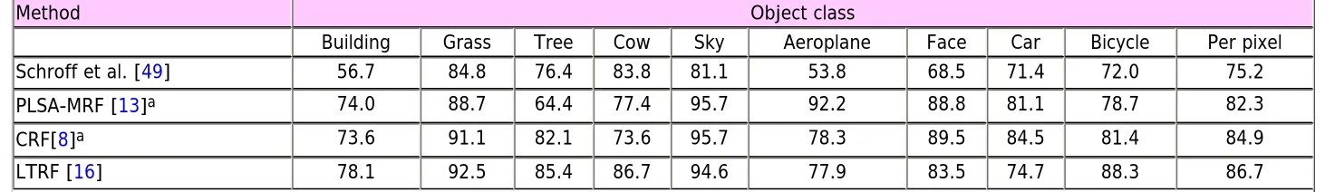
Various results for the MSRC-9 dataset are shown in Table 4. Our LRC/CRF classifier improves the state of the art [21] by 0.1%. For completeness we also report the lowest and highest accuracies over 20 random partitions for this method.
Table 4 Pixel level labeling accuracies (%) for various algorithms on MSRC-9.
Method Object class
Building Grass Tree Cow Sky Aeroplane Face Car Bicycle Per pixel
Schroff et al. [49] 56.7 84.8 76.4 83.8 81.1 53.8 68.5 71.4 72.0 75.2
PLSA-MRF [13]a 74.0 88.7 64.4 77.4 95.7 92.2 88.8 81.1 78.7 82.3
CRF[8]a 73.6 91.1 82.1 73.6 95.7 78.3 89.5 84.5 81.4 84.9
RF-CRF [10] — — — — — — — — — 87.2
RLP-CRF [21]b — — — — — — — — — 88.5
Our LRC/CRF-avea 82.4 93.9 85.2 81.8 93.8 76.0 92.6 90.2 88.5 88.6
Our LRC/CRF-min 79.5 90.8 87.9 77.7 90.7 72.6 91.2 82.6 95.2 86.6
Our LRC/CRF-max 86.6 94.7 87.7 87.7 91.8 83.5 98.8 92.4 86.3 90.7
aFor these methods the results are averages over 20 random train-test partitions. bFor this method the results are averages over 5 random train-test partitions.
Figure 4 shows some illustrative labelings obtained on Sowerby and Corel by single-stage LRC, LRC/LRC, and LRC/CRF. Visually, the max-margin CRF appears to give the best results in most cases. The single-stage LRC produces many isolated label errors as each patch is predicted independently. Table 5 summarizes various results obtained on Sowerby and Corel. For comparison, over 10 random partitions, the accuracies of our LRC/CRF method range from 86.8% to 91.2% on Sowerby and from 71.5% to 81.3% on Corel. Note that, for Corel, we did not use the preprocessor of [7, 21].
Table 5 Pixel level labeling accuracies for various algorithms on Sowerby and Corel.
Method Performance
Sowerby Corel
Accuracy Training time Test time Accuracy Training time Test time
Shotton et al. [7] 88.6% 5 h 10 s 74.6% 12 h 30 s
He et al. [2] 89.5% Gibbs Gibbs 80.0% Gibbs Gibbs
Verbeek and Triggs [8] 87.4% 20 min 5 s 74.6% 15 min 3 s
Toyoda and Hasegawa [11] 90.0% — — 83.0% — —
Gould et al. [21]* 87.5% — — 77.3% — —
Our LRC/CRF* 89.1% 8 min <0.02 s 77.0% 7 min <0.02 s
*For these methods the results are averages over 10 random train-test partitions. The others use a single partition.
5.3. Discussion
We now examine several aspects of our approach in more detail.
5.3.1. Feature Histograms versus PLSA Posterior
Features versus Patch-Level LRC
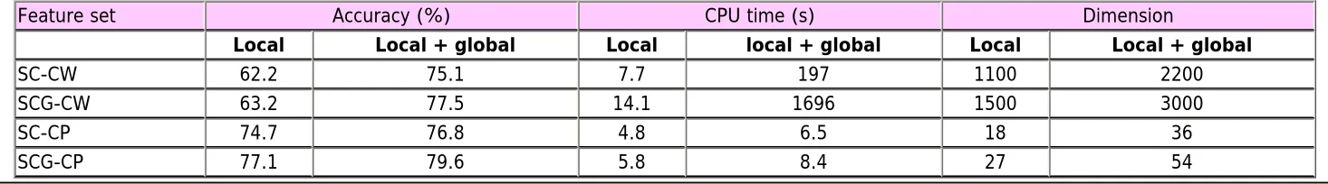
respectively, quantized using 1000, 100 and 400 center k-means codebooks, and testing both local-only and local + global aggregate feature configurations. Table 6 reports the results, using patch-level LRC as the final classifier. We see that, relative to codewords, the class-posterior representation significantly increases the accuracy while greatly reducing both the dimensionality and the run time. Given the comparatively poor results for codewords using local-only features, it seems advisable to include either global aggregate features or PLSA smoothing—both work well, while combining them produces only a modest further improvement.
Table 6 Patch-level accuracies of linear PLSA and mPLSA classifiers and nonlinear LRC classifiers, for various posterior-probability feature sets on MSRC-9.
Descriptor SIFT Color Gabor SIFT + Color SIFT + Gabor Color + Gabor SIFT + Color + Gabor
Classifier PLSA PLSA PLSA LRC mPLSA LRC mPLSA LRC mPLSA LRC mPLSA
Accuracy (%) 60.1 59.1 52.8 74.7 73.8 65.5 56.4 73.6 70.3 77.1 71.9
CPU time (s) 0.8 0.3 0.5 4.8 41.9 5.0 51.4 4.9 22.6 5.8 59.5
Table 7 compares the nonlinear Logistic Regression Classifier (LRC) with the linear multimodal PLSA (mPLSA) classifier used in [13] and with linear single-mode PLSA, again for various combinations of
posterior-probability features on the MSRC-9 dataset. LRC is uniformly more accurate than mPLSA and also much faster, with the full SIFT + Color + Gabor LRC giving the best overall accuracy as expected. In
contrast, mPLSA sometimes becomes less accurate as additional channels are added (e.g., when adding Gabor to SIFT or to SIFT + Color).
Table 7 Patch-level performances of CRF learning by the likelihood maximization (ML) and margin maximization (MM) methods, using only SIFT and color descriptors on MSRC-9 class data.
Method ML/SP_LBP MM/ICM MM/MP_LBP MM/TRWS MM/GC MM/FastPD
EF-1 EF-2 EF-1 EF-2 EF-1 EF-2 EF-1 EF-2 EF-1 EF-2* EF-1 EF-2
Accuracy (%) 76.3 78.9 75.4 77.9 76.8 79.3 77.0 79.5 76.9 – 76.9 79.6
CPU time (s) 6954.5 7288.4 307.4 205.4 5041.9 3290.2 2471.4 2122.9 140.8 – 100.2 150.9 *GC failed here because SVMStruct does not enforce hard constraints on the weights and requested a
5.3.2. Max-Margin versus Max-Likelihood CRF Training
Table 8 compares various Maximum-Margin and Maximum Likelihood training methods for the CRF classifier, on MSRC-9 for posterior probability features over a 1000 center SIFT codebook and a 100 center Color codebook. The learning methods tested are as follows.
Table 8 Patch-level accuracies for the stage 1 LRC on MSRC-9 for various feature sets: SIFT (S), Color (C) and Gabor (G) descriptors represented by codewords (CW) or PLSA class probabilities (CP), using only local features, or local ones + global aggregates.
Feature set Accuracy (%) CPU time (s) Dimension
Local Local + global Local local + global Local Local + global
SC-CW 62.2 75.1 7.7 197 1100 2200
SCG-CW 63.2 77.5 14.1 1696 1500 3000
SC-CP 74.7 76.8 4.8 6.5 18 36
SCG-CP 77.1 79.6 5.8 8.4 27 54
For ML training we use Stochastic Gradient Descent (SGD) optimization, with sum-product loopy belief propagation (SP_LBP) to approximate the partition function and infer the labels. For efficiency, the SGD gradient gain needs to be set as high as possible while maintaining stability [40]: we set it to 10−4 and run at most 40 iterations; the best result appearing in the 35th iteration in this experiment.
For Max-Margin training we tested the 1-slack optimizer described above with several subproblem solvers (label inference methods) [50]: Iterated Conditional Modes (ICM), Max-Product Loopy Belief
Propagation (MP_LBP), Tree-Reweighted Message Passing (TRWS), alpha expansion Graph Cuts (GC), and FastPD.
For each of these methods we tested two energy functions, both with simple scalar 4-neighbor Potts couplings, but with different forms of unary potential over the PLSA-based class posteriors and
for the label of node given the corresponding feature codeword . In the first model (EF-1)
the unary terms take the diagonal form , where the are
As the table shows, the Max-Margin approaches dominate the Max-Likelihood ones in both accuracy and run time. Of the Max-Margin subproblem solvers tested, TRWS, GC, and FastPD are all about equally accurate, but GC sometimes fails to converge, and TRWS is slow, leaving FastPD as the method of choice. The matrix-based energy formulation is consistently 2-3% more accurate than the scalar one with little increase in training time.
5.3.3. The Benefits of Neighborhood Information and Context
Figure 5 shows how including stage 1 spatial layout features, stage 2 global context, and various different stage 2 neighborhood sizes influences the results of LRC/LRC and LRC/CRF on the MSRC-9 and MSRC-21 datasets. The methods tested are the following:(i) N0-I: LRC over independent PLSA posterior probabilities for SIFT, color, and Gabor;
(ii) N0-II: N0-I with spatial layout features added to the LRC;
(iii) N0: N0-II with the inclusion of global aggregate features as well as local ones in stage 2;
(iv) Nk, : N0 with the inclusion of the features from the given th degree local neighborhood in stage 2- c.f. Figure 2.
CRF consistently outperforms LRC/LRC, but the differences become negligible when the spatial layout and global aggregate features are included.
Note that for N0-I, the accuracy of LRC/CRF on MSRC-9 reaches 82.1%. This is 5% better than the 77.1% reported in Table 7. Both methods use the SIFT, Color, and Gabor descriptors, but here we used a combination of hue and opponent angle as the color descriptor and tested with a 1000 center codebook not a 100 center one.
6. Conclusion
Segmenting images into semantically meaningful regions is an important task in image analysis. Our efficient two-stage algorithm incorporates various local visual appearance features, example-based spatial layout priors, and neighborhood-level and global context cues, producing semantic image segmentations that are
significantly more accurate than those achieved by the best previous patch-based methods and on a par with those of state-of-the-art pixel-based ones [18, 21] despite being much faster.
The first stage of the algorithm uses a PLSA topic model to provide regularized dimensionality reduction of its vector quantized input features, feeding the resultant posterior topic probabilities into individual-patch-level Logistic Regression Classifiers (LRCs). The second stage incorporates additional patch-neighborhood and global aggregate features, using either a further layer of LRCs or a Conditional Random Field to produce the final output labeling. The method is fast and scalable to large problems, in part owing to the use of high-quality existing software including LIBLINEAR [48] for LRC training and SVMStruct [3] and FastPD [24] for CRF training.
Future Work
The current method is limited in the sense that it works at a single scale using patches of constant size. This will presumably limit its ability to handle classes whose image scale varies significantly and whose
appearance varies with scale. It would be useful to develop a multiscale variant of the approach, perhaps using different topic models at each scale.
BodyRef
FileRef : BodyRef/PDF/13634_2010_Article_2698.pdf
The authors would like to thank Professor T. Joachims of Cornell University for his help with SVMStruct. The research was supported in part by the Chinese National Natural Sciences Foundation Grants 40801183 and 60890074 and by European Union IST project 027978 CLASS.
Acknowledgments
References
1. Criminisi AMicrosoft research Cambridge object recognition image database
(version 1.0 and 2.0), 2004,
http://research.microsoft.com/en-us/projects/objectclassrecognition/
2. He X, Zemel RS, Carreira-Perpiñán MÁ:
Multiscale conditional random
fields for image labeling.
Proceedings of the 2004 IEEE Computer Society
Conference on Computer Vision and Pattern Recognition (CVPR '04), July 2004
II695-II702.
3. Joachims T, Finley T, Yu CNJ:
Cutting-plane training of structural SVMs.
Machine Learning
2009,
76
(1):27-59.
4. He X, Zemel RS, Ray D:
Learning and incorporating top-down cues in
image segmentation.
Proceedings of the 9th European Conference Computer
Vision, 2006
1:
338-351.
5. Kumar S, Hebert M:
A hierarchical field framework for unified
context-based classification.
Proceedings of the 10th IEEE International Conference on
Computer Vision (ICCV '05), 2005
1284-1291.
6. Torralba A, Murphy KP, Freeman WT:
Contextual models for object
detection using boosted random fields.
Advances in Neural Information
Processing Systems
2005,
17:
1401-1408.
7. Shotton J, Winn J, Rother C, Criminisi A:
TextonBoost: joint appearance,
shape and context modeling for multi-class object recognition and
segmentation.
Proceedings of the 9th European Conference on Computer Vision
(ECCV '06), 2006, Lecture Notes in Computer Science
3951:
1-15.
8. Verbeek J, Triggs B:
Scene segmentation with CRF learned from partially
labeled images.
In
Advances in Neural Information Processing Systems
. MIT
Press, Cambridge, Mass, USA; 2008:1553-1560.
11. Toyoda T, Hasegawa O:
Random field model for integration of local
information and global information.
IEEE Transactions on Pattern Analysis
and Machine Intelligence
2008,
30
(8):1483-1489.
12. Rabinovich A, Vedaldi A, Galleguillos C, Wiewiora E, Belongie S:
Objects
in context.
Proceedings of the IEEE 11th International Conference on Computer
Vision (ICCV 07), October 2007
13. Verbeek J, Triggs B:
Region classification with Markov field aspect
models.
Proceedings of the IEEE Computer Society Conference on Computer
Vision and Pattern Recognition (CVPR '07), June 2007
14. Cao L, Fei-Fei LI:
Spatially coherent latent topic model for concurrent
segmentation and classification of objects and scenes.
Proceedings of the IEEE
11th International Conference on Computer Vision (ICCV '07), October 2007
15. He X, Zemel RS:
Latent topic random fields: learning using a taxonomy
of labels.
Proceedings of the 26th IEEE Conference on Computer Vision and
Pattern Recognition (CVPR 08), June 2008
16. He X, Zemel RS:
Learning hybrid models for image annotation with
partially labeled data.
Advances in Neural Information Processing Systems
2008.
17. Csurka G, Perronnin F:
A simple high performance approach to semantic
segmentation.
Proceedings of the British Machine Vision Conference, 2008
18. Tu Z:
Auto-context and its application to high-level vision tasks.
Proceedings of the 26th IEEE Conference on Computer Vision and Pattern
Recognition (CVPR '08), June 2008
19. Shotton J, Johnson M, Cipolla R:
Semantic texton forests for image
categorization and segmentation.
Proceedings of the 26th IEEE Conference on
Computer Vision and Pattern Recognition (CVPR '08), June 2008
20. Galleguillos C, Rabinovich A, Belongie S:
Object categorization using
co-occurrence, location and appearance.
Proceedings of the 26th IEEE Conference
on Computer Vision and Pattern Recognition (CVPR '08), 2008
21. Gould S, Rodgers J, Cohen D, Elidan G, Koller D:
Multi-class segmentation
with relative location prior.
International Journal of Computer Vision
2008,
80
(3):300-316. 10.1007/s11263-008-0140-x
22. Kyrki V, Kämäräinen JK, Kälviäinen H:
Simple Gabor feature space for
invariant object recognition.
Pattern Recognition Letters
2004,
25
(3):311-318.
10.1016/j.patrec.2003.10.008
23. Szummer M, Kohli P, Hoiem D:
Learning CRF using graph cuts.
24. Komodakis N, Tziritas G:
Approximate labeling via graph cuts based on
linear programming.
IEEE Transactions on Pattern Analysis and Machine
Intelligence
2007,
29
(8):1436-1453.
25. Lowe DG:
Distinctive image features from scale-invariant keypoints.
International Journal of Computer Vision
2004,
60
(2):91-110.
26. Van De Weijer J, Schmid C:
Coloring local feature extraction.
Proceedings
of the 9th European Conference Computer Vision, 2006, Lecture Notes in
Computer Science
3952:
334-348.
27. Hofmann T:
Unsupervised learning by probabilistic latent semantic
analysis.
Machine Learning
2001,
42
(1-2):177-196.
28. Blei DM, Ng AY, Jordan MI:
Latent Dirichlet allocation.
Journal of
Machine Learning Research
2003,
3
(4-5):993-1022.
29. Xing E, Yan R, Hauptmann A:
Mining associated text and images with
dual-wing harmoniums.
In
Proceedings of the 21th Annual Conference on
Uncertainty in Artificial Intelligence, 2005
. AUAI press;
30. Li W, McCallum A:
Pachinko allocation: DAG-structured mixture
models of topic correlations.
Proceedings of the 23rd International Conference
on Machine Learning (ICML '06), 2006
577-584.
31. Quelhas P, Monay F, Odobez JM, Gatica-Perez D, Tuytelaars T, Van Gool L:
Modeling scenes with local descriptors and latent aspects.
Proceedings 10th
IEEE International Conference on Computer Vision (ICCV '05), 2005
883-890.
32. Bosch A, Zisserman A, Muñoz X:
Scene classification via pLSA.
Proceedings of the 9th European Conference Computer Vision, 2006, Lecture
Notes in Computer Science
3954:
517-530.
33. Li FF, Perona P:
A bayesian hierarchical model for learning natural scene
categories.
Proceedings of the IEEE Computer Society Conference on Computer
Vision and Pattern Recognition (CVPR '05), 2005
524-531.
34. Rasiwasia N, Vasconcelos N:
Scene classification with low-dimensional
semantic spaces and weak supervision.
Proceedings of the 26th IEEE
Conference on Computer Vision and Pattern Recognition (CVPR '08), 2008
35. Lazebnik S, Schmid C, Ponce J:
Beyond bags of features: spatial pyramid
matching for recognizing natural scene categories.
Proceedings of the IEEE
Computer Society Conference on Computer Vision and Pattern Recognition
(CVPR '06), June 2006
2169-2178.
38. Lin CJ, Weng RC, Keerthi SS:
Trust region Newton methods for
large-scale logistic regression.
Proceedings of the 24th International Conference on
Machine Learning (ICML '07), June 2007
561-568.
39. Lafferty J, McCallum A, Pereira F:
Conditional random fields:
probabilistic models for segmenting and labeling sequence data.
Proceedings
of the 18th International Conference Machine Learning, 2001
282-289.
40. Vishwanathan SVN, Schraudolph NN, Schmidt MW, Murphy KP:
Accelerated training of conditional random fields with stochastic gradient
methods.
Proceedings of the 23rd International Conference on Machine
Learning (ICML '06), June 2006
969-976.
41. Taskar B, Lacoste-Julien S, Jordan MI:
Structured prediction, dual
extragradient and bregman projections.
Journal of Machine Learning
Research
2006,
7:
1627-1653.
42. Tsochantaridis I, Joachims T, Hofmann T, Altun Y:
Large margin methods
for structured and interdependent output variables.
Journal of Machine
Learning Research
2005.,
6:
43. Anguelov D, Taskar B, Chatalbashev V, Koller D, Gupta D, Heitz G, Ng A:
Discriminative learning of Markov Random fields for segmentation of 3D
scan data.
Proceedings of the IEEE Computer Society Conference on Computer
Vision and Pattern Recognition (CVPR '05), June 2005
169-176.
44. Taskar B, Chatalbashev V, Koller D, Guestrin C:
Learning structured
prediction models: a large margin approach.
Proceedings of the 22nd
International Conference on Machine Learning (ICML '05 ), August 2005
896-903.
45. Boykov Y, Veksler O, Zabih R:
Fast approximate energy minimization via
graph cuts.
IEEE Transactions on Pattern Analysis and Machine Intelligence
2001,
23
(11):1222-1239. 10.1109/34.969114
46. Komodakis N, Tziritas G, Paragios N:
Performance vs computational
efficiency for optimizing single and dynamic MRFs: setting the state of the
art with primal-dual strategies.
Computer Vision and Image Understanding
2008,
112
(1):14-29. 10.1016/j.cviu.2008.06.007
47. Comaniciu D, Meer P:
Mean shift: a robust approach toward feature
space analysis.
IEEE Transactions on Pattern Analysis and Machine Intelligence
2002,
24
(5):603-619. 10.1109/34.1000236
48. Fan RE, Chang KW, Hsieh CJ, Wang XR, Lin CJ:
LIBLINEAR: a library
for large linear classification.
Journal of Machine Learning Research
2008,
9:
49. Schroff F, Criminisi A, Zisserman A:
Single-histogram class models for
image segmentation.
Proceedings of the Indian Conference Computer Vision,
Graphics and Image Processing, 2006
![Table 2 presents the overall confusion matrix on MSRC-21 for our LRC/CRF method with oversegmentation-based refinement, using the data partition of [7]](https://thumb-us.123doks.com/thumbv2/123dok_us/1149405.1144302/17.792.41.474.26.469/table-presents-overall-confusion-matrix-oversegmentation-refinement-partition.webp)