Real World Instrumentation with Python.pdf

(1)

(2)

(3)

(4)

Real World Instrumentation

with Python

J. M. Hughes

(5)

Real World Instrumentation with Python by J. M. Hughes

Published by O’Reilly Media, Inc., 1005 Gravenstein Highway North, Sebastopol, CA 95472.

O’Reilly books may be purchased for educational, business, or sales promotional use. Online editions are also available for most titles (http://my.safaribooksonline.com). For more information, contact our corporate/institutional sales department: 800-998-9938 or [email protected].

Editor: Julie Steele

Production Editor: Adam Zaremba Copyeditor: Rachel Head Proofreader: Sada Preisch

Indexer: John Bickelhaupt Cover Designer: Karen Montgomery Interior Designer: David Futato

Illustrator: J. M. Hughes and Robert Romano

Printing History:

November 2010: First Edition.

Nutshell Handbook, the Nutshell Handbook logo, and the O’Reilly logo are registered trademarks of O’Reilly Media, Inc. Real World Instrumentation with Python, the image of a hooded crow, and related trade dress are trademarks of O’Reilly Media, Inc.

Many of the designations used by manufacturers and sellers to distinguish their products are claimed as trademarks. Where those designations appear in this book, and O’Reilly Media, Inc., was aware of a trademark claim, the designations have been printed in caps or initial caps.

While every precaution has been taken in the preparation of this book, the publisher and author assume no responsibility for errors or omissions, or for damages resulting from the use of the information con-tained herein.

TM

This book uses RepKover™, a durable and flexible lay-flat binding.

ISBN: 978-0-596-80956-0

(6)

3. The Python Programming Language . . . 59

Installing Python 60

The Python Programming Language 61

The Python Command Line 61

Command-Line Options and Environment 63

Objects in Python 64

Data Types in Python 65

Expressions 77

Operators 78

Statements 84

Strings 91

Program Organization 96

Importing Modules 106

Loading and Running a Python Program 108

Basic Input and Output 110

Hints and Tips 115

Python Development Tools 117

Editors and IDEs 117

Debuggers 120

Summary 120

4. The C Programming Language . . . 123

Installing C 123

Developing Software in C 124

A Simple C Program 125

Preprocessor Directives 128

Standard Data Types 132

User-Defined Types 133

Operators 134

Expressions 143

Statements 143

Arrays and Pointers 150

Structures 153

Functions 156

(8)

Building C Programs 159

C Language Wrap-Up 163

C Development Tools 163

Summary 164

5. Python Extensions . . . 167

Creating Python Extensions in C 168

Python’s C Extension API 169

Extension Source Module Organization 169

Python API Types and Functions 171

The Method Table 172

Method Flags 172

Passing Data 174

Using the Python C Extension API 175

Generic Discrete I/O API 175

Generic Wrapper Example 178

Calling the Extension 181

Python’s ctypes Foreign Function Library 184

Loading External DLLs with ctypes 184

Basic Data Types in ctypes 186

Using ctypes 187

Summary 188

6. Hardware: Tools and Supplies . . . 189

The Essentials 189

Hand Tools 190

Digital Multimeter 192

Soldering Tools 195

Nice-to-Have Tools 197

Advanced Tools 198

The Oscilloscope 198

Logic Analyzers 199

Test Equipment Caveats 202

Supplies 203

New Versus Used 204

Summary 204

7. Physical Interfaces . . . 207

Connectors 208

DB-Type Connectors 208

(9)

USB Connectors 210

Circular Connectors 212

Terminal Blocks 213

Wiring 215

Connector Failures 218

Serial Interfaces 218

RS-232/EIA-232 219

RS-485/EIA-485 225

USB 231

Windows Virtual Serial Ports 235

GPIB/IEEE-488 237

GPIB/IEEE-488 Signals 238

GPIB Connections 239

GPIB via USB 239

PC Bus Interface Hardware 241

Pros and Cons of Bus-Based Interfaces 242

Data Acquisition Cards 244

GPIB Interface Cards 244

Old Doesn’t Mean Bad 245

Summary 246

8. Getting Started . . . 249

Defining the Project 250

Requirements-Driven Design 251

Stating the Need 252

Project Objectives 253

Requirements 253

Why Requirements Matter 255

Well-Formed Requirements 256

The Big Picture 257

Requirement Types 257

Use Cases 258

Traceability 261

Capturing Requirements 264

Designing the Software 265

The Software Design Description 265

Graphics in the SDD 266

Pseudocode 270

Divide and Conquer 270

Handling Errors and Faults 272

Functional Testing 273

(10)

Test Cases 274

Testing Error Handling 277

Regression Testing 278

Tracking Progress 279

Implementation 279

Coding Styles 280

Organizing Your Code 281

Code Reviews 282

Unit Testing 286

Connecting to the Hardware 295

Documenting Your Software 296

Version Control 299

Defect Tracking 299

User Documentation 300

Summary 300

9. Control System Concepts . . . 303

Basic Control Systems Theory 304

Linear Control Systems 305

Nonlinear Control Systems 306

Sequential Control Systems 308

Terminology and Symbols 309

Control System Block Diagrams 310

Transfer Functions 312

Time and Frequency 313

Control System Types 318

Open-Loop Control 319

Closed-Loop Control 319

Nonlinear Control: Bang-Bang Controllers 326

Sequential Control Systems 330

Proportional, PI, and PID Controls 332

Hybrid Control Systems 340

Implementing Control Systems in Python 340

Linear Proportional Controller 340

Bang-Bang Controller 341

Simple PID Controller 342

Summary 346

10. Building and Using Simulators . . . 349

What Is Simulation? 350

Low Fidelity or High Fidelity 351

(11)

Simulating Errors and Faults 352

Using Python to Create a Simulator 356

Package and Module Organization 356

Data I/O Simulator 357

AC Power Controller Simulator 371

Serial Terminal Emulators 380

Using Terminal Emulator Scripts 381

Displaying Simulation Data 383

gnuplot 383

Using gnuplot 385

Plotting Simulator Data with gnuplot 388

Creating Your Own Simulators 391

Justifying a Simulator 392

The Simulation Scope 392

Time and Effort 393

Summary 393

11. Instrumentation Data I/O . . . 395

Data I/O Interface Software 395

Interface Formats and Protocols 396

Python Interface Support Packages 406

Alternatives for Windows 412

Using Bus-Based Hardware I/O Devices with Linux 412

Data I/O: Acquiring and Writing Data 414

Basic Data I/O 414

Blocking Versus Nonblocking Calls 421

Data I/O Methods 423

Handling Data I/O Errors 426

Handling Inconsistent Data 431

Summary 435

12. Reading and Writing Data Files . . . 437

ASCII Data Files 438

The Original ASCII Character Set 439

Python’s ASCII Character-Handling Methods 439

Reading and Writing ASCII Flat Files 442

Configuration Data 449

Module AutoConvert.py—Automatic String Conversion 451

Module FileUtils.py—ASCII Data File I/O Utilities 454

Binary Data Files 463

(12)

Handling Binary Data in Python 466

Image Data 476

Summary 485

13. User Interfaces . . . 487

Text-Based Interfaces 487

The Console 487

ANSI Display Control Techniques 500

Python and curses 515

To Curse or Not to Curse, Is That the Question? 523

Graphical User Interfaces 524

Some GUI Background and Concepts 524

Using a GUI with Python 526

TkInter 529

wxPython 535

Summary 543

14. Real World Examples . . . 547

Serial Interfaces 547

Simple DMM Data Capture 548

Serial Interface Discrete and Analog Data I/O Devices 553

Serial Interfaces and Speed Considerations 559

USB Example: The LabJack U3 560

LabJack Connections 560

Installing a LabJack Device 562

LabJack and Python 562

Summary 570

A. Free and Open Source Software Resources . . . 573

B. Instrument Sources . . . 579

Index . . . 583

(13)

(14)

Preface

This is a book about automated instrumentation, and the automated control systems used with automated instrumentation. We will look at how to use the Python pro-gramming language to quickly and easily implement automated instrumentation and control systems.

Automated instrumentation can be found in a wide variety of settings, ranging from research laboratories to industrial plants. As soon as people realized that collecting data over time was a useful endeavor, they also realized that they needed some way to capture and record the data. Of course, one could sit with a clock and a pad of paper, staring at thermometers, dials, and gauges, and write down numbers or other information every few minutes or so, but that gets tedious rather quickly. It’s much easier—and more reliable—if the process can be automated. Fortunately, technology has advanced significantly since the days of handwritten logbooks and clockwork-driven strip chart recorders.

Nowadays, one can purchase inexpensive instrumentation for a wide variety of physical phenomena and use a computer to capture the data. Once a computer is connected to instrumentation, the possibilities for data collection, analysis, and control begin to expand in all directions, with the only real limitations being the ability to implement the necessary software and the implementer’s creativity.

The primary objective of this book is to show you how to create software that you can use to get a capable and user-friendly instrumentation or control application up and running with a minimum of hassle. To this end, we will work through the steps nec-essary to create applications that incorporate low-level interfaces to the real world via various types of input/output hardware. We will also examine some proven methods for creating programs that are robust and reliable. Special attention will be paid to designing the algorithms necessary to acquire and process the data. Finally, we will see how to display the results to a user and accept command inputs. It is my desire that you will find ideas here that you might take away and creatively apply to meet your own needs in a wide variety of settings.

(15)

Who Is This Book For?

This is a hands-on text intended for people who want or need to implement instru-mentation systems, also known as data acquisition and control systems. You might be a researcher, a software developer, a student, a project lead, an engineer, or a hobbyist. The application might be an automated electronics test system, an analysis process in a laboratory, or some other type of automated instrumentation.

One of the objectives with the software in this book is that it be as platform-independent as possible. I am going to assume that you are comfortable with at least the Windows platform, and Windows XP in particular. With Linux I’ll be referring to the Ubuntu distribution, but the discussion should apply to any recent Linux distribution and I will assume that you know how to use either the csh or bash command-line shells. Since this is a book about interfacing to the real world via physical hardware, some electronics are involved, but I am not going to assume that you have an extensive back-ground in electrical engineering. Chapter 2 contains an overview of the basics of elec-tronics theory as it relates to instrumentation, for those who might benefit from it. It turns out that it really doesn’t take a deep level of electronics knowledge to successfully interface a computer with the physical world. But, as with anything else involving technology, it never hurts to know as much as possible, just on the off chance that things don’t quite work out as expected the first time.

Regardless of the type of work you do, or where you do it, the main thing I am assuming that we have in common is a need to capture some data, and perhaps to generate control signals, and to do so through some kind of computer interface. Most importantly, we need the instrumentation and control software we create to be accurate, reliable, and relatively painless to implement.

The Programming Languages

The primary programming language we will use is Python, with a bit of C thrown in. Throughout the book, I will assume that you have some programming experience and are familiar with either Python or C (ideally, both). If that is not the case, experience with Perl or Tcl/Tk or analysis tools such as MatLab or IDL is also a reasonable starting point.

(16)

Why Python?

Python is an interpreted language developed by Guido van Rossum in the late 1980s. Because of its interpreted nature, there is no compilation step to deal with, and the user can create and execute programs directly from Python’s command line. The language itself is also easy to learn and comprehend, so long as one initially avoids the more advanced features (generators, introspection, list comprehension, and such). Thus, Python offers the dual benefits of rapid prototyping and ease of comprehension, which in turn allows for the quick creation of sophisticated tools for a diverse range of instrumentation applications, without the development burdens and learning curve normally associated with conventional compiled languages or a vendor-specific pro-gramming environment.

Python is highly portable, and it is available for almost every modern computing plat-form. So long as a project sticks to using commonly available interface methods, an application written initially on a PC running Windows will most likely work without change on a machine running Linux. The odds are good that the application will also run on a Sun Solaris machine or an Apple OS X system, although these systems are not specifically covered in this text. It is only when Python is used in conjunction with platform-specific extensions or drivers that it loses its portability, so in these cases I will offer alternatives for both Windows and Linux wherever feasible.

The text includes example code snippets, block diagrams and flow charts to illustrate key points, and some complete examples utilizing readily available and low-cost inter-face hardware.

The Systems

The types of instrumentation systems we will examine might be utilized for laboratory research, or they might be used in industrial settings. An instrumentation system might be used in an electronics lab, in a wind tunnel, or to collect meteorological data. The systems may be as simple as a temperature data logger or as complex as a thermal vacuum chamber control system.

Generally, just about anything that can be interfaced to a PC is a potential candidate for the techniques described in this book. There are, of course, some devices with closed proprietary interfaces, but I will not address those, nor will I delve into complex data collection and process control scenarios such as oil refineries, nuclear power plants, or robotic spacecraft. Systems in those domains are usually best served with sophisticated and complex custom control hardware, and equally sophisticated and complex soft-ware. I will focus instead on those instruments, devices, and systems that can be easily programmed using any of a number of common interface methods.

(17)

Methodology

Using a step-by-step approach and real-world examples, we will examine the processes necessary to define the instrumentation application, select the appropriate interfaces and hardware, and create the low-level extension modules needed (if any) to interface Python with instrumentation hardware. We will also investigate the use of TkInter, wxPython, and curses for graphical and text-based user interfaces.

The book includes sections describing what is involved in writing an extension for Python in order to encapsulate a hardware vendor’s DLL; how to communicate with USB-based I/O devices; and how to use industry-standard interfaces such as RS-232, RS-485, and GPIB, along with a survey of what types of hardware one might expect to find using these interfaces. It also provides references to readily available open source tools and libraries to reduce, as much as possible, the amount of time spent imple-menting functionality from scratch.

How This Book Is Organized

This book is organized into 14 chapters and 2 appendixes. The first 12 chapters set the stage for the implementation examples described in Chapter 14. Chapters 1 through

6 introduce basic concepts that the advanced reader may elect to skip over. Here’s a closer look at what you’ll find in each chapter:

Chapter 1, Introduction to Instrumentation

Chapter 1 provides an overview of what instrumentation is, how control systems work, and how these concepts are used in the real world. The examples covered include automatic outdoor lights, test instrumentation in an electronics engineer-ing environment, control of a thermal chamber in a laboratory, and batch chemical processing.

Chapter 2, Essential Electronics

Because this is a hands-on book, we will need to know something about the phys-ical hardware we want to interface to and have at least a general idea of how it works. This chapter starts off with an introduction to the basic concepts of elec-tricity and electronics. It then explores the functional building blocks for data ac-quisition and control, including discrete digital interfaces, analog interfaces, and counters and timers. Lastly, it reviews the basic concepts behind serial and parallel interfaces. If you are already familiar with electric circuit theory and devices, you could skip this chapter. However, I would recommend that you still at least skim through the material, on the off chance that there might be something unique here that you can make use of later.

Chapter 3, The Python Programming Language

(18)

book. This chapter also provides a brief overview of the tools available to make life easier for the person doing the programming, and where to go about finding them.

Chapter 4, The C Programming Language

Here, the C programming language is introduced in a high-level overview. The objective is to provide enough information to enable you to understand the exam-ples in this book, without delving into the arcane details. Fortunately, C is a rela-tively simple language, and the information in this chapter should be sufficient to get you started on creating your own extensions for Python.

Chapter 5, Python Extensions

This chapter describes how a Python extension is created, and what extensions are typically used for. Examples are provided, both in this chapter and in later chapters, for you to use as templates for your own efforts.

Chapter 6, Hardware: Tools and Supplies

Although is it possible that one could implement an instrumentation system and never touch a soldering iron, there is a high probability that some screwdrivers, wire cutters, and a digital multimeter (DMM) will come in handy. In this chapter I provide a list of what I would consider to be a basic toolkit for doing instrumen-tation work. It isn’t much and could all easily fit in a small box on a shelf some-where. However, there could very well come a time when you really need to see what’s going on in your system. To this end, I’ve included a discussion of the two pieces of test equipment that can help you eliminate the guesswork and quickly get to the root of an interface or control problem: the oscilloscope and the logic analyzer. This chapter also covers what types of instruments are available and pro-vides some suggestions for deciding between buying new equipment or picking up something used.

Chapter 7, Physical Interfaces

Chapter 7 examines the types of interfaces one is most likely to encounter when attempting to interface Python to data acquisition or control instrumentation. RS-232 and RS-485, the two most commonly encountered types of serial interfaces, are examined from an instrument interface perspective. This chapter also covers the basics of USB and GPIB/IEEE-488 interfaces, along with a discussion of where one might expect to encounter them. Finally, we turn our attention to I/O hardware designed to be plugged into the bus of a PC, typically PCI-type circuit boards, and what one can typically expect in terms of API support from the hardware vendor.

Chapter 8, Getting Started

This chapter contains a description of a proven approach to software development. It is included here because, when implementing an instrument system in any lan-guage, it is essential to plan and define what is to be implemented, and then to test the result against the expectations captured in a set of requirements. By extending the reach of Python into the real world, we open the door for the uncertainties and vagueness of the real world to wander back in and impact—sometimes severely— the instrumentation software.

(19)

Chapter 9, Control System Concepts

A book on real-world data acquisition and control would be incomplete without a discussion of control systems and the theory behind them. Chapter 9 expands on the concepts introduced in Chapter 1 with detailed examinations of common control system concepts and models, including topics such as feedback, “bang-bang” controllers, and Proportional-Integral-Derivative (PID) controls. It also pro-vides an introduction to basic control system analysis and propro-vides some guidelines for choosing an appropriate model. Lastly, we’ll look at how the mathematics of control systems translates into actual Python code.

Chapter 10, Building and Using Simulators

Chapter 10 examines simulators and how they can be leveraged to speed up the development process, provide a safe environment in which to test out ideas, and provide some invaluable (and otherwise unattainable) insights into the behavior of not only the instrumentation software, but also the device or system being si-mulated. Whether because the instrumentation hardware just isn’t available yet or because the target system is too valuable to risk damaging, a simulation can be a quick and easy way to get the software running, test it, and have a high degree of confidence that it will work correctly in the real world.

Chapter 11, Instrumentation Data I/O

In this chapter we’ll look at how to use the interfaces that were introduced in

Chapter 7 to move data between the real world and your applications. We’ll start with a discussion of interface formats and protocols in order to define the basic concepts we will need for the upcoming software examples, and then we’ll take a quick tour of some packages that are available for interface support in Python with the pySerial, pyParallel, and PyVISA packages. Lastly, I’ll show you some techni-ques to read and write instrumentation data. We’ll take a look at blocking versus nonblocking I/O, asynchronous input and output events, and how to manage po-tential data I/O errors to help make your applications more robust.

Chapter 12, Reading and Writing Data Files

Chapter 12 examines some of the implementation considerations and techniques for saving instrumentation data in a variety of file formats, from plain ASCII and CSV files to binary files and databases. We’ll also examine Python’s configuration data file capabilities, and see how easy it is to store and retrieve configuration parameters using Python’s library methods.

Chapter 13, User Interfaces

(20)

Chapter 14, Real World Examples

In Chapter 14 we look at several different types of devices used for data acquisition and control applications. This chapter starts with an example of capturing the continuous data output from a digital multimeter. We then examine a common type of data acquisition device that uses a serial interface for command and data exchanges. Lastly, we wrap up with a detailed look at a data I/O device with a USB interface and its associated API DLL provided by the vendor. The selected devices illustrate key concepts shared by almost all instrumentation components, and the examples draw on earlier chapters to show how the theory is put into practice. Two appendixes provide additional useful information:

Appendix A, Free and Open Source Software Resources Appendix B, Instrument Sources

Conventions Used in This Book

The following typographical conventions are used in this book:

Italic

Indicates new terms, URLs, email addresses, filenames, and file extensions Constant width

Used for program listings, as well as within paragraphs to refer to Python modules and to program elements such as variable or function names, data types, state-ments, and keywords

Constant width bold

Shows commands or other text that should be typed literally by the user Constant width italic

Shows text that should be replaced with user-supplied values or values determined by context

This icon signifies a tip, suggestion, or general note.

This icon indicates a warning or caution.

(21)

Using Code Examples

This book is here to help you get your job done. In general, you may use the code in this book in your programs and documentation. You do not need to contact us for permission unless you’re reproducing a significant portion of the code. For example, writing a program that uses several chunks of code from this book does not require permission. Selling or distributing a CD-ROM of examples from O’Reilly books does require permission. Answering a question by citing this book and quoting example code does not require permission. Incorporating a significant amount of example code from this book into your product’s documentation does require permission.

We appreciate, but do not require, attribution. An attribution usually includes the title, author, publisher, and ISBN. For example: “Real World Instrumentation with Python by J. M. Hughes. Copyright 2011 John M. Hughes, 978-0-596-80956-0.”

If you feel your use of code examples falls outside fair use or the permission given above, feel free to contact us at [email protected].

Safari® Books Online

Safari Books Online is an on-demand digital library that lets you easily search over 7,500 technology and creative reference books and videos to find the answers you need quickly.

With a subscription, you can read any page and watch any video from our library online. Read books on your cell phone and mobile devices. Access new titles before they are available for print, and get exclusive access to manuscripts in development and post feedback for the authors. Copy and paste code samples, organize your favorites, down-load chapters, bookmark key sections, create notes, print out pages, and benefit from tons of other time-saving features.

O’Reilly Media has uploaded this book to the Safari Books Online service. To have full digital access to this book and others on similar topics from O’Reilly and other pub-lishers, sign up for free at http://my.safaribooksonline.com.

How to Contact Us

Please address comments and questions concerning this book to the publisher: O’Reilly Media, Inc.

1005 Gravenstein Highway North Sebastopol, CA 95472

800-998-9938 (in the United States or Canada) 707-829-0515 (international or local)

(22)

We have a web page for this book, where we list errata, examples, and any additional information. You can access this page at:

http://www.oreilly.com/catalog/9780596809560/

To comment or ask technical questions about this book, send email to:

[email protected]

For more information about our books, conferences, Resource Centers, and the O’Reilly Network, see our website at:

http://www.oreilly.com

Acknowledgments

I would like to acknowledge some of the people who helped make this book possible: my wife, Carol, and daughter, Seren, for their patience and understanding when I nee-ded to disappear into my office for extennee-ded periods; my friend and co-worker Michael North-Morris for his perpetual optimism; my acquisition editor, Julie Steele, for her willingness to take a chance and extend to me the opportunity to write for O’Reilly; Rachel Head, the diligent copyeditor, for catching my abuses of the English language; and all of the helpful and friendly staff at O’Reilly.

I would also like to thank the folks at LabJack Corporation for providing me with real hardware to work with and graciously offering their time and support to help make sure I got it working correctly. Thanks also to Janet Smith of Agilent for providing me with high-quality photographs of some of their products.

—John Hughes Tucson, Arizona, 2010

(23)

(24)

CHAPTER 1

Introduction to Instrumentation

However far modern science and technics have fallen short of their inherent possibilities, they have taught mankind at least one lesson: Nothing is impossible.

—Lewis Mumford, Technics and Civilization, 1934

Instrumentation is a big word, with a broad and rich set of meanings. Like most words with multiple interpretations, the exact meaning is largely a function of the context in which it is used, and who is using it.

Instrumentation can be defined as the application of instruments, in the form of systems or devices, to accomplish some specific objective in terms of measurement or control, or both. Some examples of physical measurements employed in instrumentation sys-tems are listed in Table 1-1.

Table 1-1. Examples of physical measurements

Acceleration Mass Capacitance Position Chemical properties Pressure Conductivity Radiation Current Resistance Flow rate Temperature Frequency Velocity Inductance Viscosity Luminosity Voltage

As natural human language is an imprecise communications medium, contextually sensitive and rife with multiple possible meanings, the preceding definition still covers a lot of territory. To a process engineer, it might mean pressure sensors, heater elements, solenoid-controlled valves, and conveyors. A research scientist might think of lasers,

(25)

optical power sensors, servo-driven X-Y microscope stages, and event counters. An electrical engineer might define instrumentation as digital voltmeters, oscilloscopes, frequency counters, spectrum analyzers, and power supplies.

Generally speaking, whatever can be measured can also be controlled, although some things are more difficult to control than others (at least with our current technology). When a measured input value is used to generate a control output for a system, often referred to as the plant, the input may need to be modified, or transformed, in some way in order to match the operating parameters of the system. This might entail am-plification, conversion from current to voltage, time delays, filtering, or some other type of transformation.

In this book, we will examine how to utilize computer-based instrumentation using readily available low-cost devices, along with the Python programming language (pri-marily), to perform various tasks in data acquisition and control. Using a high-level approach, this chapter introduces some of the basic concepts we will be working with throughout the rest of the book. It also shows some simple instrumentation examples. If you are not familiar with some of the concepts introduced in this chapter, don’t be overly concerned about it. We will discuss them in more detail later. The primary ob-jective here is to lay some groundwork and introduce some basic terminology.

Data Acquisition

From a computer’s viewpoint, all data is composed of digital values, and all digital values are represented by voltage or current levels in the computer’s internal circuitry. In the world outside of the computer, physical actions or phenomena that cannot be represented directly as digital values must be translated into either voltage or current, and then translated into a digital form. The ability to convert real-world data into a digital form is a vast improvement over how things were done in the past.

In the days of steam and brass, one might have monitored the pressure within a boiler or a pipe by means of a mechanical gauge. In order to capture data from the gauge, someone would have to write down the readings at certain times in a logbook or on a sheet of paper. Nowadays, we would use a transducer to convert the physical phe-nomenon of pressure into a voltage level that would then be digitized and acquired by a computer.

(26)

When referring to digital data, we mean binary values encoded in the form of bits that a computer can work with directly. Binary digital data is said to be discrete, and a single bit has only two possible values: 1 or 0, on or off, true or false. Digital data is typically said to have a size, which refers to the number of bits that make up a single unit of data.

Figure 1-1 shows digital data ranging from a single bit to a 16-bit word. The size of the data, in bits, determines the maximum value it can represent. For example, an 8-bit byte has 256 possible unique values (if using only positive values).

Figure 1-1. Binary data sizes

For inputs from things such as sensor switches, the size might be just a single bit. In other cases, such as when measuring analog data like pressure or temperature, the input might be converted into binary data values of 8, 10, 12, 16, or more bits in size. The number of available bits determines the range of numeric values that can be represented. Although it’s not shown in Figure 1-1, binary data can represent negative values as well as positive values, and there is a standard format for handling floating-point values as well.

Analog data, on the other hand, is continuously variable and may take on any value within a range of valid values. For example, consider the set of all possible floating-point values in the range between 0 and 1. One might find numbers like 0.01, 0.834, 0.59904041123, or 0.00000048, and anything in between. The name analog data is derived from the fact that the data is an analog of a continuously variable physical phenomenon.

(27)

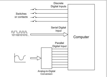
Figure 1-2 shows the various types of inputs that may be found in a computer-based data acquisition system. Switches are the equivalents of single binary digits (bits). A serial communications interface may be a single wire carrying a stream of bits end-to-end, where each set of 8 bits represents a single alphanumeric character, or perhaps a binary value. Analog input signals, in the form of a voltage or a current, are converted into digital values using a device called an analog-to-digital converter (ADC). We will take a close look at these devices—and their counterparts, digital-to-analog converters (DACs)—in Chapter 2.

Figure 1-2. Digital and analog data inputs

Control Output

(28)

open-loop and closed-loop, depending on whether or not they employ the concept of feedback.

Another common type of control system, the sequential control, utilizes time as its primary control input. In a sequential system, events occur at specific times relative to a primary event, and each event is typically discrete. In other words, a sequential event is either on or off, active or inactive. A computer is, by its very nature, a form of sequential controller, and sequential controls can usually be modeled using state ma-chines. We’ll look at state diagrams in Chapter 8.

We will encounter all three types of control systems in this book. Chapter 9 goes into the theory behind them in more detail, but for now, a high-level overview will suffice to set the stage.

Open-Loop Control

In an open-loop scheme, there is no feedback between the output and the control input of the system. In other words, the system has no way to determine if the control output actually had the desired effect. However, this doesn’t prevent it from being useful. The accuracy of an open-loop control system depends on the accuracy of its components and how well the system models what it is controlling. Figure 1-3 shows a simple block diagram of an open-loop control system. The block labeled “Controlled Device” might be an electric motor, a lamp, a fan, or a valve. While it might appear that there isn’t much going on here, open-loop controls can actually entail a high degree of complexity and they are fairly common.

Figure 1-3. Open-loop control

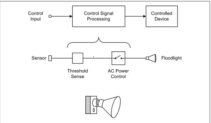
Even though an open-loop control system is “blind,” in a sense, it can still incorporate time into its design. An automatic light switch is one possible real-world example. A greatly simplified diagram of such a device is shown in Figure 1-4.

(29)

Figure 1-4. Open-loop control example

These popular devices contain a sensor (typically infrared) that will activate a floodlight if something appears in the field of view of the sensor. There is no feedback to ensure that the lights actually come on (at least, not in the typical units for residential use), nor can the sensor easily distinguish between a burglar and a large housecat.

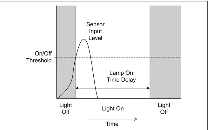
An automatic light does, however, have a built-in time delay to hold the light on for a period of time after the sensor’s input threshold has been crossed; otherwise, it would just turn on and then immediately turn back off again when the sensor input dropped back below the threshold. This is shown in the diagram in Figure 1-5. If there were no time delay to hold the lamp on, a large housecat hopping up and down in front of the sensor would cause the light to flash on and off repeatedly. This would probably annoy the neighbors (then again, automatic lights with excessive time delays can annoy the neighbors as well).

Closed-Loop Control

(30)

Figure 1-5. Open-loop control with time delay

Figure 1-6. Closed-loop control

Notice that the control input and the feedback signal are summed with opposing signs at the circle symbol in Figure 1-6, which is called a “summing junction” or “summing node.” The output is called the control error. This is because the key to a closed-loop control is the response of the controlled device to the control signal generated by the block labeled “Control Signal Processing.” The control error is input to the control signal processing block, and the system will attempt to drive its control output into the controlled device to whatever extent is needed or possible in order to make the control error zero. Those readers who are familiar with operational amplifier (op amp) circuits will recognize this immediately: it’s the same principle that op amp circuits are based on.

(31)

As one might suspect, there is more going on here than the system diagram in Fig-ure 1-6 shows. Both the control and feedback processing blocks may have some degree of amplification (gain) incorporated into their design. They may also include attenua-tion, filters, or limit thresholds. Gain levels are selected based on the applicaattenua-tion, and responses may even be nonlinear if necessary.

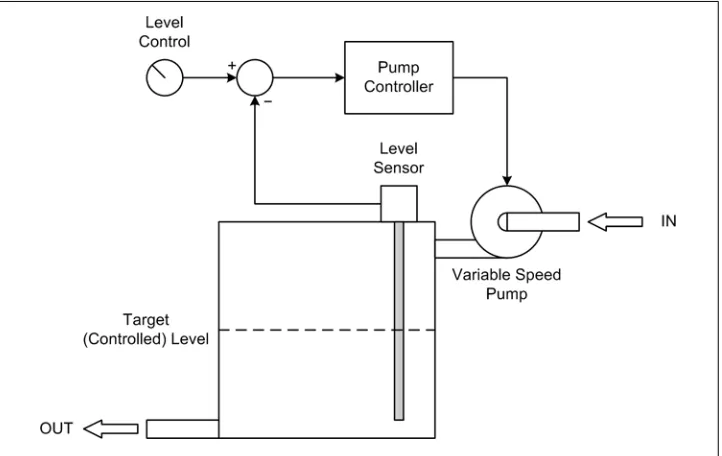
Here’s a somewhat more interesting closed-loop control example. Let’s assume that we want to maintain a constant fluid level in a storage tank while its contents are removed at varying rates. At some times the drain rate may be quite high, while at other times it may be very low or even zero. Figure 1-7 shows the setup and its associated control loop.

Figure 1-7. Closed-loop fluid level control

(32)

Sequential Control

Sequential controls are a very common form of control system and are straightforward to implement. Automated packaging systems, such as those used to form cereal boxes or fill plastic bags with animal feed, are typically timed sequential controls that perform specific actions using electrical or pneumatic actuators. Other sequential controls might employ some type of sensing to change sequences as necessary, or to sense a fault condition and halt the system.

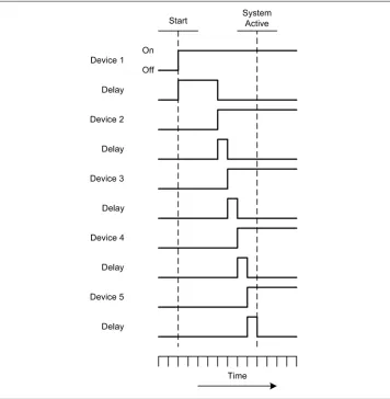
Figure 1-8 shows the timing diagram for a sequential AC power controller with five devices. In this example, a delay after each device is powered on allows it to stabilize and respond to a query to verify that it is functioning correctly. In a system such as this, each device would typically have three possible states: On, Off, and Fail. In addition to commanding the devices on or off in a timed sequence, the controller would also check each device to verify that it powered up correctly. Should a device fail, the con-troller would either halt the sequence or begin an automatic shutdown by disabling the devices already enabled, in reverse order.

Applications Overview

Let’s take a quick tour of some real-world examples of computer-based instrumentation applications. Please bear in mind that these examples are intended to show what one can do with automated instrumentation, not as specific, detailed examples of how to do something. In later chapters we will get into the specifics of interfaces, control pro-tocols, and software algorithms.

Electronics Test Instrumentation

In an electronics laboratory, or even a well-equipped hobbyist’s workshop, it wouldn’t be unusual to encounter oscilloscopes, logic analyzers, frequency meters, signal gen-erators, and other such devices. While these are useful devices in their own right, when incorporated into an automated system they can become even more useful.

In order to use a piece of test equipment in an automated setup, there must be some type of control or acquisition interface available. Many modern instruments incorpo-rate USB, Ethernet, GPIB, RS-232, or a combination of these (these interfaces are ex-amined in Chapters 7 and 11). In some cases, they are standard features; in other cases, the functionality must be ordered as a separate option when the instrument is purchased.

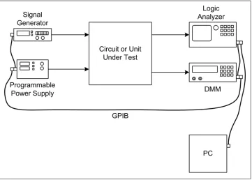
Figure 1-9 shows a simple arrangement for driving a device (the unit under test, or UUT) with a signal while controlling its DC power source, and acquiring measurement data in the form of logic analyzer traces and digital multimeter (DMM) readings.

(33)

The simple setup shown in Figure 1-9 has one instrument connected as a primary stimulus input to the UUT: namely, the signal generator. The signal it generates has a programmable shape (waveform) and rate (frequency). The signal level (amplitude) can also be controlled by the PC. There are two instruments connected to outputs from the UUT to capture digital logic signals (the logic analyzer) and one or more voltages (the DMM). A programmable power supply rounds out the instruments by providing a computer-controlled source of power to the UUT.

In this example, the various instruments are connected to the PC using a General Pur-pose Interface Bus (GPIB, also referred to as IEEE-488). There are various GPIB inter-face components available, ranging from plug-in PCI cards to external USB-to-GPIB adapters. Later in this book, we’ll examine some of these and look at various ways to write software for them in order to control instruments and collect data.

(34)

But what does it do? What Figure 1-9 shows could well be a performance characteri-zation setup. If the UUT generates a pattern of digital signals in response to an input from the signal generator, this test arrangement will capture that behavior. It will also capture how the UUT’s behavior might change as the output from the programmable power supply is changed, or how some internal voltage might change as the frequency of the input from the signal generator changes. All of this data can be displayed on the PC’s monitor and captured to disk for storage and possible analysis at a later time.

Figure 1-9. Test instrumentation example

Laboratory Instrumentation

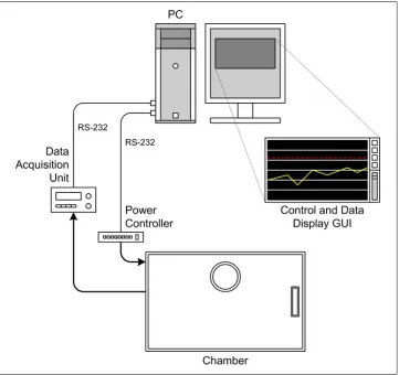
A research laboratory might contain pH meters, temperature sensors, precision ovens, tunable lasers, and vacuum pumps (for starters). Figure 1-10 shows an example of an instrumentation system for controlling an environmental chamber.

For our purposes, it’s not really important what the chamber is used for (it could be used for microbe cultures, or perhaps for epoxy curing). What is important are the instruments connected to it and how they, in turn, are interfaced to the computer. Whereas in the previous example the instrument interface was implemented using GPIB, here we have plain old vanilla serial connections in the form of RS-232 interfaces.

(35)

The data acquisition instrument is responsible for sensing and converting analog signals such as temperature, and perhaps humidity. It might also monitor the electrical status of any heaters or coolers attached to the chamber. The power controller instrument is responsible for any heaters, coolers, cryogenic valves, or other controlled functions in the chamber.

Figure 1-10. Laboratory instrumentation example

(36)

If implemented as a bang-bang controller, a type of on-off non-linear controller that we will look at in detail later on, there won’t be any need to vary the amount of power applied to the heaters or the cooling system. It operates much like the thermostat in a house. The instrumentation can utilize the rather slow RS-232 interfaces because there is no need to run the controller with a small time constant (i.e, a fast acquisition rate).

Process Control

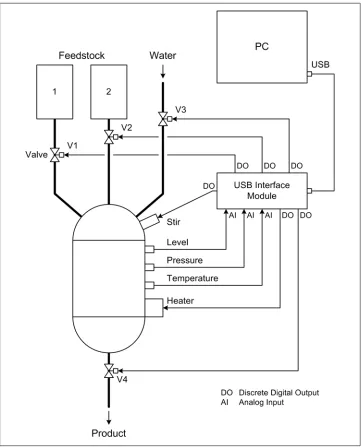
The diagram in Figure 1-11 is a representation of a simple automated process control system. This system might be intended for producing artificial maple syrup, or it could be some other kind of controlled chemical reaction to produce a specific output prod-uct. Note that the diagram is somewhat nonstandard, mainly because its intent is to illustrate without getting wrapped up in the details of standardized process control symbology.

In Figure 1-11, we see yet another type of interface—the USB interface module. These are common and relatively inexpensive. You can even buy one as a kit if you feel inclined to build it yourself. Many provide a set of discrete inputs and outputs, some analog inputs with 10- or 12-bit conversion, and perhaps even some analog outputs or a pulse-width modulation (PWM) channel or two.

There are four valves in the diagram shown in Figure 1-11, labeled V1 through V4, each of which is connected to one of the discrete outputs from the USB interface module. A heater is also connected to a discrete output. Note that the diagram does not show any circuitry that might be necessary to convert the 5-volt discrete signal from the USB controller into something with enough current and/or voltage to drive the valves or the heater. We’ll examine how to drive external devices that utilize high currents or high voltages (or both) in Chapter 2. Three analog inputs are used to acquire liquid level, temperature, and pressure data from sensors.

As with the previous example, this probably would not be a high-speed system. It would most likely perform just fine if the sensors were read and the controls (valves and heater) updated every 1 to 5 seconds.

Summary

The domain of instrumentation applications is both broad and deep, and there is no way that a single chapter like this could possibly capture more than just a glimpse of what it is and what is possible. Some of the terms and concepts may have seemed new and strange, but they will be covered again in later chapters. The main goal here was to give you some exposure to the basic concepts. We’ll fill in the details as we go along.

(37)

(38)

CHAPTER 2

Essential Electronics

Electricity is actually made up of extremely tiny particles called electrons that you cannot see with the naked eye unless you have been drinking.

—Dave Barry, American humorist

Although this is a book primarily about instrumentation software, we must also con-sider what the software is interacting with in the physical world—in other words, the hardware aspects of instrumentation. This chapter is intended to provide a general high-level overview of electricity and basic electronics from an instrumentation per-spective, without delving too deeply into the theory and physics behind it all.

Electronics is a deep and vast field of study. Out of a desire to avoid turning this book into a reference work on the subject, some topics are lightly glossed over here, or not even covered at all. If you’re already familiar with electronics at more than just an Ohm’s law level, feel free to skip over this chapter and forge ahead, but if you’re not quite certain what Ohm’s law is, or about the difference between a current source and a current sink, what the term “waveform” means, or how digital and analog input and output differ from one another, this chapter is for you.

We’ll start off with a general description of electric charge and current, and then present some of the symbols used in schematic diagrams. Next, we’ll take a look at very basic DC and AC circuits, followed by a discussion of the types of input and output found in instrumentation systems from an electrical viewpoint. In later chapters, new con-cepts will be introduced and explained as necessary. We’ll conclude this chapter with a list of references for those who would like to learn more about electronics.

Electrical Charge

For most people, the term “electricity” typically refers to the stuff that one finds in the wires strung along poles beside the street, in a wall outlet, inside a computer, or at the terminals of a battery. But what is it, exactly?

(39)

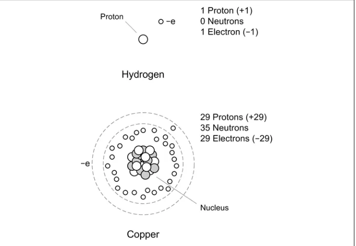
All matter is composed of atoms. Each atom has a nucleus at its core with a net positive charge, and one or more electrons are bound to it, each of which has a negative charge (although one might hear that the electrons “orbit” the nucleus, this is not entirely accurate in the classical sense of an orbit, like, say that of the Earth around the Sun; I would refer you to a modern chemistry or physics text for a better definition than I’m prepared to deliver here). The nucleus of an atom may have one or more protons, each with a positive charge. Most atoms also have a collection of neutrons, which have mass but no charge (one might think of them as ballast for the atom’s nucleus). A typical atom on a typical day in a typical chunk of matter will have a net charge of zero, because there are as many electrons, each with a unit charge of −1, as there are protons in the nucleus, each of which carries a unit charge of +1. Figure 2-1 shows schematic repre-sentations of a hydrogen atom and a copper atom.

Figure 2-1. Atom organization

Some atoms have electrons that are tightly bound, whereas others can lose or gain electrons rather easily. Here’s a simplistic description as to why that is.

(40)

valence electron. Because this electron isn’t very tightly bound, copper doesn’t put up too much of a fuss about passing it around. In other words, copper is a good conductor. An element such as sulfur, on the other hand, does not willingly give up any electrons. Sulfur is rated as one of the least conductive elements, so it’s a good insulator. Silver tops the list as the most conductive element, which explains why it’s considered useful in electronics.

This should be a sufficient model for our purposes, so we won’t pry any further into the inner secrets of atomic structure. What we’re really interested in here is what hap-pens when atoms do pass electrons around, and why they would do that to begin with.

Electric Current

There are two fundamental phenomena involved in electricity: electric charge and elec-tric current. Elecelec-tric charge is a basic characteristic of matter and is the result of some-thing having too many electrons (negative charge) or too few electrons (positive charge), with regard to what it would otherwise need to be electrically neutral.

A basic characteristic of electric charges is that charges of the same kind repel one another, and opposite charges attract. This is why electrons and protons are bound together in an atom, although they can’t directly combine with each other because of some other fundamental characteristics of atomic particles. The important thing to remember is that a negative charge will repel electrons, and a positive charge will attract them.

Electric charge, in and of itself, is interesting but not particularly useful from an elec-tronics perspective. For our purposes, it’s only when charges are moving that really interesting things begin to happen. Electric current, or current flow, is the flow of elec-trons through a circuit of some kind. It is also what happens when the static charge you build up walking across a carpet on a cold, dry day is transferred to a doorknob: in effect, the current flows from a high potential (you) to a lower potential (the door-knob), much like water flows down a waterfall. The otherwise uninteresting static charge suddenly becomes very interesting (at least, it gets your attention).

Current flow arises when the atoms that make up the conductors and components of electrical circuits transfer electrons from one to another. Electrons move toward things that are positive, so if one has a small lightbulb attached to a battery with some wires (sometimes known as a flashlight), the electrons move out of the negative terminal of the battery, through the lightbulb, and return back into the positive terminal. Along the way, they cause the filament in the lamp to get white-hot and glow. One way to visualize the current flow is shown in Figure 2-2, where we see a simplified diagram of some copper atoms in a wire. When an electron is introduced into one end of the wire, it causes the first atom to become negatively charged. It now has too many electrons. Assuming that we have a continuous source of electrons with a net negative charge, the new electron cannot exit the way it came in, so it moves to the next available neutral

(41)

atom. This atom is now negative and has a surplus electron. In order to become neutral again (the preferred state of an atom) it passes its extra electron to the next (neutral) atom, and so on, until an electron appears at the other end of the wire.

Another way to think about current is shown in Figure 2-3. In this case, we have a tube (a conductor) filled end-to-end with marbles (electrons).

When we push a marble into one end of the tube, a marble falls out the opposite end. The net number of marbles in the tube remains the same. Note that the electrons put into one end of a conductor are not necessarily the ones that come out the other end, as one can see from Figures 2-2 and 2-3.

Figure 2-2. Electron movement in copper wire

(42)

Basic Circuit Theory

Electricity flows when there is a closed circuit that allows for the electrons to move from a high potential to a lower potential. Stated another way, in order to have current flow we need a source of electrons, and there must be a return point for the electrons. Electric current (a physical phenomenon) is characterized by four fundamental quan-tities: voltage, current, resistance, and power. We’ll use the simple circuit shown in

Figure 2-4 as our baseline for the following discussion.

Figure 2-4. Simple electrical circuit

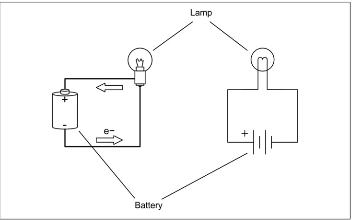
Current that flows in only one direction, as in Figure 2-4, is called direct current (DC). This is what is produced by a common battery, and by the DC power supply in a typical computer system. Current that changes direction repeatedly is called alternating

cur-rent (AC). This is what comes out of a household wall socket (in the US, for example).

It is also the type of current that drives the loudspeakers in a stereo system. The rate at which the current changes direction is called the frequency, and is measured in cycles per second in units of Hertz (abbreviated Hz). So, a 60 Hz signal is composed of a current changing direction at a rate of 60 times per second. We’ll stick to DC circuits for now, and save AC for later.

By convention, current is described as flowing from positive to ground (negative), whereas in reality electrons flow from the negative terminal to the positive terminal of the power source. In Figure 2-4, the arrows show the electron flow. Although you should be aware of this, from this point onward we’ll use the positive-to-negative con-vention for discussing current flow.

(43)

Voltage is the measure of how much electric charge, or electrical potential force, is

driving electrons into a circuit. It is measured in units of volts (V). Electric charge is a force, in that a charge will exert a force on other charged objects. How much force is exerted depends on how much charge is present. The concepts of energy, force, and potential are described by classical mechanics, and they also apply to electric charge. The main point to remember here is that a high voltage has more force than a low voltage. This is why you don’t get much more than a barely visible spark from a common flashlight battery at 1.5 volts, like the one shown in Figure 2-4, but lightning, at around 10,000,000 volts (or more!), is able to arc all the way from a cloud to the ground in a brilliant flash. The lightning has more voltage, and hence more force behind it, so it is able to overcome the insulating effects of the surrounding air.

Current is the measure of the volume of electrons moving through a circuit. What the

term current means depends on the context. As we’ve been discussing it so far, electric current refers to the flow of electric charge in a conductor, which is a physical phe-nomenon. In electronics, the word “current” is usually taken to mean the quantity of electrons flowing through a conductor at a specific point at a single instant in time. In this case, it’s referring to a physical quantity and is measured in units of amperes (A or amp).

Resistance is the measure of how much the current flow is impeded in a circuit, and it

is measured in ohms. One might think of resistance as an analog of mechanical friction (although the analogy isn’t perfect). When current flows through a resistance there is a drop in voltage across the resistance (as measured at each end), so some of the energy (voltage) in the current flow is being lost as heat. How much energy is lost is a function of how much current is flowing through the resistance and the amount of the voltage drop. As we will see very shortly, there is a famous equation that captures this rela-tionship between voltage, current, and resistance.

Power is the measure of the amount of energy consumed in overcoming the resistance

in a circuit or performing work of some sort (perhaps running a motor), and is a function of voltage and current. The common unit of measure is the watt (W), although one will occasionally see electric power expressed in terms of joules (J).

Circuit Schematics

(44)

Figure 2-6 shows the symbols for diodes (rectifiers) and transistors of various types. These are referred to as solid-state components and are considered to be active compo-nents in that they are capable of altering the current flow in a nonlinear fashion.

Figure 2-5. Common electronic schematic symbols

(45)

The wires (or circuit board traces) in a real circuit are shown as lines in a schematic. Connections between wires are shown with a solid circle where they meet; otherwise, they simply cross. This is illustrated in Figure 2-7. Some older schematic styles use a small hump in one wire to show that it doesn’t connect to the wire it is crossing, but this has become rather rare in modern diagrams. Also note that in order to avoid draw-ing multiple parallel lines to represent sets of associated wires, such as digital data buses, the bus is shown as a single heavy line with an indication of the number of individual wires involved.

(46)

Digital logic has its own set of symbols, and functions within integrated circuits (ICs) such as flip-flops, timers, registers, latches, and so on, are generally shown as rectangles with input and output connections. These types of symbols are shown in Figure 2-8.

Figure 2-8. Digital logic symbols

The set of schematic symbols presented in Figures 2-5 through 2-8 is by no means complete. A full set of all currently used schematic symbols would be much more in-volved than what is presented here. In reality, only a small subset of those symbols are necessary for our purposes.

Also, like other specialized fields, electronics is rife with its own peculiar set of abbre-viations, acronyms, and other jargon. Here is a small sampling:

DPDT

A double-pole, double-throw switch.

DPST

A double-pole, single-throw switch.

NPN

A type of transistor junction. The acronym refers to the negative-positive-negative “doping” that is used to create the active junctions where modulation of current flow occurs in the device.

PNP

The opposite of the NPN transistor. It uses positive-negative-positive junctions.

Polarity

The positive or negative state of a terminal or device.

Polarized

A device is said to be polarized when it is intended to be used such that one terminal is always more positive (or negative) than the other. Nonpolarized devices are not picky about how they are connected.

SPDT

A switch with a single pole but two active positions. May also refer to a switch with a mechanical center-off position.

SPST

A single-pole, single-throw switch.

(47)

The small “bubbles” used with digital logic symbols (as shown in Figure 2-8) indicate inversion. That is, if a logical True (1) encounters a bubble, it is inverted and becomes a logical False (0), and vice versa. For example, the truth table for an AND device (where A and B are the inputs) is shown in Table 2-1.

Table 2-1. AND gate logic

A B Output

0 0 0

0 1 0

1 0 0

1 1 1

The NAND (Not-AND) device, with a bubble on the output, produces the truth table shown in Table 2-2.

Table 2-2. NAND gate logic

A B Output

0 0 1

0 1 1

1 0 1

1 1 0

Don’t be confused by the open circles often used to indicate terminal points in a circuit diagram. These do not indicate logical inversion. Only when the open circle is next to a digital component symbol does it mean that logical inversion is applicable.

Schematic symbols will be introduced or revisited as we go along, so there’s no need to commit these to memory at this point. If you’re curious, I encourage you to inves-tigate the references found at the end of this chapter for more details on schematics and the various symbols utilized in creating them.

DC Circuit Characteristics

Now let’s examine the lamp and battery circuit in Figure 2-4 more closely. It may seem simple, but there is actually quite a bit going on here.

(48)

When electrical current flows through a circuit, there is always some amount of resist-ance to the flow; even wires have some resistresist-ance. A circuit with low resistresist-ance will move current more easily than a circuit with high resistance, and the high-resistance circuit will require a higher voltage to achieve the same level of current flow as the low-resistance circuit. For example, a circuit with a 10-volt supply and 50 ohms of low-resistance will conduct 0.2 A (also stated as 200 mA, or milliamps—thousandths of an ampere) of current. If the resistance is increased to 100 ohms and we still want to maintain 200 mA of current, the voltage will need to be increased to 20 volts. A high-resistance circuit will also dissipate more power (heat) than a low-resistance circuit at the same current. We’ll have more to say about this a little later.

Ohm’s Law

As you may have already surmised, there is a fundamental relationship between voltage, current, and resistance. This is called Ohm’s law, and it looks like this:

E = IR

where E is voltage, I is current, and R is resistance. This simple equation is fundamental to electronics, and indeed it is the only equation that one really needs to accomplish many instrumentation implementations.

In Figure 2-4, the circuit has only two components: a battery and a lamp. The lamp composes what is called the “load” in the circuit. Incandescent lamps have a resistance that varies according to temperature, but for our purposes we’ll assume that the lamp has a resistance of 2 ohms when it is glowing brightly. The battery is 1.5 volts, and we’ll assume that it is capable of delivering a maximum current of 500 milliamps for one hour (this is the battery’s total capacity, which is usually around 0.5 amp/hr for a typical AA type battery) at its rated output voltage.

According to Ohm’s law, the amount of current the lamp will draw from the battery is given by:

I = E/R

or:

I = 1.5/2

I = 0.75A

Here, the value for I can also be written as 750 mA (milliamperes). If we want to know how long the battery will last, we can divide its capacity by the current in the circuit:

0.5/0.75 = 0.67 hours (approximately)

(49)

This might explain why those cute little single-AA-battery flashlights sometimes handed out at trade shows don’t last very long before a new battery is needed. In the simple circuit shown in Figure 2-4, the flow of electrons through the filament in the lamp causes it to heat up to the point where it glows brightly (1600 to 2800°C or so). The filament in the lamp gets hot because it has resistance, so current flows less easily through the filament than it does through the wires in the circuit. The power expended to force the current through the filament is expressed as heat. The energy converted and dissipated by a component is defined in terms of dissipated power and is expressed in watts (W). Power in a DC circuit is computed by multiplying the voltage by the current, like so:

P = EI

If we want to know how much power the lightbulb in our circuit is consuming, we simply multiply the voltage across the bulb by the current:

P = 1.5 * 0.75P = 1.125 watts

Now let’s look at a slightly more complicated circuit with some new symbols. Consider the simple LED circuit shown in Figure 2-9. Here we have a resistor in series with an LED (light-emitting diode). There is a 5-volt DC power supply indicated but not shown, and a ground connection (which is the current flow return back to the power supply).

Figure 2-9. Simple LED circuit

(50)

Since we can assume a 1.7 V drop for the LED, we can also assume a 3.3 V drop across the resistor. If we solve Ohm’s law for R, we get:

R = E/I

R = 3.3/0.01

R = 330 ohms

So, a resistor with a value of 330 ohms will supply the 10 mA of current the LED needs to conduct and start glowing. This simple example is more important than you might think, and it will pop up again when we look into connecting LEDs to discrete digital I/O ports later.

Sinking and Sourcing

When reviewing the specifications for an interface device, one may encounter ratings for current sink and source capabilities. What this means, essentially, is that when a load is connected from the device to the positive power source, the device will be able to “sink” up to the specified amount of current before risking damage. Conversely, when the load is connected from the device to ground, it will be able to safely “source” up to the rated amount of current. Figure 2-10 shows this schematically.

The step up and step down symbols indicate how the LED will respond when the voltage from the device is high or low. When the output of the device is low with respect to the +5 V supply the LED in the current sink configuration will be active, and when it is high with respect to ground the LED will be active in the current source arrange-ment. The same math we used to determine the value of R for Figure 2-9 applies here as well. Note that it is important not to exceed a device’s maximum sink or source ratings. For example, when a device is rated for 20 mA of current source capability, it may mean 20 mA for the whole device, not just for a single output pin.

More About Resistors

Resistors are ubiquitous in electronic circuits. A resistor can be fabricated from a piece of a poorly conductive carbon material, from a carbon film deposited on a ceramic core, or from a section of resistive wire wound inside a protective package of some type. In addition to a specific resistance value (in ohms), resistors also have a wattage rating. Typical values are 1/10, 1/8, 1/4, 1/2, 1, 2, and 5 watts, with even larger ratings available for special-purpose applications. This sets the maximum amount of power the device can safely dissipate before it risks self-destruction. Lastly, resistors are manufactured to specific tolerances, ranging from 20% to less than 1%, with the price rising as the tolerance tightens. The most common tolerance value is 5%.

(51)

Figure 2-10. Current sink and current source

Figure 2-11 shows a generic resistor. Notice that this type of resistor uses color bands to denote its value. You can find the resistor color code in any basic electronics text, and it is explained on numerous websites, so we won’t go into it here.

(52)

Resistors can be used to reduce a voltage level or limit the current in a circuit, among other things. Resistors are often found in instrumentation applications in circuits such as the one in Figure 2-9, in the role of current limiter. Resistors can be used singly, or they can be connected in parallel or serial configurations. Figure 2-12 shows both, and the simple math used to calculate the equivalent resistances.

Figure 2-12. Series and parallel resistance

We now have enough pieces of the DC puzzle to start to do useful and interesting things with voltage, current,