The Multistrand Simulator: Stochastic Simulation of the Kinetics of Multiple Interacting DNA Strands

(1)

Kinetics of Multiple Interacting DNA Strands

Thesis by

Joseph Malcolm Schaeffer

In Partial Fulfillment of the Requirements

for the Degree of

Master of Science

California Institute of Technology

Pasadena, California

2012

(2)

c

2012

Joseph Malcolm Schaeffer

(3)

Acknowledgements

Thanks to my advisor Erik Winfree, for his enthusiasm, expertise and encouragement. The

models presented here are due in a large part to helpful discussions with Niles Pierce,

Robert Dirks, Justin Bois and Victor Beck. Two undergraduates, Chris Berlind and Jashua

Loving, did summer research projects based on Multistrand and in the process helped

build and shape the simulator. There are many people who have used Multistrand and

provided very helpful feedback for improving the simulator, especially Josh Bishop, Nadine

Dabby, Jonathan Othmer, and Niranjan Srinivas. Thanks also to the many past and current

members of the DNA and Natural Algorithms group for providing a stimulating environment

in which to work.

There are many medical professionals to which I owe my good health while writing this

thesis, especially Dr. Jeanette Butler, Dr. Mariel Tourani, Cathy Evaristo, and the staff of

the Caltech Health Center, especially Alice, Divina and Jeannie.

I want to acknowledge all my family and friends for their support. A journey is made

all the richer for having good company, and I would not have made it nearly as far without

all the encouragement.

Finally, I must thank my wife Lorian, who has been with me every step of this journey

(4)

Abstract

DNA nanotechnology is an emerging field which utilizes the unique structural properties of

nucleic acids in order to build nanoscale devices, such as logic gates, motors, walkers, and

algorithmic structures. These devices are built out of DNA strands whose sequences have

been carefully designed in order to control their secondary structure - the hydrogen bonding

state of the bases within the strand (called “base-pairing”). This base-pairing is used to

not only control the physical structure of the device, but also to enable specific interactions

between different components of the system, such as allowing a DNA walker to take steps

along a prefabricated track. Predicting the structure and interactions of a DNA device

requires good modeling of both the thermodynamics and the kinetics of the DNA strands

within the system. Thermodynamic models can be used to make equilibrium predictions

for these systems, allowing us to look at questions like “Is the walker-track interaction a

well-formed and stable molecular structure?”, while kinetics models allow us to predict the

non-equilibrium dynamics, such as “How quickly will the walker take a step?”. While the

thermodynamics of multiple interacting DNA strands is a well-studied model which allows

for both analysis and design of DNA devices, previous work on the kinetics models only

explored the kinetics of how a single strand folds on itself.

The kinetics of a set of DNA strands can be modeled as a continuous time Markov

process through the state space of all secondary structures. Due to the exponential size

of this state space it is computationally intractable to obtain an analytic solution for most

problem sizes of interest. Thus the primary means of exploring the kinetics of a DNA

system is by simulating trajectories through the state space and aggregating data over

many such trajectories. We developed the the Multistrand kinetics simulator, which extends the previous work by including the multiple strand version of the thermodynamics

model (a core component for calculating parameters of the kinetics model), extending the

(5)

by adding new kinetic moves that allow interactions between distinct strands. Furthermore,

we prove that our modified thermodynamic and kinetic models are exactly equivalent to

the canonical thermodynamics model when the simulation is run for sufficiently long time

to reach equilibrium.

The kinetic simulator was implemented in C++ for time critical components and in

Python for input and output routines as well as post-processing of trajectory data. A key

contribution of this work was the development of data structures and algorithms that take

advantage of local properties of secondary structures. These algorithms enable the efficient

reuse of the basic objects that form the system, such that only a very small part of the state’s

neighborhood information needs to be recalculated with every step. Another key addition

was the implementation of algorithms to handle the new kinetic steps that occur between

different DNA strands, without increasing the time complexity of the overall simulation.

These improvements led to a reduction in worst case time complexity of a single step being

just quadratic in the input size (the number of bases in the simulated system), rather than

cubic, and also led to additional improvements in the average case time complexity.

What data does the simulation produce? At the very simplest, the simulation produces

a full kinetic trajectory through the state space - the exact states it passed through, and

the time at which it reached them. A small system might produce trajectories that pass

through hundreds of thousands of states, and that number increases rapidly as the system

gets larger! Going back to our original question, the type of information a researcher hopes

to get out of the data could be very simple: “How quickly does the walker take a step?”, with

the implied question of whether it’s worth it to actually order the particular DNA strands

composing the walker, or go back to the drawing board and redesign the device. One way

to acquire that type of information is to look at the first time in the trajectory where we

reached the “walker took a step” state, and record that information for a large number of

simulated trajectories in order to obtain a useful answer. We designed and implemented

new simulation modes that allow the full trajectory data to be condensed as it’s generated

into only the pieces the user cares about for their particular question. This analysis tool

also required the development of flexible ways to talk about states that occur in trajectory

data; if someone wants data on when the walker took a step, we have to be able to express

(6)

List of Figures

3.1 Secondary structure divided into loops. . . 8

4.1 Adjacent Microstate Diagram . . . 12

5.1 Representation of Secondary Structures . . . 21

5.2 Move Data Structure . . . 23

5.3 Move Update (example) . . . 26

5.4 Move Generation (example) . . . 28

5.5 Full comparison vs Kinfold 1.0 . . . 30

6.1 Trajectory Data . . . 33

6.2 Three way branch migration system . . . 34

6.3 Trajectory Output after 0.01 s simulated time. . . 35

6.4 Trajectory Output after 0.05 s simulated time. . . 36

6.5 Example Macrostate . . . 39

6.6 Hairpin Folding Pathways . . . 42

6.7 First Passage Time Data, Design B . . . 47

6.8 First Passage Time Data, Design A . . . 49

6.9 First Passage Time Data, Sequence Design Comparison . . . 49

6.10 First Passage Time Data, 6 Base Toeholds . . . 50

6.11 Starting Complexes and Strand labels . . . 52

6.12 Final Complexes and Strand labels . . . 52

A.1 Relationships between data structure components . . . 58

D.1 Polymer Graph Representation . . . 107

(10)

(11)

Chapter 1

Introduction

DNA nanotechnology is an emerging field which utilizes the unique structural properties

of nucleic acids in order to build nanoscale devices, such as logic gates [18], motors [4, 1],

walkers [19, 1, 20], and algorithmic structures [14, 23]. These devices are built out of DNA

strands whose sequences have been carefully designed in order to control their secondary

structure - the hydrogen bonding state of the bases within the strand (called “base-pairing”).

This base-pairing is used to not only control the physical structure of the device, but also

to enable specific interactions between different components of the system, such as allowing

a DNA walker to take steps along a prefabricated track. Predicting the structure and

interactions of a DNA device requires good modeling of both the thermodynamics and the

kinetics of the DNA strands within the system. Thermodynamic models can be used to

make equilibrium predictions for these systems, allowing us to look at questions like “Is

the walker-track interaction a well-formed and stable molecular structure?”, while kinetics

models allow us to predict the non-equilibrium dynamics, such as “How quickly will the

walker take a step?”. While the thermodynamics of multiple interacting DNA strands is

a well-studied model [5] which allows for both analysis and design of DNA devices [24, 6],

previous work on secondary structure kinetics models only explored the kinetics of how a

single strand folds on itself [7].

The kinetics of a set of DNA strands can be modeled as a continuous time Markov

pro-cess through the state space of all secondary structures. Due to the exponential size of this

state space it is computationally intractable to obtain an analytic solution for most problem

sizes of interest. Thus the primary means of exploring the kinetics of a DNA system is by

simulating trajectories through the state space and aggregating data over many such

(12)

work [7] by using the multiple strand thermodynamics model [5] (a core component for

cal-culating transition rates in the kinetics model), adding new terms to the thermodynamics

model to account for stochastic modeling considerations, and by adding new kinetic moves

that allow bimolecular interactions between strands. Furthermore, we prove that this new

kinetics and thermodynamics model is consistent with the prior work on multiple strand

thermodynamics models [5].

The Multistrand simulator is based on the Gillespie algorithm [8] for generating sta-tistically correct trajectories of a stochastic Markov process. We developed data structures

and algorithms that take advantage of local properties of secondary structures. These

algo-rithms enable the efficient reuse of the basic objects that form the system, such that only a

very small part of the state’s neighborhood information needs to be recalculated with every

step. A key addition was the implementation of algorithms to handle the new kinetic steps

that occur between different DNA strands, without increasing the time complexity of the

overall simulation. These improvements lead to a reduction in worst case time complexity

of a single step and also led to additional improvements in the average case time complexity.

What data does the simulation produce? At the very simplest, the simulation produces

a full kinetic trajectory through the state space - the exact states it passed through, and

the time at which it reached them. A small system might produce trajectories that pass

through hundreds of thousands of states, and that number increases rapidly as the system

gets larger. Going back to our original question, the type of information a researcher hopes

to get out of the data could be very simple: “How quickly does the walker take a step?”,

with the implied question of whether it’s worth it to actually purchase the particular DNA

strands composing the walker to perform an experiment, or go back to the drawing board

and redesign the device. One way to acquire that type of information is to look at the first

time in the trajectory where we reached the “walker took a step” state, and record that

information for a large number of simulated trajectories in order to obtain a useful answer.

We designed and implemented new simulation modes that allow the full trajectory data to

be condensed as it’s generated into only the pieces the user cares about for their particular

question. This analysis tool also required the development of flexible ways to talk about

states that occur in trajectory data; if someone wants data on when the walker took a step,

we have to be able to express that in terms of the Markov process states which meet that

(13)

Chapter 2

System

We are interested in simulating nucleic acid molecules (DNA or RNA) in a stochastic regime;

that is to say that we have a discrete number of molecules in a fixed volume. This regime is

found in experimental systems that have a small volume with a fixed count of each molecule

present, such as the interior of a cell. We can also apply this to experimental systems with

a larger volume (such as a test tube) when the system is well mixed, as we can pick a fixed

(small) volume and deal with the expected counts of each molecule within it, rather than

the whole test tube.

To discuss the modeling and simulation of the system, we need to be very careful to

define the components of the system, and what comprises a state of the system within the

simulation.

2.1

Strands

Each DNA molecule to be simulated is represented by a strand. Our system then contains a set of strands Ψ∗, where each strand s ∈ Ψ∗ is defined by s = (id, label, sequence). A

strand’siduniquely identifies the strand within the system, while thesequenceis the ordered list of nucleotides that compose the strand.

Two strands could be considered identicalif they have the same sequence. However, in some cases it is convenient to make a distinction between strands with identical sequences.

For example, if one strand were to be labelled with a fluorophore, it would no longer be

physically identical to another with the same sequence but no fluorophore. Thus, thelabel

is used to designate whether two strands are identical. We define two strands as being

(14)

the label and the sequence is not used, so it will be explicitly noted when it is important.

2.2

Complex Microstate

Acomplexis a set of strands connected by base pairing (secondary structure). We define the state of a complex byc= (ST, π∗, BP), called the “complex microstate”. The components

are a nonempty set of strands ST ⊆Ψ∗, an ordering π∗ on the strands ST, and a list of

base pairingsBP ={(ij·kl)| baseion strandj is paired to basek on strandl, and j≤l,

withi < kifj=l}, where we note that “strandl” refers to the strand occuring in position

lin the orderingπ∗. Note that we require a complex to be “connected”: there is no proper

subset of strands in the complex for which the base pairings involving those strands do not

involve at least one base outside that subset. Given a complex microstate c, we will use

ST(c), π∗(c), BP(c) to refer to the individual components.

While this definition defines the full space of complex microstates, it is common to

disal-low some secondary structures due to physical or computational constraints. For example,

we disallow the pairing of a base with any other within three bases on the same strand, as

this would correspond to an impossible physical configuration. Another class of disallowed

structures are called thepseudoknottedsecondary structures, which require computationally difficult energy model calculations, and are fully defined and discussed further in Section

D.

2.3

System Microstate

A system microstate represents the configuration of the strands in the volume we are

sim-ulating (the “box”). Since we allow complexes to be formed of one or more strands, every

unique strand in the system must be present in a single complex and thus we can represent

the system microstate by a set of those complexes.

We define a system microstate ias a set of complex microstates, such that each strand in the system is in exactly one complex within the system. This is formally stated in the

(15)

[

c∈i

ST(c) = Ψ∗ and ∀c, c0 ∈iwithc=6 c0, ST(c)∩ST(c0) =∅ (2.1)

This definition leads to the natural use of|i|to indicate the number of complexes present

in system microstate i, and i\j to indicate the complex microstates present in system

(16)

Chapter 3

Energy

The conformation of a nucleic acid strand at equilibrium can be predicted by a well studied

model, called the nearest neighbor energy model [16, 15, 17]. Recent work has extended

this model to cover systems with multiple interacting nucleic acid strands [5].

The distribution of system microstates at equilibrium is a Boltzmann distribution, where

the probability of observing a microstate iis given by

P r(i) = 1 Q ∗e

−∆Gbox(i)/RT _(3.1)

where ∆Gbox(i) is the free energy of the system microstate i, and is the key quantity

determined by these energy models. Q=P

ie

−∆Gbox(i)/RT _{is the partition function of the}

system, R is the gas constant, andT is the temperature of the system.

3.1

Energy of a System Microstate

We now consider the energy of the system microstatei, and break it down into components.

The system consists of many complex microstates c, each with their own energy. We also

must account for the entropy of the system (the number of configurations of the complexes

spatially within the “box”) in the energy, and thus must define these two terms.

Let us first consider the entropy term. We consider the “zero” energy system microstate

to be the one in which all strands are in separate complexes, thus our entropy term is in

(17)

that the number of complexes in the system,N, is much smaller than the number of solvent

molecules within our box, Ms. We can then approximate the standard statistical entropy

of the system as N∗RT logMs. Letting K be the total number of strands in the system,

our zero state is then K ∗RT logMs. Defining ∆Gvolume =RT logMs, the contribution

to the energy of the system microstate ifrom the entropy of the box is then:

(K−N)∗∆Gvolume

And thus in terms of N, K,∆Gvolume and ∆G(c) (the energy of complex microstate c,

defined in the next section), we define ∆Gbox(i), the energy of the system microstate i, as

follows:

∆Gbox(i) = (K−N)∗∆Gvolume+

X

c∈i

∆G(c)

Before we turn our attention to the energy of a complex microstate, let us examine a

situation where we are modeling a fixed volume of a larger solution, and how that relates to

the quantity Ms. If we assume that the volume studied isV (units of liters), we can easily

compute the number of solvent molecules in this volume using the densityd of water (the

solvent, ing/L) , the molar mass M of water (in grams per mol), and Avogadro’s number,

as follows: Ms = V_M∗d ∗NA. In practice, we may wish to choose a simulation volume V

based on other physical quantities, such as the concentration of a single molecule within

the volume1.

The energy formulas derived here, suitable for our stochastic model, differ from those in

[5] in two main ways: the lack of symmetry terms, and the addition of the ∆Gvolume term.

We compare this stochastic model to the mass action model in much more detail in Section

C.

1

CalculatingMs from a concentrationuin mol/L of a single molecule in the volume is straightforward.

We assume that our concentrationuimplies the volumeV is chosen corresponding to exactly one molecule being present in that volume, as follows:V = _u_∗1_N

A and thusMs=

d M∗u=

ρ_H

2O

(18)

3.2

Energy of a Complex Microstate

We previously defined a complex microstate in terms of the list of base pairings present

within it. However, the well studied models are based upon nearest neighbor interactions

between the nucleic acid bases. These interactions divide the secondary structure of the

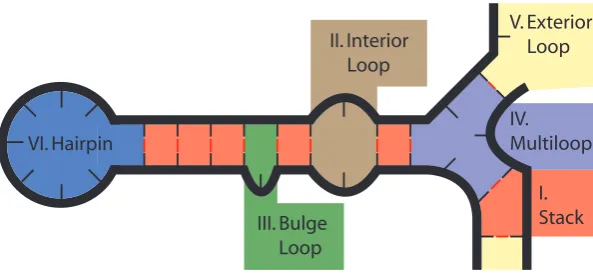
system into local components which we refer to asloops, shown in figure 3.1.

IV. Multiloop V. Exterior Loop I. Stack III. Bulge Loop II. Interior Loop VI. Hairpin

Figure 3.1: Secondary structure divided into loops.

These loops can be broken down into different categories, and parameter tables for each

category have been determined from experimental data [17]. Each loop l has an energy,

∆G(l) which can be retrieved from the appropriate parameter table for its category, which

is discussed in more detail in section B.3. Each complex also has an energy contribution

associated with the entropic initiation cost [3] (e.g. rotational) of bringing two strands

together, ∆Gassoc, and the total contribution is proportional to the number of strands L

within the complex, as follows 2: (L−1)∗∆Gassoc.

2

The free energy ∆G◦ for a reaction A+B −)*− C is usually expressed in terms of the equilib-rium constant Keq and the concentrations [A],[B],[C] (in mol/L) of the molecules involved, as follows:

e∆G◦/RT = Keq = [A_[_C][B_]]. We can also express the free energy ∆G0 in terms of the dimensionless

mole fractions xA, xB, xC, where xi = [i]/ρH2O (for dilute solutions), and ρH2O is the molarity of wa-ter. In this case, we havee∆G0/RT =Keq0 = xA

∗xB

xC , and relating it to the previous equation, we see that

e∆G0/RT ₌ ([A]/ρH2O)∗([B]/ρH2O)

[C]∗ρH2O =

[A][B] [C] ∗

1

ρH2O =e

∆G◦/RT_∗_e−logρH2O_{. Thus if we have an energy ∆}_G◦

which was for concentration units and we wish to use mole fraction units, we must adjust it by−RTlogρH2O to obtain the correct quantity. In general, if we have a complex ofN molecules, the conversion to mole frac-tions will require an adjustment of −(N−1)∗RTlogρH2O. To be consistent with [5], we wish to always use free energies which are based on the mole fraction units, and thus must include this factor since the reference free energies are for concentration units. In [5], the factor is included in the ∆Gassoc term, and

thus we include it in the same place, as follows: ∆Gassoc= ∆Gpubassoc−RTlogρH2O, where ∆Gpubassocis found

(19)

The energy of a complex microstatecis then the sum of these two types of contributions.

We can also divide any free energy ∆G into the enthalpic and entropic components, ∆H

and ∆S related by ∆G = ∆H + T ∗∆S, where T is the temperature of the system.

For a complex microstate, each loop can have both enthalpic and entropic components,

but ∆Gassoc is usually assumed to be purely entropic [16]. This becomes important when

determining the kinetic rates, in section 4.

We use ∆G(c) to refer to the energy of a complex microstate to be consistent with the

nomenclature in [5], where ∆G(c) refers to the energy of a complex when all strands within

it are consider unique (as is the case in our system), and ∆G(c) is the energy of the

com-plex, without assuming that all strands are unique (and thus it must account for rotational

symmetries). This is discussed more in Section C.

In summary, the standard free energy of a complex microstatec, containingL=|ST(c)|

strands:

∆G(c) =



 X

loop l∈c

∆G(l)



+ (L−1)∆Gassoc

3.3

Computational Considerations

While the simulator could use the system microstate energy in the form given in the previous

sections, it is convenient for us to group terms such that the computation need only take

place per complex. Thus we wish to include the (K −N)∆Gvolume term in the energy

computation for the complex microstates. Recall that K is the number of strands in the

system, andN is the number of complexes in the system microstate. Assuming that we are

(20)

K = X

c∈i

|ST(c)|

N = X

c∈i

1

And thus arrive at:

∆Gbox(i) =

X

c∈i

∆G(c) + (|ST(c)| −1)∗∆Gvolume

We then define ∆G∗(c) = ∆G(c) + (|ST(c)| −1)∗∆Gvolume, andLc=|ST(c)|and thus

have the following forms for the energy of a system microstate and the energy of a complex

microstate:

∆Gbox(i) =

X

c∈i

∆G∗(c)

∆G∗(c) =



 X

loop l∈c

∆G(l)



+ (Lc−1)∗(∆Gassoc+ ∆Gvolume)

Since we expect the probability of observing a particular complex microstate to remain

the same no matter what reference units we use for the free energy (see footnote 2), this

implies that if we wanted to express our ∆G∗(c) for concentration units, we would use

∆Gassoc = ∆Gpubassoc and ∆Gvolume =RTlogρMH2sO = RTlog

1

u = RTlog V

V0, where u is the molar concentration of a single molecule in the box volume V, andV0 is the volume for 1

(21)

Chapter 4

Kinetics

4.1

Basics

Thermodynamic predictions have only limited use for some systems of interest, if the key

information to be gathered is the reaction rates and not the equilibrium states. Many

systems have well defined ending states that can be found by thermodynamic prediction,

but predicting whether it will reach the end state in a reasonable amount of time requires

modeling the kinetics. Kinetic analysis can also help uncover poor sequence designs, such

as those with alternate reactions leading to the same states, or kinetic traps which prevent

an intended reaction from occurring quickly.

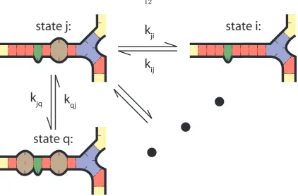
The kinetics are modeled as a continuous time Markov process over secondary structure

space. System microstates i, j are considered adjacent if they differ by a single base pair

(Figure 4.1), and we choose the transition rates kij (the transition from state ito state j)

and kji such that they obey detailed balance:

kij

kji

=e−

∆_Gbox(j)−∆_Gbox(i)

RT (4.1)

This property ensures that given sufficient time we will arrive at the same equilibrium

state distribution as the thermodynamic prediction, (i.e. the Boltzmann distribution on

system microstates, equation 3.1) but it does not fully define the kinetics as this only

constrains the ratio kij

kji. We discuss how to choose these transition rates in the following

sections, but regardless of this choice, we can still determine how the next state is chosen

(22)

state j:

state i:

state q:

k

_ji

k

_ij

k

_qj

k

_jq

Figure 4.1: System microstatesi, qadjacent to current statej, with many others not shown.

Given that we are currently in state i, the next state m in a simulated trajectory is

chosen randomly among the adjacent states j, weighted by the rate of transition to each.

P r(m) = kim Σjkij

(4.2)

Similarly, the time taken to transition to the next state is chosen randomly from an

exponential distribution with rate parameter λ, whereλis the total rate out of the current

state, Σjkij.

P r(∆t) =λexp(−λ∆t) (4.3)

We will now classify transitions into two exclusive types: those that change the number

of complexes present in the system, calledbimolecular transitions, and those where changes

(23)

4.2

Unimolecular Transitions

Because unimolecular transitions involve only a single complex, it is natural to define these

transitions in terms of the complex microstate which changed, rather than the full system

microstate. Like Figure 4.1 implies, we define a complex microstate das being adjacent to

a complex microstate c if it differs by exactly one base pair. We call a transition from c

to d that adds a base pair a creation move, and a transition from c to d that removes a

base pair adeletionmove. The exclusion of pseudoknotted structures is not inherent in this definition of adjacent states, but rather arises from our disallowing pseudoknotted complex

microstates.

In more formal terms we now define the adjacent states to a system microstate, rather

than those adjacent to a complex microstate as in the simple definition above. Recall from

section 2.3 that |i|is the number of complexes present in system microstate i, and i\j is

the set of complex microstates inithat are not also in system microstatej.

Two system microstates i, j are adjacent by a unimolecular transition iff ∃c ∈i, d ∈j

such that:

|i|=|j|and i\j={c}and j\i={d} (4.4)

and one of these two holds:

BP(c)⊂BP(d) and |BP(d)|=|BP(c)|+ 1 (4.5)

BP(d)⊂BP(c) and |BP(c)|=|BP(d)|+ 1 (4.6)

In other words, the only differences between i and j are in c and d, and they differ by

exactly one base pair. If equation 4.5 is true, we call the transition fromi toj a base pair creation move, and if equation 4.6 is true, we call the transition from i to j a base pair

deletion move. Note that if itoj is a creation move, j toi must be a deletion move, and vice versa. Similarly, if there is no transition fromitoj, there cannot be a transition from

(24)

4.3

Bimolecular Transitions

A bimolecular transition from system microstateito system microstate j is one where the

single base pair difference between them leads to a differing number of complexes within

each system microstate. This differing number of complexes could be due to a base pair

joining two complexes in i to form a single complex in j, which we will call a join move. Conversely, the removal of this base pair from icould cause one complex inito break into

two complexes withinj, which we will call abreak move. Note that ifitoj is a join move, thenj toimust be a break move, and vice versa. As we saw before, this also implies that

every bimolecular move is reversible.

Formally, a transition from system microstateito system microstate j is a join move if

|i|=|j|+ 1 and we can find complex microstatesc, c0 ∈iand d∈j, with c6=c0 such that

the following equations hold:

i\ {c, c0}=j\ {d} (4.7)

∃x∈BP(d) s.t. BP(d)\ {x}=BP(c)∪BP(c0) (4.8)

Similarly, a transition from system microstate ito system microstatej is a break move

if|i|+ 1 =|j|and we can find complex microstatesc∈iandd, d0∈j withd6=d0 such that

the following equations hold:

i\ {c}=j\ {d, d0} (4.9)

∃x∈BP(c) s.t. BP(c)\ {x}=BP(d)∪BP(d0) (4.10)

While arbitrary bimolecular transitions are not inherently prevented from forming

pseu-doknots in this model, we again implicitly prevent them by using only complex microstates

(25)

4.4

Transition Rates

Now that we have defined all of the possible transitions between system microstates, we

must decide how to assign rates to each transition. We know that if there is a transition

from system microstate i to system microstate j with rate kij there must be a transition

from j toiwith rate kji which are related by:

kij

kji

=e−

RT (4.11)

This condition is known as detailed balance, and does not completely define the rates kij, kji. Thus a key part of our model is the choice of rate method, the way we set the rates

of a pair of reactions so that they obey detailed balance.

While our simulator can use any arbitrary rate method we can describe, we would like

our choice to be physically realistic (i.e. accurate and predictive for experimental systems).

There are several rate methods found in the literature [10, 11, 26] which have been used for

kinetics models for single-stranded nucleic acids [7, 26] with various energy models. As a

start, we have implemented three of these simple rate methods which were previously used

in single base pair elementary step kinetics models for single stranded systems. In addition

we present a rate method for use in bimolecular transitions that is physically consistent

with both mass action and stochastic chemical kinetics. We verify that the kinetics model

(and thus our choice of rate method) have been correctly implemented by verifying that the

detailed balance condition holds (Section 6.1.2).

In order to maintain consistency with known thermodynamic models, each pair ofkij and

kji must satisfy detailed balance and thus their ratio is determined by the thermodynamic

model, but in principle each pair could be independently scaled by some arbitrary prefactor,

perhaps chosen to optimize agreement with experimental results on nucleic acid kinetics.

However, since the number of microstates is exponential, this leads to far more model

parameters (the prefactors) than is warranted by available experimental data. For the time

being, we limit ourselves to using only two scaling factors: kuni for use with unimolecular

(26)

4.5

Unimolecular Rate Models

The first rate model we will examine is the Kawasaki method [10]. This model has the

property that both “downhill” (energetically favorable) and uphill transitions scale directly

with the steepness of their slopes.

kij = kuni∗e−

2RT (4.12)

kji = kuni∗e−

∆_Gbox(i)−∆_Gbox(j)

2RT (4.13)

The second rate model under consideration is the Metropolis method [11]. In this model,

all downhill moves occur at the same fixed rate, and only the uphill moves scale with the

slope. This means that the maximum rate for any move is bounded, and in fact all downhill

moves occur at this rate. This is in direct contrast to the Kawasaki method, where there is

no bound on the maximum rate.

if ∆Gbox(i)>∆Gbox(j) then kij = 1∗kuni (4.14)

kji= kuni∗e−

∆_Gbox(i)−∆_Gbox(j)

RT (4.15)

otherwise, kij = kuni∗e−

RT (4.16)

kji= 1∗kuni (4.17)

Finally, the entropy/enthalpy method [26] uses the division of free energies into entropic

and enthalpic components to assign the transition rates in an intuitive manner: base pair

creation moves must overcome the entropic energy barrier to bring the bases into contact,

and base pair deletion moves must overcome the enthalpic energy barrier in order to break

(27)

ifitoj is a creation: kij = kuni∗e

∆_Sbox(j)−∆_Sbox(i)

R (4.18)

kji= kuni∗e−

∆_Hbox(i)−∆_Hbox(j)

RT (4.19)

otherwise, kij = kuni∗e−

∆_Hbox(j)−∆_Hbox(i)

RT (4.20)

kji= kuni∗e

∆_Sbox(i)−∆_Sbox(j)

R (4.21)

We note that the value of kuni that best fits experimental data is likely to be different

for all three models.

4.6

Bimolecular Rate Model

When dealing with moves that join or break complexes, we must consider the choice of how

to assign rates for each transition in a new light. In the particular situation of the join

move, where two molecules in a stochastic regime collide and form a base pair, this rate is

expected to be modeled by stochastic chemical kinetics.

Stochastic chemical kinetics theory [8] tells us that there should be a rate constant k

such that the propensity of a particular bimolecular reaction between two species Xand Y

should bek∗#X∗#Y /V, where #X and #Y are the number of copies ofX andY in the

volume V. Since our simulation considers each strand to be unique, #X = #Y = 1, and

thus we see the propensity should scale as 1/V. Recalling that ∆Gvolume =RTlog(V ∗y),

where y is a collection of constant terms (discussed in Section 3.1) andV is the simulated

volume, we see that we can obtain the 1/V scaling by letting the join rate be proportional

toe−∆Gvolume/RT_.

Thus, we arrive at the following rate method, and note that the choice of k (above) or

our scalar termkbican be found by comparison to experiments measuring the hybridization

(28)

ifitoj is a complex join move: kij = kbi∗e

−∆_Gvolume

RT (4.22)

kji = kbi∗e−

∆_Gbox(i)−∆_Gbox(j)+∆_Gvolume

RT (4.23)

otherwise, kij = kbi∗e−

∆_Gbox(j)−∆_Gbox(i)+∆_Gvolume

RT (4.24)

kji = kbi∗e−

∆_Gvolume

RT (4.25)

This formulation is convenient for simulation, as the join rates are then independent

of the resulting secondary structure. We could use the other choices for assigning rates

from 4.4, but they would require much more computation time. While the above model

is of course an approximation to the physical reality (albeit one which we believe at least

intuitively agrees with what we expect from stochastic chemical kinetics), if we later

deter-mine there is a better approximation we could use that instead, even if it cost us a bit in

computation time. One issue in the above model that we wish to revisit in the future is that

due to the rate being determined foreverypossible first base pair between two complexes, the overall rate for two complexes to bind (by a single base pair) is proportional roughly

(29)

Chapter 5

The Simulator : Multistrand

Energy and kinetics models similar to these can been solved analytically; however, the

standard master equation methods [22] scale with the size of the system’s state space. For

our DNA secondary structure state space, the size gets exponentially large as the strand

length increases, so these methods become computationally prohibitive. One alternate

method we can use is stochastic simulation [8], which has previously been done for

single-stranded DNA and RNA folding (the Kinfold simulator [7]). Our stochastic simulation refines these methods for our particular energetics and kinetics models, which extends the

simulator to handle systems with multiple strands and takes advantage of the localized

energy model for DNA and RNA.

5.1

Data Structures

There are two main pieces that go into this new stochastic simulator. The first piece is

the multiple data structures needed for the simulation: theloop graphwhich represents the complex microstates contained within a system microstate (Section 5.1.2), themoves which

represent transitions in our kinetics model – the single base pair changes in our structure

that are the basic step in the Markov process, and the move tree the container for moves

that lets us efficiently store and organize them (Section 5.1.3).

5.1.1 Energy Model

Since the basic step for calculating the rate of a move involves the computation of a state’s

energy, we must be able to handle the energy model parameter set in a manner that simplifies

(30)

described, though without the extension to multiple strand systems. While the format of

the parameter set that is used remains the same, we must implement an interface to this

data which allows us to quickly compute the energy for particular loop structures (local

components of the secondary structure, described in 3.2). This allows us to do the energy

computations needed to compute the kinetic rates for individual components of the system

microstate, allowing us to use more efficient algorithms for recomputing the energy and

moves available to a state after each Markov step.

The energy model parameter set and calculations are implemented in a simple modular

data structure that allows for both the energy computations at a local scale as we have

previously mentioned, but also as a flexible subunit that can be extended to handle

en-ergy model parameter sets from different sources. In particular, we have implemented two

particular parameter set sources: the NUPACK parameter set [24] and the Vienna RNA

parameters [9] (which does not include multistranded parameters, so defaults for those are

used). Adding new parameter set sources (such as the mfold parameters [27]) is a simple

extension of the existing source code. Additionally, the energy model interface allows for

easy extension of existing models to handle new situations, e.g. adding a sequence

depen-dent term for long hairpins. We hope this energy model interface will be useful for future

research where authors may wish to simulate systems with a unique energy model and

kinetics model.

5.1.2 The Current State: Loop Structure

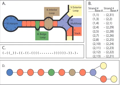
A system microstate can be stored in many different ways, as shown in figure 5.1. Each

of these has different advantages: the flat (“dot-paren”) representation (Figure 5.1C) can

be used for both the input and output of non-pseudoknotted structures, but the

informa-tion contained in the representainforma-tion needs addiinforma-tional processing to be used in an energy

computation (we must break it into loops). Base pair list representation (Figure 5.1B)

allows the definition of secondary structures which include pseudoknots, but also requires

processing for energy computation. Loop representation (Figure 5.1D) allows the energy to

be computed and stored in local components, but requires processing to obtain the global

structure, used in input and output. While the loop graph cannot represent pseudoknotted

structures without introducing a loop type for pseudoknots (for which we may not know

(31)

primar-ily concerned with non-pseudoknotted structures this is only a minor point. In the future

when we have excellent pseudoknot energy models, we will have to revisit this choice and

hopefully find a good representation that still allows us similar computational efficiency.

We use the loop graph representation for each complex within a system microstate,

and organize those with a simple list. This gives us the advantage that the energy can be

computed for each individual node in the graph, and since each move only affects a small

portion of the graph (Figure 5.3), we will only have to compute the energy for the affected

nodes. While providing useful output of the current state then requires processing of the

graph, it turns out to be a constant time operation if we store a flat representation which

IV. Multiloop V. Exterior Loop I. Stack III. Bulge Loop II. Interior Loop VI. Hairpin

A.

B.

C.

D.

Strand # Strand #

Base # Base #

(1,1)

(1,3)

(1,4)

(2,4)

(2,5)

(2,7)

(2,8)

(2,10)

(2,11)

(2,12)

(2,13)

(2,31)

(2,2)

(2,1)

(2,29)

(2,28)

(2,26)

(2,25)

(2,24)

(2,23)

(2,22)

(2,21)

-(.((_)).((.((.((((...)))))).)).).

(32)

gets updated incrementally as each move is performed by the simulator.

We contrast this approach with that in the original Kinfold, which uses a flat

repre-sentation augmented by the base pairing list computed from it. Since we use a loop graph

augmented by a flat representation, our space requirements are clearly greater, but only in

a linear fashion: for each base pair in the list, we have exactly two loop nodes which must

include the same information and the sequence data in that region.

5.1.3 Reachable States: Moves

When dealing with a flat representation or base pair list for a current state, we can simply

store an available move as the indices of the bases involved in the move, as well as the rate at

which the transition should occur. This approach is very straightforward to implement (as

was done in the original Kinfold), and we can store all of the moves for the current state in

a single global structure such as a list. However, when our current state is represented as a

loop graph this simple representation can work, but does not contain enough information to

efficiently identify the loops affected by the move. Thus we elect to add enough complexity

to how we store the moves so that we can quickly identify the affected nodes in our loop

graph, which allows us to quickly identify the loops for which we need to recalculate the

available moves.

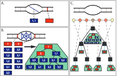
We let each move contain a reference to the loop(s) it affects (Figure 5.2A), as well as

an index to the bases within the loop, such that we can uniquely identify the structural

change that should be performed if this move is chosen. This reference allows us to quickly

find the affected loop(s) once a move is chosen. We then collect all the moves which affect a

particular loop and store them in a container associated with the loop (Figure 5.2B). This

allows us to quickly access all the moves associated with a loop whose structure is being

modified by the current move. We should note that since deletion moves by nature affect

the two loops adjacent to the base pair being deletion, they must necessarily show up in the

available moves for either loop. This is handled by including a copy of the deletion move in

each loop’s moves, and halving the rate at which each occurs.

Finally, since this method of move storage is not a global structure, we add a final layer

of complexity on top, so that we can easily access all the moves available from the current

state without needing to traverse the loop graph. This is as simple as storing each loop’s

(33)

complex’s available moves as shown in figure 5.2C.

A.

B.

1, 1 1,1 1,2 1,3 2,1 2,2 2,3 3,1 3,2 3,3 1 2 1,1 1,2

1,3 2,1 2,2

2,3 3,1 3,2

3,3 2 1

C.

1,1 1,2

1,3 2,1 2,2

2,3 3,1 3,2

3,3 2

1

Figure 5.2: (A) Creation moves (blue line) and deletion moves (red highlight) are repre-sented here by rectangles. Either type of move is associated with a particular loop, and has indices to designate which bases within the loop are affected. (B) All possible moves which affect the interior loop in the center of the structure. These are then arranged into a tree (green area), which can be used to quickly choose a move. (C) Each loop in the loop graph then has a tree of moves that affect it, and we can arrange these into another tree (black boxes), each node of which is associated with a particular loop (dashed line) and thus a tree of moves (blue line). This resulting tree then contains all the moves available in the complex.

5.2

Algorithms

The second main piece of the simulator is the algorithms that control the individual steps of

the simulator. The algorithm implementing the Markov process simulation closely follows

the Gillespie algorithm[8] in structure:

1. Initialization: Generate the initial loop graph representing the input state, and

com-pute the possible transitions.

2. Stochastic Step: Generate random numbers to determine the next transition (5.2.1),

(34)

3. Update: Change the current loop graph to reflect the chosen move (5.2.2). Recompute

the available transitions from the new state (5.2.3). Update the current time using

the time interval in the previous step.

4. Check Stopping Conditions: check if we are at some predetermined stopping condition

(such as a maximum amount of simulated time) and stop if it is met. Otherwise,

go back to step 2. These stopping conditions and other considerations relating to

providing output are discussed further in section 6.

The striking difference between this structure and the Gillespie algorithm is the

neces-sity of recomputing the possible transitions from the current state at every step, and the

complexity of that recalculation. Since we are dealing with an exponential state space we

have no hope of storing all possible transitions between any possible pair of states, and

instead must look at the transitions that occur only around the current state. Our

exam-ination of the key algorithms must include an analysis of their efficiency, so we define the

key terms here:

1. N, the total length of the input’s sequence(s).

2. T, the total amount of simulation time for each Monte Carlo trajectory.

3. J, the number of nodes in the loop graph of the current state. At worst case, this is

O(N), which occurs in highly structured configurations, like a full duplex.

4. K, the largest number of unpaired bases occuring in any loop in the current state. At

worst case, this is exactlyN, but on average it is typically much smaller.

5. L, the current number of complexes in the system. At worst this could beO(N), but

in practice the number of complexes is much fewer.

5.2.1 Move Selection

First let’s look at the unimolecular moves in the system. The tree-based data structure

containing the unimolecular moves leads to a simple choice algorithm that uses the generated

random number to make a decision at each level of the tree based on the relative rates of

the moves in each branch. We have two levels of tree to perform the choice on, the first

(35)

for a particular loop, and the second having at mostO(K2) nodes (the worst case number of

moves possible within a single loop). Thus our selection algorithm for unimolecular moves

takes O(log(J) + log(K)) time to arrive at a final decision.

What about the moves that take place between two different complexes? With our

method of assigning rates for these moves, we know that regardless of the resulting structure,

all possible moves of this type must occur at the same rate. Thus the main problem is

knowing how many such moves exist and then efficiently selecting one.

How many such moves exist? This is a straightforward calculation: for each complex

microstate in the system, we count the number of A, G, C and T bases present in open

loops within the complex. For the sake of example, let’s call these quantitiescA, cG, cC, cT

for a complex microstate c. Let’s also define the total number of each base in the system

as follows: Atotal =Pc∈scA, etc, where s in the system microstate we are computing the

moves for. We can now compute how many moves there are where (for example) anAbase

in complex c becomes paired with a T base in any other complex: cA∗(Ttotal−cT), that

is, the number ofAbases withinc multiplied by the number ofT bases present in all other

complexes in the system. So the number of moves betweencand any other complex in the

system is thencA∗(Ttotal−cT) +cG∗(Ctotal−cC) +cC∗(Gtotal−cG) +cT∗(Atotal−cA) and

if we allow GT pairs, there are two additional terms with the same form. Summing over

this quantity for eachc∈swe then get 2 times the total number of bimolecular moves (and

in fact we can eliminate the redundency by using the total open loop bases in complexes

“after”cin our data structure, rather than the total open loop bases in all complexes other

thanc). Since we do this in an algorithmic manner, it is straightforward to uniquely identify

any particular move we need by simply following this counting process in reverse.

What is the time complexity for this bimolecular move choice? It is straightforward

to see that calculating the total bimolecular move rate is O(L) (recall L is the number of

complexes within the system). Slightly more complex is choosing the bimolecular move,

which must also beO(L), as it takes 2 traversals through the list of complexes to determine

the pair of reacting complexes in the bimolecular step. We note that for typical L and

bimolecular reaction rates (e.g. typical strand concentrations which set our ∆Gvolume) this

quantity is quite small relative to that for the unimolecular reactions.

Our move choice algorithm can now be summed up as follows: given our random choice,

(36)

first step) or unimolecular (thus one of the ones stored in the tree). If it’s bimolecular,

reverse the counting process using the random number to pick the unique combination of

open loops and bases involved in the bimolecular step. If it’s a unimolecular step, pick a

move out of the trees of moves for each complex in the system as discussed above.

5.2.2 Move Update

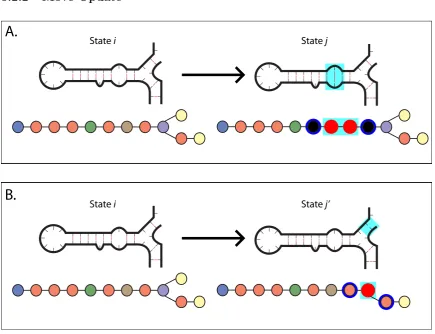
A.

_State_i _State_j

B.

_State_i _State_j’

Figure 5.3: Moves of varying types which take current stateito statej. The changed region is highlighted incyan. Loops that are injbut notiare highlighted in red (in the loop graph) and must be created and have their moves generated. Loops shown highlighted in blue have had an adjacent loop change, and thus must have their deletion moves recalculated. (A) A creation move. (B) A deletion move.

Once a move has been chosen, we must update the loop graph to reflect the new state.

This is a straightforward substitution: for a creation move, which affects a single loop, we

must create the resulting pair of loops which replace the affected loop and update the graph

connections appropriately (Figure 5.3A). Similarly, for a deletion move, which affects two

loops, we must create the single loop that results from joining the two affected loops, and

(37)

The computationally intensive part for this algorithm lies in the updating of the tree

structure containing all the moves. We must remove the moves which involved the affected

loops from the container, a process that takesO(log(J)) time (assuming we implement tree

deletions efficiently), generate the moves which correspond to the new loops (Section 5.2.3),

and add these moves into the global move structure, which also takesO(log(J)) time.

5.2.3 Move Generation

The creation and deletion moves must be generated for each new loop created by the move

update algorithm, and we must update the deletion moves for each loop adjacent to an

affected loop in the move update algorithm. The number of deletion moves which must be

recalculated is fixed, though at worst case is linear in N, and so we will concern ourselves

with the (typically) greater quantity of creation moves which need to be generated for the

new loops.

For all types of loops, we can generate the creation moves by testing all possible

combi-nations of two unpaired bases within the loop, tossing out those combicombi-nations which are too

close together (and thus could not form even a hairpin, which requires at least three bases

within the hairpin), and those for which the bases could not actually pair (for example, a

T–T pairing). An example of this is shown for a simple interior loop, in figure 5.4. The

remaining combinations are all valid, and we must compute the energy of the loops which

would result if the base pair were formed, in order to compute the rate using one of the

kinetic rate methods (Section 4.5). This means we need to check O(L2_{) possible moves}

and do two loop energy computations for each. At worst case, that isO(N2) energy

com-putations in this step, and so the efficiency of performing an energy computation becomes

vitally important.

Once we have generated these moves we must collect them into a tree which represents

the new loop’s available moves. This can be handled in a linear fashion in the number of

moves with a simple tree creation algorithm, and thus it is in the same order as the number

(38)

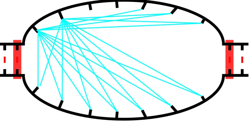
Figure 5.4: A interior loop, with all theoretically possible creation moves for the first two bases on the top strand shown as cyanlines, and all possible deletion moves shown as red boxes. Note that for each creation move shown here, we must check whether the bases could actually pair, and only then continue with the energy computations to determine the rate of the move.

5.2.4 Energy Computation

It is in the energy computation that our loop graph representation of the complex microstate

shines, as the basic operation required for each possible move in the move generation step

is computing the difference of energies between the affected loop(s) that would be present

after the move and those present beforehand.

For all loop types except open loops and multiloops, computing the loop energy is as

simple as looking up the sequence information (base pairs and adjacent bases) and loop

sizes in a table [16, 27], and is a constant-time lookup. For open loops and multiloops, this

computation is linear in the number of adjacent helices (e.g. adjacent nodes in the loop

graph) if we are using an optional configuration of the energy model which adds energies

that come from bases adjacent to the base pairs within the loop (called the “dangles”

option). Theoretically we could have an open loop or multiloop that is adjacent to O(N)

other nodes in the loop graph, but this is an extraordinarily unlikely situation and present

only with particular energy model options, so we will consider the energy computation step

(39)

5.3

Analysis

Now that we have examined each algorithm needed to perform a single step of the

stochas-tic simulation, we can derive the worst-case time. First, recall that J is the number

of nodes in the loop graph, K is the largest number of unpaired bases in a loop, L is

the number of complexes in the system and N is the total length of strands in the

sys-tem. The move selection algorithm is O(log(J) + log(K) +L) = O(N), move update is

O(log(J)) =O(log(N)), and move generation is O(N2∗O(1)), where energy computation

is theO(1) term. These algorithms are done in sequence and thus their times are additive:

O(N) +O(log(N)) +O(N2) =O(N2). Thus our worst case time for a singleMarkov step is quadratic in the number of bases in our structure.

However, one step does not a kinetic trajectory make. We are attempting to simulate

for a fixed amount of time T, as mentioned before, and so we must compute the expected

number of steps needed to reach this time. Since the distribution on the time interval ∆t

between steps is an exponential distribution with rate parameter R, which is the total rate

of all moves in the current state, we know that the expected ∆t= 1/R. However, this still

leaves us needing to approximateR in order to compute the needed amount of time for an

entire trajectory. To make a worst case estimate, we must use the largest R that occurs

in any given trajectory, as this provides the lower bound on the mean of the smallest time

step ∆tin that trajectory. However, the relative rates of favorable moves tends to be highly

dependent on the rate method used: the Kawasaki method can have very large rates for

a single move, while the Metropolis method has a maximum rate for any move, and the

Entropy/Enthalpy method is also bounded in this manner as all moves have to overcome

an energy barrier.

We thus make an average case estimate for the the total rate R, based on the number

of “favorable” moves that typically have the largest rates. While a “favorable” move is

merely one where the ∆G is negative (thus it results in an energetically more favorable

state) or one which uses the maximum rate (for non-Kawasaki methods), the actual rate

for these moves depends on the model chosen. The key question is whether we can come up

with an average situation where there areO(N2) favorable moves or ifO(N) is more likely.

What types of secondary structures give rise to quadratic numbers of moves? They are all

(40)

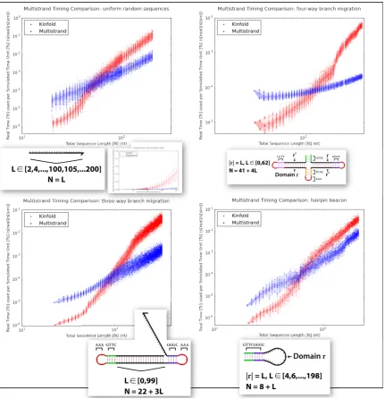
N = L

L ∈ [2,4,...,100,105,...200]

AAA GTTC GGGC

TCAC CCTT

Domain r r r’ r’

N = 22 + 3L L ∈ [0,99]

AAA

AAAGTTC GGGC GTTCGGGC

Domain r

Figure 5.5: Comparison of real time used per simulated time unit between Multistrand and Kinfold 1.0, for four different single stranded systems with varying total length. All plots are log/log except for the inset, which is a linear/linear plot of the same data is in the uniform random sequence plot. The density of test cases is shown using overlaid regions of varying intensity. From lightest to darkest, these correspond to 80%, 40% and 10% of the test cases being within the region.

or open loop. These creation moves are generally unfavorable, except for the small number

that lead to new stack loops. Thus we do not expect there to be a quadratic number of

favorable moves. A linear number is much more likely: a long duplex region could reach a

(41)

we make the (weak) argument that a good average case is that the average rate is at worst

O(N).

From this estimate for the average rate, we conclude that each step would have an

expected (lower bound) ∆t = 1/N, and thus to simulate for time T we would need

T /(1/N) = T ∗N steps, and thus O(T ∗N3) time to simulate a single trajectory. Since

this is the worst case behavior, it is fairly difficult to show this with actual simulation data,

so instead we present a comprehensive comparison with the original Kinfold for a variety

of test systems (Figure 5.5), noting that the resulting slopes on the log/log plots lie easily

(42)

Chapter 6

Multistrand : Output and Analysis

We have now presented the models and algorithms that form the continuous time Markov

process simulator. Now we move on to discuss the most important part of the simulator

from a user’s perspective: the huge volume of data produced by the simulation, and methods

for processing that data into useful information for analyzing the simulated system.

How much data are we talking about here? Following the discussion in the previous

chapter, we expect an average of O(N) moves per time unit simulated. This doesn’t tell

us much about the actual amount of data, only that we expect it to not change drastically

for different size input systems. In practice this amount can be quite large, even for simple

systems: for a simple 25 base hairpin sequence (similar to Fig 5.5D), it takes 4,000,000

Markov steps to simulate 1s of real time. For an even larger system, such as a 4-way

branch migration system (Fig 5.5C) with 108 total bases, simulating 1s of real time takes

14,000,000 Markov steps.

What can we do with all the data produced by the simulator? In the following sections

we discuss several different processing methods.

6.1

Trajectory Mode

This full trajectory information can be useful to the user in several ways: finding kinetic

traps in the system, visualizing a kinetic pathway, or as raw data to be passed to another

analysis tool.

Trajectory mode is Multistrand’s simplest output mode. The data produced by this

mode is a trajectory through the secondary structure state space. While many trajectories

(43)

we are only concerned with a single trajectory. Similarly, these trajectories are infinite

but unfortunately our computers have only a finite amount of storage so we must cut the

trajectory off at some point.

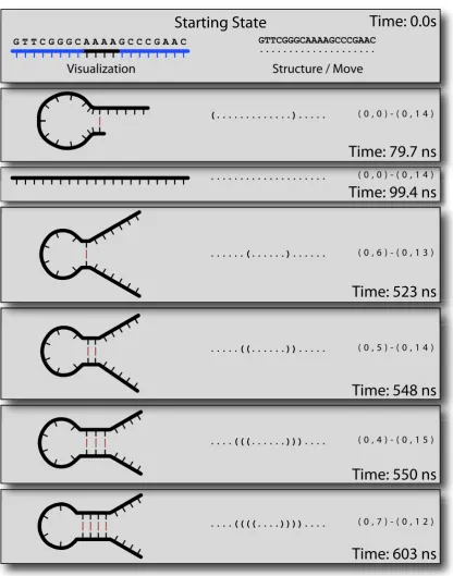
Time: 603 ns

( 0 , 7 ) - ( 0 , 1 2 ) ....((((....))))....

Time: 550 ns

( 0 , 4 ) - ( 0 , 1 5 ) ....(((...)))....

Time: 548 ns

( 0 , 5 ) - ( 0 , 1 4 ) ...((...))...

Time: 523 ns

( 0 , 6 ) - ( 0 , 1 3 ) ...(...)...

Time: 99.4 ns

... ( 0 , 0 ) - ( 0 , 1 4 ) ... ( 0 , 0 ) - ( 0 , 1 4 ) ( 0 , 0 ) - ( 0 , 1 4 )

Time: 79.7 ns

(...)...

GTTCGGGCAAAAGCCCGAAC ...

Starting State

Time: 0.0s

Structure / Move

Visualization

G T T C G G G C A A A A G C C C G A A C

Figure 6.1: Trajectory Data

(44)

microstate, and tis the time in the simulation at which that state is reached. We call this

time thesimulation time, as opposed to thewall clock time, the real world time it has taken

to simulate the trajectory up to that point. There are many different ways to represent a

trajectory, as shown in Figure 6.1.

For practical reasons, we set up conditions to stop the simulation so that our trajectories

are finite. There are two basic stop conditions that can be used, and the system stops when

any condition is met:

1. Maximum simulation time. We set a maximum simulation time t0 for a trajectory,

and stop when the current simulation state (s, t) hast > t0. Note that the state (s, t)

which caused the stopping condition to be met is not included in the trajectory, as it

is different from the state at timet0.

2. Stop state. Given a system microstate s0, we stop the trajectory when the current

simulation state (s, t) has s = s0. This type of stopping condition can be specified

multiple times, with a new system microstate s0 each time; the simulation will stop

when any of the provided microstates is reached.

We will now use an example to show how trajectory mode can be used to compare two

different sequence designs for a particular system. The system is a straightforward

three-way branch migration with three strands, with a six base toehold region and twenty base

branch migration region, shown below (Fig 6.2).

. . .

Start State

Branch Migration

Disassociation

(45)

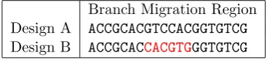
The simulation is started in the shownStart Stateusing a toehold sequence of GTGGGT and a differing branch migration region for which we use the designs in Table 6.1. We then

start trajectory mode for each design, with a stop condition of 0.05 s of simulation time,

and save the resulting trajectories.

Branch Migration Region Design A ACCGCACGTCCACGGTGTCG Design B ACCGCACCACGTGGGTGTCG

Table 6.1: Two different branch migration sequences

Rather than spam the interested reader with several thousand pages of trajectory

print-outs, since there are 5∗106states in a 0.05 s trajectory for this system, we instead highlight

one revealing section in each design’s trajectory. Let us look at the state the trajectory is

in after 0.01 s of simulation time, shown below in Figure 6.3 using a visual representation.

Design A

Design B

Figure 6.3: Structure after 0.01 s simulation time for two different sequence designs.

What happened? It appears that sequence designAhas a structure that can form before

the branch migration process initiates, that contains a hairpin in the single stranded branch

migration region. Does this structure prevent the branch migration from completing? In

the long run it shouldn’t, as the equilibrium structure remains unchanged, but if we look

at the final state in each trajectory (Figure 6.4), we see that design B has completed the

process in 0.05 s of simulation time and indeed was complete at 0.01 s, whereAis still stuck

in that offending structure after the same amount of time. So for these specific trajectories,

it’s certainly slowing down the branch migration process.

Did this structure only appear because we were unlucky in the trajectory for design A?

We could try running several more trajectories and seeing whether it appears in all or most

of them, but a more complete answer is better handled using a different simulation mode,

such as the first passage time mode discussed in Section 6.4.

A better type of question for trajectory mode is “How did this kinetic trap form?”. In

(46)

Design A

Design B

Figure 6.4: Final structure (0.05 s simulation time) for the two different sequence designs from Table 6.1. Branch migration regions: Design A: ACCGCACGTCCACGGTGTCG, Design B: ACCGCACCACGTGGGTGTCG.

microstates that lead to the first time the hairpin structure forms. This example has a

straightforward answ