Mean-Dependent Spatial Prediction Methods with Applications to Materials Sciences.

(1)

ABSTRACT

PETERSON, GEOFFREY COLIN LEE. Mean-Dependent Spatial Prediction Methods with Applications to Materials Sciences. (Under the direction of Dr. Brian Reich and Dr. Joseph Guinness.)

In this work, we explore spatial statistical models and their potential uses in materials

science, with particular emphasis on mean-dependent covariance structures. Materials science, which is the study and design of new solid materials, is a field ripe with complex data that

requires sophisticated statistical analysis. We investigate two important materials science data

applications: molecular dynamics simulations and crystallography diffraction analysis.

For the molecular dynamics simulations, computer simulations of the three-dimensional

atomic structures of materials explore how defects arise under simulated stresses. To overcome

the extreme computational burden of these simulations, we develop a spatial statistical model that emulates the final output of these computationally-intensive simulations. In a comparison

of multiple spatial regression methods, we find that principal component analysis best predicts

defects in the atomic structure.

For the crystallography analysis, radiation diffraction patterns are used to identify the

crys-tal lattice properties of a solid material. We investigate a statistical method of fusing the

multiple diffraction data sources to estimate the crystallographic parameters. We determine that variable weighting of the data sources significantly improves the accuracy of the estimates,

particularly when parts of the diffraction sources were unreliable due to data corruption.

Finally, as an extension of methods used in the materials sciences analyses, we develop a nonstationary spatial model where the covariance structure is indexed by the mean. Through

a simulation study, we explore the inferential and predictive capabilities of the model, showing

that it significantly improves upon a stationary spatial model under various circumstances. We then demonstrate these methods on daily precipitation data in Puerto Rico to show how they

(2)

(3)

Mean-Dependent Spatial Prediction Methods with Applications to Materials Sciences

by

Geoffrey Colin Lee Peterson

A dissertation submitted to the Graduate Faculty of North Carolina State University

in partial fulfillment of the requirements for the Degree of

Doctor of Philosophy

Statistics

Raleigh, North Carolina

2016

APPROVED BY:

Dr. Donald Brenner Dr. Peter Bloomfield

Dr. Brian Reich

Co-chair of Advisory Committee

(4)

ACKNOWLEDGEMENTS

First and foremost, I would like to thank Dr. Brian Reich and Dr. Joseph Guinness as my advisors. Your guidance, support, and vast knowledge have helped brought this thesis to fruition.

Next, I would like to acknowledge our many collaborators from North Carolina State Uni-versity. Thank you to Dr. Don Brenner and Dong Li from the Department of Materials Sciences,

who generated the molecular dynamics simulation data. Thank you to Dr. Chris Fancher and

Dr. Jacob Jones from the Department of Materials Sciences and Engineering, who advised us on the crystallography analysis. Thank you to Dr. Adam Terando from the Department of Ecology,

who advised on the Puerto Rico precipitation analysis.

I would also like to acknowledge some of the many friends who have provided me with extensive personal support. In no particular order, thank you to Victoria Weber, Benjamin

Burner, Christropher Krut, Keith Shusterman, Timothy Scheisswohl, Kevin Garofalo and The

Raleigh Social Club, the friendly staff of Cup-A-Joes, and everyone else who made me laugh and smile along the way. And thank you to Adrienne Mazzo, who has made my life so bright,

beautiful, and full of joy.

Of course, I would not be anywhere without the love and support of my family. Thank you to my oldest brother Luc, for being a fantastic role model. Thank you to my brother Carl, for

being a constant source of diversion. Thank you to Annika, my dear sister and fellow

brown-eyed Lee, for being one of my best friends in the world. Thank you to my awesome sister-in-law Meghan and my beautiful niece Madeline, for growing the amount of love in my family. Thank

you to my grandmother Shirley, my aunts DeeAnn, Lori, Ann, and Pat, my uncles Bob, Brian,

and Drew, and my cousins Josh, Erin, Chris, Nick, and Drew.

Finally, thank you to my parents, Lee and Mary. You have given me everything in this

world, and I would not have been able to accomplish anything without your love and support.

I could not be more happy and proud to be your son.

(5)

DEDICATION

To the loving memories of my grandparents, Jay Peterson and Daisy Lee Shores.

(6)

TABLE OF CONTENTS

LIST OF TABLES . . . vi

LIST OF FIGURES . . . vii

Chapter 1 Spatial prediction of crystalline defects observed in molecular dy-namic simulations of plastic damage . . . 1

1.1 Introduction . . . 1

1.2 Data simulation and processing . . . 4

1.2.1 Simulation generation . . . 4

1.2.2 Quantifying materials defects . . . 5

1.2.3 Coarse graining . . . 6

1.3 Model description . . . 6

1.3.1 Prior Distributions . . . 7

1.3.2 Spatial Projections . . . 8

1.3.3 Basis Functions of Input Space . . . 12

1.4 Computing Details . . . 13

1.4.1 Reducing dimension to improve computation time . . . 14

1.4.2 Prediction Distribution . . . 15

1.5 Results . . . 15

1.6 Conclusion . . . 23

Chapter 2 Bayesian estimation of crystallographic parameters through weighted fusion of radiation diffraction data . . . 24

2.2 Statistical Model . . . 26

2.3 Computational Details for Parameter Estimation . . . 28

2.3.1 Background and Precision Parameters . . . 28

2.3.2 Crystallographic Parameters . . . 29

2.4 Simulation Study . . . 29

2.4.1 Data Generation . . . 29

2.4.2 Results and Discussion . . . 32

Chapter 3 Mean-dependent nonstationary spatial models . . . 43

3.2 Nonstationary spatial model from conditionally stationary regimes . . . 45

3.3 Computation . . . 46

3.3.1 The Stationary Model . . . 47

3.3.2 The Nonstationary Model . . . 47

3.4 Evaluation of models . . . 47

3.4.1 Test for Nonstationarity . . . 48

3.4.2 Prediction Distribution . . . 48

3.5 Simulation study . . . 49

(7)

3.5.1 Simulated data generation . . . 49

3.5.2 Type I error rate for nonstationarity test . . . 50

3.5.3 Parameter estimation accuracy . . . 50

3.5.4 Prediction distribution accuracy . . . 51

3.6 Data application: Precipitation data in Puerto Rico . . . 51

3.6.1 May 2013 data . . . 52

3.6.2 January 2013 data . . . 53

BIBLIOGRAPHY . . . 71

APPENDICES . . . 78

Appendix A Matrix Normal Distribution . . . 79

Appendix B Derivation of Posterior Distributions . . . 81

B.1 Posterior ofB∗ . . . 81

B.2 Posterior ofG. . . 82

B.3 Posterior ofΣ . . . 82

B.4 Posterior ofτ . . . 83

B.5 Posterior ofρ for CAR Model . . . 83

B.6 Posterior ofqii for DWT Model . . . 84

Appendix C Cross-validation Results . . . 85

Appendix D Covariance parameter MSEs . . . 88

(8)

LIST OF TABLES

Table 1.1 Cross-validation results, averaged over all prediction angles (10 - 80) . . . . 16

Table 1.2 Cross-validation results, averaged over interpolation angles (20 - 70) . . . . 16

Table 2.1 Accuracy of crystallographic parameters (I0,λ, 2θ0) . . . 38

Table 2.2 Accuracy of crystallographic parameters (U,V,W) . . . 39

Table 2.3 Coverage of crystallographic parameters (I0,λ, 2θ0) . . . 40

Table 2.4 Coverage of crystallographic parameters (U,V,W) . . . 41

Table 3.1 Estimation Accuracy for Simulated Data . . . 58

Table 3.2 Mean computation time (in seconds) for simulated data. . . 58

Table 3.3 Evaluation of Prediction Distributions for Simulated Data . . . 59

Table 3.4 Covariance parameter estimates for Puerto Rico precipitation data . . . . 61

Table 3.5 Five-fold cross-validation results for Puerto Rico precipitation data . . . . 62

(9)

LIST OF FIGURES

Figure 1.1 Example output for a molecular dynamics simulation . . . 3

Figure 1.2 Cross-validation results across all tilt tension angles. . . 17

Figure 1.3 Predictions from cross-validation for tilt angle 10 . . . 19

Figure 1.6 Predictive accuracy dimension reduction results for CAR and DWT models 22 Figure 2.1 True X-ray F1(2θ) and neutron F2(2θ) signals . . . 30

Figure 2.2 Absolute error between fitted and true X-ray signal for simulated data sets. 33 Figure 2.3 Absolute error between fitted and true neutron signal for simulated data sets. . . 34

Figure 2.4 Fitted X-ray background scattering for simulated data sets. . . 35

Figure 2.5 Fitted neutron background scattering for simulated data sets. . . 36

Figure 2.6 Fitted variable weighting functions for simulated data sets. . . 37

Figure 3.1 Means and standard deviations for Puerto Rico data . . . 55

Figure 3.2 Daily mean and max values for Puerto Rico data . . . 55

Figure 3.3 Maps of observed values for Puerto Rico data . . . 56

Figure 3.4 Longitude, latitude, and elevation across the island of Puerto Rico. . . 56

Figure 3.5 Simulated stationary and nonstationary data for two sites . . . 57

Figure 3.6 Type I error rate for nonstationarity test at 5% significance level . . . 60

Figure 3.7 Empirical correlograms for January 2013 and May 2013. . . 60

Figure 3.8 Fitted correlation functions for May 2013 . . . 63

Figure 3.9 Fitted correlation functions for January 2013 . . . 64 Figure 3.10 Predictions and standard deviations for 9 May 2013 usingp= 2 predictors. 65 Figure 3.11 Predictions and standard deviations for 9 May 2013 usingp= 4 predictors. 66 Figure 3.12 Predictions and standard deviations for 9 May 2013 usingp= 7 predictors. 67 Figure 3.13 Predictions and standard deviations for 26 Jan. 2013 usingp= 2 predictors. 68 Figure 3.14 Predictions and standard deviations for 26 Jan. 2013 usingp= 4 predictors. 69 Figure 3.15 Predictions and standard deviations for 26 Jan. 2013 usingp= 7 predictors. 70

(10)

Chapter 1

Spatial prediction of crystalline

defects observed in molecular

dynamic simulations of plastic

damage

Molecular dynamic computer simulation is an essential tool in materials science to study atomic properties of materials in extreme environments and guide development of new materials. We

propose a statistical analysis to emulate simulation output with the ultimate goal of efficiently

approximating the computationally-intensive simulation. We compare several spatial regression approaches including conditional autoregression (CAR), discrete wavelets transform (DWT),

and principal components analysis (PCA). The methods are applied to simulation of copper atoms with twin wall and dislocation loop defects, under varying tilt tension angles. We find

that CAR and DWT yield accurate results but fail to capture extreme defects, yet PCA better

captures defect structure.

1.1 Introduction

The permanent deformation of a crystalline material is typically accompanied by the creation

of defects that disturb the lattice structure. These defects can be in the form of partial planes of atoms (dislocations), atoms missing from lattice sites or in positions between sites (vacancies

and interstitials, respectively), regions of missing atoms (voids), boundaries across which the

(11)

lattice orientation changes (twins and grain boundaries), and regions in which the atoms are disordered (amorphous regions) [FA77].

Traditional modeling of plastic damage in metals involves numerically solving continuum

constitutive equations that relate structure, stress, strain and mechanical response. In recent decades, however, atom-scale approaches have started to play a larger role in modeling plastic

damage [Lu15]. In molecular dynamics simulations, for example, trajectories of individual atoms

are followed in time from an initial configuration by numerically integrating classical equations of motion that are coupled through a prescribed set of inter-atomic forces. Examination of the

trajectories, typically either through animations of the atom motion or by more quantitative

analyses, yields information about structures and their formation mechanisms as simulation conditions evolve. To study plastic deformation in a crystalline metal, for example, the motion

of collections of atoms can be followed as a system is strained.

The computational costs of a molecular dynamics simulation increase with an increasing number of atoms and with the length of time over which the atom motion is simulated. Because

of this, with current computing capabilities, simulations of plastic damage in crystals are typi-cally restricted to sub-micron length scales and sub-microsecond time scales, respectively, which

are far below practical engineering scales. Two of the leading challenges to molecular dynamics

simulations of this type are therefore making the simulations more efficient, and bridging de-fect formation mechanisms determined at the atomic scale with continuum, engineering-scale

constitutive relations [Bre13; MT09]. The results reported in this paper are a first step

to-ward exploring a unique response to these challenges in which coarse-grained representations of atomic configurations that evolve during plastic strain are connected through a statistical

model that is trained from a subset of fully atomistic simulations. Building prediction models

from computer simulation output is the focus of surrogate modeling [Sac89; Ken02], computer emulation [Bay07; Rou08], and meta-modeling [Che11; Wan14], but rarely have these methods

been applied in this manner to molecular dynamics.

To make a statistical analysis feasible, defect configurations from simulations with several hundreds of thousands of atoms are summarized by three-dimensional arrays of voxels that

contain information regarding defect types and densities (Figure 1.1). Our objective is to build

a statistical model to predict voxel profiles that correspond to atomic defect densities that would arise from the corresponding molecular dynamics simulation. We treat each array of

voxels as the functional response to the simulation conditionals, which frames the analysis

as a function-on-scalars regression problem. Methods for this kind of functional data analysis (FDA) have been explored at length in the past several years. General FDA methods have

been explored at length in [SR05] and [HK12], with typical approaches being either functional

(12)

Figure 1.1 Example output for a molecular dynamics simulation

Left: values for individual atoms, thresholded at 1 to indicate a molecular deformation around the atom. Right: 16×16×16 array of voxels with mean values, thresholded at 0 to indicate a molecular deformation within the voxel. Thresholds were chosen to clearly depict only poten-tially defective atoms/voxels that would be obscured by the clearly non-defective parts of the solid.

(13)

linear models [Cra09; He10], functional principal component analysis (FPCA) [Di09; Gre11], or nonparametric FDA [FV06]. FDA becomes more intricate when handling dependent functional

responses [Kok12], but a general approach is a functional additive mixed model [Sch14], which

flexibly accounts for a variety of correlation structures between functional responses. In our case, the functional response exhibits spatial dependence, which has been explored in [Del10], [Sta10],

and [Ram11]. Modeling this spatially-dependent functional response requires computationally

efficient representation of the spatial patterns to isolate those patterns that vary with functional factors.

In this paper, we explore statistical models to emulate results for molecular simulations of

defects created in strained metals. Our objective is to present and compare several approaches to this problem, evaluate the feasibility of applying statistical methods for this problem, and

offer recommendations for future development. We present a general approach to accommodate

both spatial variation across voxels and variation within a voxel across simulated conditions. While molecular dynamics includes temporal variation, we will focus on predicting the final state

of the simulation from more generalized conditions. For computational simplicity and ease of interpretation, we assume separability between the spatial variation and the simulation variation

[Gal94; NR01]. We project the simulation output into a spatially uncorrelated space using a

variety of spatial dependence structures: conditional autoregression (CAR) [Bes74], discrete wavelet transforms (DWT) [Mal89], and principal component analysis (PCA) [Hot33]. Variation

across design conditions is explained using semiparametric regression methods including Fourier

and Bernstein basis expansions. We utilize the matrix normal distribution [Daw81] to achieve a computationally efficient Markov chain Monte Carlo algorithm to fit the model. We apply the

methods to an atomic simulation of copper, evaluate the performance of the statistical model,

and provide recommendations for future research in this direction.

1.2 Data simulation and processing

1.2.1 Simulation generation

In molecular dynamics simulations atom trajectories are followed by numerically integrating

classical equations of motion that are coupled through a prescribed set of inter-atomic forces.

The simulations reported here were carried out using the LAMMPS software [Pli95], with interatomic forces from a many-body embedded-atom method potential for copper [Mis01].

The systems contained about 500,000 atoms in a periodic box with sides of roughly 1.6·10−8

meters; the numerical integration used a time step of 10−15 seconds. Initial atomic positions

(14)

for the grain boundaries were generated from two face-centered cubic lattices that were rotated by angles±θ along the<100>direction. The two lattices were then cut so that with periodic boundaries they met at two symmetric tilt grain boundaries in the direction perpendicular to the

applied strain, and so that the system satisfied the periodic boundaries in all three directions. Atoms were then removed that were less than 0.2 nm apart along the grain boundaries (for

reference the copper-copper near-neighbor distance is 0.254 nm) . In addition to the set of

symmetric tilt grain boundaries, separate systems with dislocation loops were also generated by removing slices of copper atoms from an ideal lattice. After the initial atomic configurations

were generated, the atom positions for each system were relaxed to minimize the potential

energy. This was followed by a constant-volume anneal at 300K for 100 ps.

To generate plastic damage, the systems were strained along the direction normal to the

grain boundaries (with no tilt this is the <100> direction) by scaling atom positions and the box length by a constant engineering strain up to a total strain of 0.1 over 100,000 time steps. This extremely rapid strain rate is a result of the computational limitations on system size and

time scale that are inherent to molecular dynamics simulations. While comparison to typical strain rates, which are order of magnitude slower, may be inappropriate, this high strain rate

is acceptable for the present study because of our goal of a statistical description of molecular

simulation results. To eliminate noise in the data, the atomic measures, such as the centro-symmetry parameter described in Section 1.2.2, were averaged over each 100 time steps during

the simulations.

1.2.2 Quantifying materials defects

While other atomic measures (e.g. common neighbor analysis, virial stress, and potential and kinetic energy) are possible defect summaries, we focus on the centro-symmetry parameter for

each atom,

CSP = 6

X

i=1

|Ri+Ri+6|2, (1.1)

where theRiterms represent directional vectors to the twelve nearest neighboring atoms, paired

such thatRi andRi+6have opposite directions [Kel98]. Compared to the other measures, CSP most efficiently measures the strength of defects in the crystal lattice. For a face-centered cubic lattice (which is the stable, ideal structure for copper), the ideal CSP value would be zero for

non-defective atoms and higher values for different defect types. Local fluctuations in atomic

structure due to vibrations in a molecular dynamics simulation can change these values, but the changes are sufficiently small that different types of defects can be clearly discerned. To eliminate

(15)

noise in the data from the simulation, the CSP values used in the analysis were averaged over each 100 time steps during the simulations. For this study, a logarithmic transform of the CSP

was used to allow for the normality assumptions made in Section 1.3.

1.2.3 Coarse graining

Coarse graining reduces the size of the data from several hundred thousand particles to a more manageable size. The spatial domain is divided into a cubic array of cells, or “voxels,” and

summary values are obtained for each cell. Coarse graining has often been used in molecular dynamics studies to simplify computation, such as polymer simulation [MP02] and biomolecular

systems [IV05]. Voxel-wise analysis is also used in medical imaging, particularly functional MRI

data [Wor02; Woo09], and uses projection methods to identify independent structures in the images [Lee11; Kaw12]. The number of grid cells should be large enough to capture important

structural features but small enough to permit efficient computing. Based on our exploratory

analysis and computing limitations discussed in Section 1.3.2.2, a 16 x 16 x 16 cubic grid sufficiently captured important spatial features. As the summary response, we use the mean

log-CSP for all particles in the voxel. Therefore the results of each simulation are represented

by n= 163 observations in a 3-D array, as seen in Figure 1.1. Other data summaries, such as the mean CSP, were attempted during the analysis but did not significantly affect results.

1.3 Model description

Let Y(s|θ) be the response in spatial cell s of the solid when the simulator is evaluated at L design features θ= (θ1, . . . , θL) . In our example, the L= 2 input values are tilt tension angle

(continuous) and the presence of a dislocation loop (binary) as discussed in Section 1.3.3. The responses are modeled using separable functions

Y(s|θ) =

p

X

k=1

βk(s)φk(θ) +e(s|θ), (1.2)

whereβk(s) are spatially-dependent coefficients,φk(θ) are fixed functions of inputs, ande(s|θ)

is the error. Therefore, variation in the response across design factors θ is regressed onto p basis functionsφk(θ), and the regression varies across the locationssvia the spatial coefficients

βk(s).

In vector form, the responses at n spatial locations s1, . . . ,sn for a given input θj are

expressed asYj = [Y(s1|θj), . . . , Y(sn|θj)]T. The simulator is evaluated atminputsθ1, . . . ,θm

(16)

to create the response matrix Y= [Y1. . .Ym]. The statistical model in (1.2) is written as

Y

n×m=nB×ppA×m+nE×m, (1.3)

where the elements ofB,A, andE are βk(si), φk(θj), ande(si|θj), respectively.

1.3.1 Prior Distributions

We use the matrix normal distribution [Daw81] to account for the dependence between and

within the rows and columns of the mean parameters B and errors E. See Appendix A for a full description of this distribution. The major assumption here is that the spatial covariance is separable from the design factor covariance,

Cov [e(s1|θ1), e(s2|θ2)] = CS(s1,s2)·CT(θ1,θ2), (1.4) Cov [βk1(s1), βk2(s2)] = CS(s1,s2)·CB(k1, k2), (1.5)

where CS, CT, and CB are covariance functions for space, design conditions, and basis

co-efficients, respectively. This assumption implies that the covariance between columns is the

same within each row and vice versa. While it may mask the interaction effect between specific

rows and columns, separability of the covariance structure drastically reduces the number of parameters we need to estimate.

For purposes of Bayesian inference, we apply a spatial model to the coefficients βj(s). The

mean of B is modeled using spatial predictorsx1(s), . . . , xq(s), such as the relative position of

the voxel within the solid. We use these predictors to model the expected value

E(B|X) = X

n×qqG×p, (1.6)

where the (i, j) element of X is xj(si) and G is a matrix of unknown regression coefficients.

Hence, we assume the following multivariate spatial prior distribution forB

B∼MatrixNormal(XG,U,Σ). (1.7)

Here the n×n matrix U is the spatial covariance matrix, whose elements are defined by CS(si,sj). The p×p matrix Σ is the covariance matrix for the coefficients within the same

voxel, whose elements are defined byCB(k1, k2).

The random errors inE are assumed to have mean zero. Furthermore, they are assumed to

(17)

be spatially correlated within each simulation and to be independent between simulations. The distribution of error matrixE is assumed to be

E∼MatrixNormal(0,U, σ2Im). (1.8)

The coefficient matrixBand error matrixEare assumed to have the same row covariance matrix U. The main purpose of this assumption is to project both B and E into the an uncorrelated space based on their assumed structure, as described in Section 1.3.2. This assumption may be relaxed such that the row covariances are similar enough to be projected using the same

projection matrix but have different parameter values to estimate.

To complete the model specification, we must select appropriate basis functionsφk, form

ap-propriate spatial covariance functionCS, and specify prior distributions for the hyper-parameters.

We apply the following prior distributions

G ∼ MatrixNormal(0,Φ,Σ),

σ−2 ∼ Gamma(a, b), (1.9)

Σ−1 ∼ Wishart(ν,Ψ),

where the matricesΦand Ψand the constants ν,a, and b are user-defined hyper-parameters. Different forms of the spatial covariance are considered in Section 1.3.2, and basis functions are

discussed in Section 1.3.3.

1.3.2 Spatial Projections

Because of the large number of voxels, analyzing the spatial model directly is not

computation-ally feasible. To allow for efficient computing, we project the data into a spaticomputation-ally uncorrelated

space. Let Pbe an invertible matrix such that PUPT =Q−1, where Q is a diagonal matrix. We project (1.3) usingPto get

Y∗ =B∗A+E∗, (1.10)

whereY∗=P Y,B∗=P B, andE∗ =P E. The projection accounts for the spatial correlation between cells, soB∗ and E∗ are distributed as

B∗ = ∼ MatrixNormal(X∗G,Q−1,Σ), (1.11) E∗ = ∼ MatrixNormal(0,Q−1, σ2Im),

(18)

where X∗ =P X. After this transformation, the only non-diagonal covariance matrix in (1.3) is Σ, which is typically low-dimensional. The exact form of Q will depend on the assumptions we place on U and P, and we explain the advantages and disadvantages of the various spatial projections in the subsequent sections.

1.3.2.1 Conditional Autoregressive Model

Assuming a process varies smoothly over the spatial region, an attractive model for the

spa-tial dependence between voxels is the conditional autoregressive (CAR) model [Bes74; HR10;

Ban14]. Modeling functional areal data using a CAR model has also been explored in [Zha15a]. Under the CAR model, the covariance matrix is U= (D−ρM)−1_{, where}_M _{is the adjacency} matrix for the voxels, D is a diagonal matrix containing the number of adjacent voxels on the diagonal, andρ∈(0,1) is the unknown spatial dependence parameter. The elements of the ad-jacency matrixMij equal one if voxelsi is adjacent tosj and zero otherwise, and the elements

of the diagonal matrix are Di =

Pn j=1Mij.

The CAR model regresses the response in a given voxel against the values in the adjacent voxels. For an arbitrary vector Z= (Z1, . . . , Zn)T, the conditional distribution ofZi under the

CAR model is normal with mean and variance

E(Zi|Z−(i)) = ρ

X

j6=i

Mij

Di

Zj, (1.12)

Var(Zi|Z−(i)) = σ_Z2 Di

. (1.13)

The variance parameterσ2_Zis set to one because of confounding withσ2. The spatial covariance is determined by a single unknown parameter, ρ∈(0,1). Large ρ implies stronger dependence between voxels than small ρ. We restrict ρ to (0,1) so that U is positive definite, and assume priorρ∼Beta(c, d).

To obtain the orthogonal projection matrixPcorresponding toU, we compute the spectral decomposition of D−1/2_MD−1/2 ₌ _ΓΩΓT _{such that} _Γ _{represents the orthonormal matrix of}

eigenvectors andΩrepresents the diagonal matrix of singular values. Then

(D−ρM)−1= (ΓTD1/2)−1(In−ρΩ)−1(D1/2Γ)−1. (1.14)

Defining the projection matrix to be P=ΓTD1/2, the resulting form forQ is

Q=In−ρΩ. (1.15)

(19)

The values forD and M(and consequently Γand Ω) will be constants that can be reused. In Section 1.2.1, it was noted that the data simulations had periodic boundaries on the

domain. As a particle moved out of the domain, it would return immediately through the

opposite face. The voxels on the outer faces are hence related, so the adjacency matrix should reflect the periodic adjacency. The periodic conditions effectively nullify edge effects, which

makes the spatial model stationary and much easier to handle computationally.

1.3.2.2 Wavelet Decomposition

Assuming smooth spatial structure may not be ideal to identify localized defects, so we propose as an alternative the three-dimensional wavelet expansion for functional mixed models [MC06].

Instead of assuming a set structure for the spatial covariance, an arbitrary spatial processZ(s) is written as a wavelet series

Z(s) = X

j,k∈Z

Z_jk∗ ψjk(s), (1.16)

whereψjk(s) are orthogonal wavelet basis functions obtained by scaling and shifting a generating

wavelet function. For example, if we start with the one-dimensional Haar wavelet [Haa10]

ψ(s) =

(

1, 0≤s≤1

0, otherwise, (1.17)

then a set of wavelet basis functions are

ψjk(s) = 2j/2ψ(2js−k). (1.18)

Higher dimensional wavelets are obtained through tensor products of the one-dimensional wavelets.

Because of the orthogonality, the wavelet coefficients can be calculated by integrating the

spatial process with the wavelet function

Z_jk∗ =

Z

Rn

Z(s)ψjk(s)ds. (1.19)

The Z_jk∗ coefficients are uncorrelated values that completely define the spatial process. After projecting the spatial process to its wavelet decomposition, we can use our model to predict

the coefficients without needing to model spatial covariances, then reverse the decomposition to obtain the predicted spatial process.

(20)

When the process is sampled at equally spaced points in the domain (such as our voxel array), the discrete wavelet transform (DWT) can quickly obtain the wavelet coefficients from

the observed responses using Mallat’s algorithm [Mal89]. The DWT reduces to applying an

orthonormal matrix P of the wavelet function values to the response vectors Y to obtain the wavelet coefficients Y∗. The row covariance matrix of Y∗ is the inverse of a diagonal matrix, Q, but each of then elements ofQ must be estimated during the MCMC sampling. We apply a Gamma prior to each diagonal element qii ∼ Gamma(c, d) of Q and use the wavethresh

package to implement the DWT for the three-dimensional data [Nas13].

Unlike the smoothness assumption in the CAR model, the DWT model allows for abrupt

local changes, which is potentially useful for finding smaller defects in the solid. The compu-tational drawback is that Mallat’s algorithm restricts the number of divisions in the coarse

graining. The algorithm requires that all dimensions have the same number of divisions and

that the number of divisions must be a power of two. This restriction may make adjusting to higher resolutions difficult since increasing the divisions on a side to the next power of two

would increase the total number of voxels by a factor of eight.

1.3.2.3 Principal Components

We also consider principal components analysis (PCA) [Hot33] to spatially project the data. The core of this method centers on empirically estimating the spatial covariance matrix from

the raw data and reducing it into the eigenvectors that account for the majority of the spatial

variability. If we assume that ˆG is an estimate of the mean coefficient matrix, then we can estimate the spatial covariance

ˆ U= 1

m

X

i=1

(Yi−XGaˆ i)(Yi−XGaˆ i)T, (1.20)

and then decompose the estimate into its singular value decomposition, ˆU = ΓDΓT. At the most, only m singular values in D will be non-zero. We use only the first m0 < m eigen-value/eigenvector pairs in the decomposition of ˆU.

Let Dm0 be a diagonal matrix of the m0 ≤m non-zero singular values and Γ_m0 be them0

associated eigenvectors. Like the projection for the CAR model, the projection matrix is P= D−_m10/2ΓT_m0. When applied to Y, the projected response Y∗ is an m0×m0 matrix, representing

a massive dimension reduction. Also, the rows of Y will be theoretically independent, as in Q = Im0, so only the covariance matrix of the columns needs to be modeled. We use all m

non-zero singular values for this application, sincem is small in this case.

(21)

The estimate for ˆU needs to be determined for each design set-up, so the projection matrix cannot be calculated independently of the data, as in the CAR or DWT models. The estimate

ˆ

B affects ˆU as well. We use the least-squares estimate of the spatial coefficients ˆ

G= (XTX)−1XTYAT(AAT)−1, (1.21) and calculate ˆUonce instead of for each MCMC sample. The ˆUmatrix can reasonably capture the complex features of the spatial covariances, provided thatm is moderately large.

1.3.3 Basis Functions of Input Space

For the current data set, two design factors under investigation are the tilt tension angle and

the presence of a dislocation loop in the initial configuration. The tilt tension angle, denoted

asα, is defined as the acute planar angle formed by the atomic planes of the lattices along the grain boundaries. A dislocation loop is formed by removing slices of copper atoms from an ideal

lattice, as described in Section 1.2.1.

The tilt angle is a continuous input variable on [0,90] since any tilt angle larger than 90 degrees would be equivalent to one smaller than 90 degrees. We need to define the functions of

angle to be used in the basis expansion in (1.2). We restrict the basis functions to be continuous

functions inL2on the [0,90] degree domain. The angle functions could be periodic on the [0,90] degree domain because any planar angle larger than 90 is equivalent. As a result, we consider

the Fourier basis functions, which use trigonometric functions of different frequencies

ϕj(α) =

       cos j π 90α

, j = 1, . . . , J sin

(j−J)π 90 α

, j=J + 1, . . .2J

(1.22)

where the number of angle functions is K = 2J. While the Fourier basis models periodic behaviors over the entire angle domain, it may have trouble modeling more localized deviations

from the overall behavior. We consider the Bernstein polynomials as an alternative basis. For

a fixed degreeJ, the Bernstein basis polynomials on the domain [0,90] are

ϕj+1(α) =

J j α 90 j

1− α

90

J−j

, j = 0, . . . , J. (1.23)

where the number of angle functions isK =J + 1. We include a constant function, ϕ0(α) = 1 to allow for effects that are constant over tilt angle.

(22)

The dislocation loop is a small plane of atoms removed from one of the lattices. Some of the simulations had the dislocation loop while others did not. We define two factors

ψ1(θ) = 1, ψ2(θ) =

(

0, if no dislocation loop exists in initial solid

1, if dislocation loop exists in initial solid (1.24)

that combine with the tilt angle functions to express the design factors in (1.2). Thus, the design factors are

φk(θ) =

(

ψ1(θ)ϕk−1(α), k= 1, . . . , K + 1

ψ2(θ)ϕk−K−2(α), k=K+ 2, . . . ,2K+ 2

(1.25)

where the number of functions is p= 2K+ 2.

1.4 Computing Details

We use Markov chain Monte Carlo sampling to evaluate the posterior distribution. The Gibbs

sampling algorithm begins with initial values for all model parameters and then sequentially

draws each parameter from its full conditional distribution to yield posterior samples. We give the full conditional distributions below.

Under the spatial projections for B and E and the prior distributions (1.9), we derive the full conditional distributions of the parameters (see Appendix B for derivations) to be

(B∗|Y∗,G,Σ, τ,Q)∼MatrixNormal

MB∗,Q−1,V_B∗, (1.26)

(G|Y∗,B∗,Σ, τ,G)∼MatrixNormal [MG,UG,Σ], (1.27) (Σ|Y∗,B∗,G, τ,G)∼InverseWishart

ν+n+q,Ψ+GTΦ−1G+SSE(B∗)

,(1.28) (τ|Y∗,B∗,G,Σ,Q)∼Gamma

a+mn 2 , b+

1

2 ·tr[SSE(Y ∗

)]

, (1.29)

whereτ =σ−2 _and

MB∗ = τY∗AT +X∗GΣ−1V_B∗, V_B∗ = (τAAT +Σ−1)−1, (1.30)

MG = UGX∗TQB∗, UG=

X∗TQX∗+Φ−1

−1

, (1.31)

SSE(Y∗) = (Y∗−B∗A)TQ(Y∗−B∗A), (1.32) SSE(B∗) = (B∗−X∗G)TQ(B∗−X∗G). (1.33)

(23)

Samples for these parameters can be obtained from (1.26)-(1.29) using Gibbs sampling. How-ever, posterior samples forQ depend on how the projections are performed.

Under the conditional autoregressive model, Q depends on the propriety density ρ, which has full conditional

π(ρ|Y∗,B∗,G,Σ, τ)∝ ρ

c−1₍₁₋_ρ)d−1

|In−ρΩ|−(m+p)/2

exp

(

−tr[τ SSE(Y

∗_{)] +}_tr

Σ−1SSE(B∗) 2

)

. (1.34)

Unfortunately, the density does not conform to a known distribution. Sampling from the pos-terior distribution of ρmust be done using Metropolis-Hastings. If we select a candidate value ρ0 from the current valueρtusing the distribution π(ρ0|ρt), we calculate the acceptance ratio

A(ρt, ρ0) =

π(ρ0|Y∗,B∗,G,Σ, σ2) π(ρt|Y∗,B∗,G,Σ, σ2)

·π(ρt|ρ

0₎

π(ρ0_|_ρ

t)

, (1.35)

and from an independently generated U ∼Uniform(0,1), the next sampled value is ρt+1=ρt·IU > A(ρt, ρ0)

+ρ0·_I

U ≤A(ρt, ρ0)

. (1.36)

We reduce autocorrelation between MCMC samples ofρby Stochastic thinning via a Geometric resolvent [RC13]. This method involves generatingL from a Geometric distribution and using (1.36) to obtainρt+L, which is saved as the MCMC sample for that iteration.

Under the wavelet decomposition, the posterior distribution of each element Qis

(qii|Y∗,B∗,G,Σ, τ,Q−(ii))∼Gamma

c+ m+p 2 , d+

τ 2ke

(i)

Y∗k2+

1 2ke

(i)

B∗k2

Σ−1

, (1.37)

whereke(_Yi)∗kis theL2-norm of theithvector of (Y∗−B∗A) andke(Bi)∗k_Σ−1 is theΣ−1-weighted

L2-norm of theithrow vector of (B∗−X∗G). See Appendix B.6 for the full derivation. We use Gibb’s sampling to estimate each element ofQ, which is a major advantage of using DWT over the CAR model.

1.4.1 Reducing dimension to improve computation time

Typically the number of simulations will be much smaller than the number of voxels. As a result, the PCA-projected matrices will be much smaller than the projected matrices for the

CAR or DWT models. The smaller matrices would reduce computation times for the repeated

matrix multiplications, which is the major advantage of using PCA over the other two methods.

(24)

To enhance the computation speed of the other projection methods, we reduce the size of the projected matrices by removing rows that are near zero across all design inputs. The sum

of the squared values are computed across the rows of Y∗ and then ranked. The rows with the largest sum of squares are included in Y∗ as usual while the rest of the rows are set at zero, so only the corresponding rows ofB∗ need to be updated. We will explore how dimension reduction affects predictive accuracy in Section 1.5.

1.4.2 Prediction Distribution

A major goal of this investigation is to predict the response under certain inputs. LetA0 be the matrix of design factors at which one wants to predict the responseY0. Since ˆY0 =BA0+E0, whereB∼MatrixNormal(XG,U,Σ) and E0 ∼MatrixNormal(0,U, σ2I), we can derive

ˆ

Y0 ∼MatrixNormal(BA0,U,AT0ΣA0+σ2I) (1.38) to be the predictive distribution. The predictive distribution is used to evaluate the model using

cross-validation, leaving out a design input to obtain estimates for the parameters, predicting the response at the removed input, and comparing the predictions to the observed simulation

results. Prediction intervals for each predicted value are developed using (1.38)

( ˆY0)ij ±zc/2

q

Uii·(AT₀ΣA0+σ2I)jj, (1.39)

wherez_c/₂ is the critical value for the Standard Normal distribution.

1.5 Results

We use cross-validation to compare methods. For each fold, we withhold all simulations for one tilt angle, which is a total of three simulations including the two with dislocation loops and

the one without it. The remaining simulations are used to estimate the model and compute

predictions on the withheld simulations. We measure predictive accuracy using the predictive mean squared error

\ M SE= 1

n|R| n

X

i=1

X

r∈R

(Yir−Yˆir)2, (1.40)

wheren is the number of voxels,R is the set of removed simulations used for cross-validation, Yij is the observed log-CSP, and ˆYij is the predicted log-CSP. We also calculate the correlation

between the observed and predicted values to measure how well the models reproduce the defect

(25)

structure as well as the coverage of the 95% prediction intervals. For each model, we select weak prior distributions for the hyper-parameters1 to make the results data driven.

Table 1.1Cross-validation results, averaged over all prediction angles (10 - 80)

Projection CAR DWT PCA

Expansion Fourier Bernstein Fourier Bernstein Fourier Bernstein MSE 0.2690 0.2772 0.2876 0.3389 0.4792 0.3877 Coverage 0.8057 0.7944 0.9144 0.9081 0.9977 0.9926 Correlation 0.4084 0.4080 0.3923 0.3914 0.3364 0.3395

Table 1.2Cross-validation results, averaged over interpolation angles (20 - 70)

Projection CAR DWT PCA

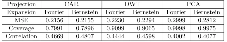
Expansion Fourier Bernstein Fourier Bernstein Fourier Bernstein MSE 0.2156 0.2155 0.2230 0.2294 0.2999 0.2812 Coverage 0.7991 0.7896 0.9099 0.9065 0.9998 0.9975 Correlation 0.4669 0.4807 0.4444 0.4598 0.4002 0.4077

First, we consider the cross-validation results for the models without using the dimension

reduction technique described in Section 1.4.1. Results are plotted in Figure 1.2 and appear in tables in Appendix C. Table 1.1 contains averages over all tilt angles, and Table 1.2 contains

averages over angles 20 through 70. In terms, the CAR projection with the Fourier expansion

predicts the log-CSP values most accurately. The coverages, however, indicate that the CAR model may not have adequate inferential properties, as only about 80% of the prediction

in-tervals contain the true value. The DWT projections are fairly accurate with moderately good

inferential properties, as indicated by the low MSE and coverages closer to the desired con-fidence. PCA projections yield inaccurate predictions that have low correlation with the true

values, but the prediction intervals have near perfect confidence.

Across all models, the predictive accuracy decreases when predicting at tilt angles 10 and

1_Φ_{= 100}_·_I

q,Ψ= 10·Iq,ν=p+ 2, anda=b= 0.1. For the DWT model, we setc=d= 0.1. For the CAR model, we setc=d= 0.1 and define adjacency as voxels that share a face, edge, or diagonal corner.

(26)

(a)Mean Squared Error

(b) Coverage (c) Correlation

Figure 1.2 Cross-validation results across all tilt tension angles.

(27)

80. This behavior is most likely be a result of these angles being on the outer edges of the domain. Prediction at these values would be extrapolation of the training data set, which is

generally less reliable than interpolation at the inner tilt angles.

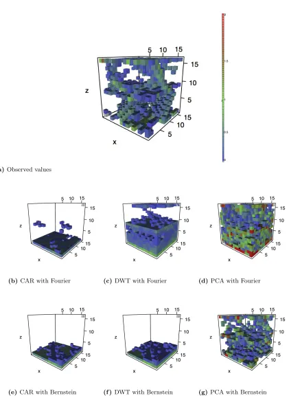
Next we visually inspect three-dimensional slice plots of cross-validation predictions. Figure 1.3 contains the observed and predicted values for tilt angle 10. The CAR and DWT models

do not capture the true values, predicting heavy defects throughout the lower half of the solid

but underestimating defects in the upper half. The twin-wall defect is not even apparent in the DWT projection with Bernstein polynomials. The PCA model overestimates defect intensity

but accurately locates defect structures.

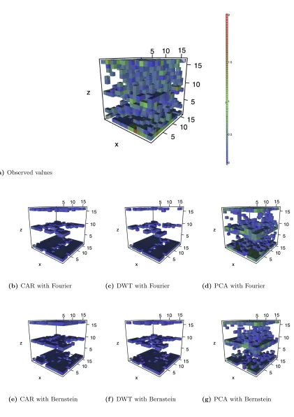
Figure 1.4 contains the observed and predicted values for tilt angle 50. The CAR model depicts some dislocations in the defect structures but smooths the intensity over the neighboring

voxels, particularly in the Bernstein expansion. DWT model appears biased towards predicting

the non-defective voxels that make up a large part of the solid, as only the twin-wall defect can be seen. PCA once again overestimates defect intensity, but dislocations and twin wall defects

are clearly represented.

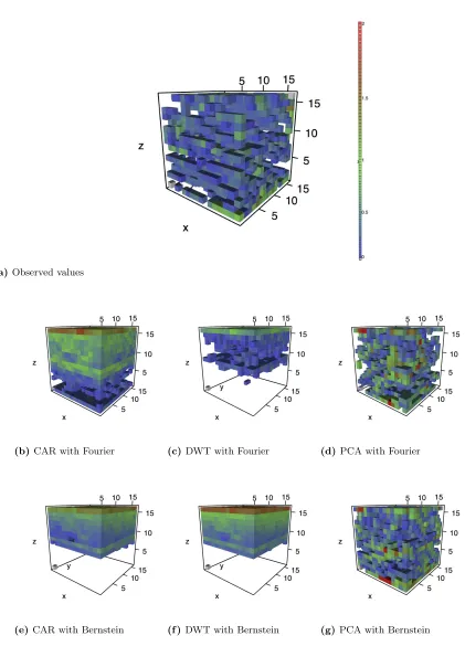
Figure 1.5 contains the observed and predicted values for tilt angle 80. Similar to the

behav-ior in tilt angle 10, the CAR and DWT models fail to accurately predict the dislocation defects,

though here they predict heavy defects in the upper half of the solid instead of the lower half. Similarly, the PCA model overestimates defect intensity but still locates the defect structures

throughout the solid.

Over all the tilt angles, the three-dimensional slice plots indicate that the PCA model is consistently better at predicting the location of the defect structures. The CAR and DWT

models assume that the data is spatially smoother than it actually is, leading to predictions

that fail to depict the dislocation defects.

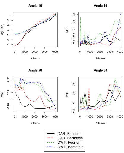
Finally, we consider how dimension reduction in the CAR and DWT models affects the

computation and prediction accuracy. Figure 1.6 plots computation time and the predictive

MSE against the number of terms retained in the model. Computation increases log-linearly in the number of terms, and the DWT models require generally more computation than the CAR

models. From the predictive MSE values, we see that the predictive accuracy either does not

improve or even decrease by having more model terms, particularly for the DWT models. More terms in the model leads to overfitting of the training data, which can exacerbate extrapolation

errors. Conversely, the predictive accuracy at the interpolation angles improves with more terms,

but the CAR model does not need as many terms as the DWT model to significantly improve the MSE.

(28)

(a)Observed values

(b) CAR with Fourier (c) DWT with Fourier (d) PCA with Fourier

(e)CAR with Bernstein (f )DWT with Bernstein (g) PCA with Bernstein

Figure 1.3 Predictions from cross-validation for tilt angle 10

Colored voxels distinguish defects due to high log-CSP values. Voxels with values below zero

(29)

(a)Observed values

(30)

(a)Observed values

(31)

Figure 1.6 Predictive accuracy dimension reduction results for CAR and DWT models

Horizontal axis indicates the number of rows of the projected data used in the training dataset, ranging from 10 to 163. Top-left figure shows the natural log of the computation time (in seconds) for angle 10 changing linearly with the number of terms; similar behavior is observed for other tilt angles.

(32)

1.6 Conclusion

We explored spatial functional models to predict the output images of molecular simulations.

Our objectives were to assess whether this is feasible and to evaluate the strengths and weakness of various approaches. For simulations involving interpolating predictions (angles 20 through

70), the mean squared error between predicted and observed was approximately 0.25, with

correlation 0.45. For simulations involving extrapolating predictions (angles 10 and 80) the mean squared error was significantly higher with lower correlation. Therefore, there is promise

that statistical prediction can be a useful supplement to numerical simulation for interpolation

purposes.

Of the spatial projection methods, PCA would be the preferred method for predicting plastic

damage. Despite being less accurate in terms of mean squared error, PCA captures the localized defects, which are by nature extreme values in the solid. CAR is consistently accurate even while

extrapolating, but the prediction intervals do not obtain their desired confidence. DWT leads to

fairly accurate prediction results with adequate inferential properties, but underestimates the defect structure in the lattice. For both CAR and DWT, dimension reduction vastly reduces

the computation time and may reduce errors in the prediction due to overfitting.

Further work could also explore the variation structures in the design conditions. This analysis focused solely on the final images of independent simulations using a single design

factor, but the model allows for more complex dependencies between the images. It would be

of particular interest to explore how the images change over the course of a single simulation, using the initial image to predict the probable final image.

In addition, analyzing the quantiles of the CSP distribution may be an interesting approach

to modeling material defects. Defective molecules have a high CSP but represent a small pro-portion of the total solid, so estimates and accuracy measures based on the mean may be

misleading. Therefore, a model for the upper quantiles of the CSP values in each voxel may

outperform a model for the average log-CSP. This extreme value analysis requires specialized techniques and distributions (such as the generalized Pareto distribution) but may improve

upon the predicted defect structures offered by the PCA spatial projections.

(33)

Chapter 2

Bayesian estimation of

crystallographic parameters through

weighted fusion of radiation

diffraction data

We develop a Bayesian model to accurately estimate crystallographic parameters from radiation diffraction data, an important concern in the field of crystallography and materials science.

Our model integrates measurements from multiple diffraction data sources using weighted data

fusion. Each diffraction data source is decomposed into the Bragg’s signal and background noise. The error has heterogeneous variance conditioned on the strength of the signal and a

variable weighting function that is estimated through Markov chain Monte Carlo (MCMC). This weighting function reduces the influence of less reliable or corrupted diffraction data,

leading to more accurate estimates of the crystallographic parameters. We perform a simulation

study that shows how variable weighting in the data fusion of X-ray and neutron diffraction significantly improves the crystallographic parameter estimates, particularly when we simulate

corruption in the data.

2.1 Introduction

In crystallography, diffraction is a powerful tool for identifying the atomic structure of materials.

Radiation waves, composed of either X-rays or neutron waves, are directed on a crystal lattice

(34)

and diffracted by the atoms. Bragg’s Law [BB13] predicts the diffraction angles given the value of various parameters about the lattice structure. Over the last century, efforts have been made

to observe and catalog the diffraction pattern for a variety of crystal and powder structures.

These efforts have led to massive databases of cataloged materials, such as the Materials Genome Initiative [Pab14].

The Rietveld Method [Rie69] minimizes the relative squared differences the observed and

theoretical scattering parameters. This method is the standard approach to estimating crystal-lographic parameters and has been implemented through software like the General Structure

Analysis System [LVD86; TVD13]. However, this method has been shown to be subject to errors

related to false minima and uncertainty quantification [Wil06]. More recently, work has been produced on applying Bayesian statistical modeling of atomic parameters from X-ray diffraction

data [BM11; GL16; Fan16].

Materials scientists are now commonly faced with the statistical challenge of coherently combining data from multiple sources, such as data of different measurement types or data

collected under different environmental conditions and different measurement devices. As a specific and important special case, we incorporate both X-ray and neutron diffraction data into

a Bayesian model to improve the estimation of the crystallographic parameters. Each radiation

source has its advantages and disadvantages [Est14], but combining the sources improves the estimates overall [Ush12; GL15; Zha15b].

For these data, we observe intensities over a range of scattering angles for two sets of

diffraction data,Y1(2θ) andY2(2θ), from two experiments on a crystal or powder material. The material of interest can be described bydcrystallographic parametersα= (α1, . . . , αd)T. These

diffraction signals are measured at n1 and n2 angles, respectively. The standard approach to estimating crystallographic parameters using data fusion minimizes

n1

X

i=1

W1(2θi)

[Y1(2θi)−Yˆ1(2θi;α)]2

Y1(2θi)

+

n2

X

i=1

W2(2θi)

[Y2(2θi)−Yˆ2(2θi;α)]2

Y2(2θi)

, (2.1)

where ˆY is the expected intensity for a material with crystallographic parametersα. In (2.1), Yk appears in the denominator to adjust for the larger variance for angles with higher intensity.

The weights Wk(2θi) determine the degree to which the measured intensity Yk at angle 2θi

affects the estimate forα. Naturally, ifWk(2θi) = 0, then the diffraction measure at that angle

is not used to estimate the crystallographic parameters. The weights are often taken to be constant for all angles,Wk(2θ) =wk. The user determines the weightsw1 and w2 based on the source that is deemed most reliable, and sensitivity to this choice is informally explored.

(35)

Here we present a method of estimating the weights for each source, yielding a data-driven fusion of the diffraction measures. The resulting estimated weight functions allow reliability

comparisons of the diffraction data intensities, both within each source and between the different

sources. In the following sections, we develop a Bayesian model that obtains both probabilistic estimates for the crystallographic parameters and weighting functions based on the uncertainty

of the data. This method is then used on simulation data to show how it improves the accuracy

of parameter estimates.

2.2 Statistical Model

We decompose thekth response into the signal Fk, the background scattering Bk, and random

errorEk

Yk(2θ) =Fk(2θ;α) +Bk(2θ) +Ek(2θ|α). (2.2)

The signal Fk depicts the true diffraction intensities as given by Bragg’s Law for given

crystal-lographic parametersα. The crystallographic parameters αare shared by all data sources, but

the data sources have separate background functions and independent errors.

The background scattering Bk(2θ) captures other signals in the mean that are not directly

related to the crystallographic parameters. The background is approximated as the linear

com-bination ofp spline functionsXj(·)

Bk(2θ) = p

X

j=1

Xj(2θ)βkj, (2.3)

with the prior assumption βkj iid

∼ Normal(0,1/φk) for the coefficients. Here we have assumed

the same basis expansion for all data sources, but this model can be easily generalized to have

a unique basis for each source.

After accounting for the signal and background scattering, the error process Ek(2θ) is

as-sumed to be independent overkand 2θ. As the intensities are count data, a Poisson distribution is a natural choice for the model [e.g. [BM11]], but the counts in crystallography are large enough to permit a normal approximation. Therefore, we assume the errors are Gaussian with mean

zero and variance proportional to the signalFk. The variance is

Var[Ek(2θ)|Fk(2θ;α)] =σ2k(2θi) =τ_k−1

h

1 +eδk_F

k(2θ;α)

i

eGk(2θ)_, _(2.4)

where τ_k−1 is the overall variance and eδk _{scales the signal’s effect on the variance. A one is}

(36)

added toeδk_F

k to avoid having zero variance at angles with no signal.

The function Gk(2θ) allows for heterogeneous variance across the diffraction angles. For

example, we might expect Gk(2θ) to be larger when there exists a discrepancy between the

signal and the data, and this model misspecification inflates the variance. To estimate the heterogeneous variance,Gk is expressed as the linear combination of q basis functions

Gk(2θ) = q

X

j=1 ˜

Xj(2θ)γkj (2.5)

as in (2.3). To ensure identification with the overall variance, we select basis functions with ˜

Xj(0) = 0 for alljand thuseGk(0) = 1, uniquely identifyingτk−1 as the variance for angles near

zero.

Under this model, twice the negative log-likelihood for a single source is

nk

X

i=1

logσk(2θi) +σ_k−2(2θi)[Yk(2θi)−Fk(2θi;α)−Bk(2θi)]2 .

For comparison with the data fusion equation in (2.1), this can be rewritten as

nk

X

i=1

logσk(2θi) +Wk(2θi)

[Yk(2θi)−Fk(2θi;α)−Bk(2θi)]2

[1 +δkFk(2θi;α)]

.

where

Wk(2θ) =e−Gk(2θ) (2.6)

measures the precision of data source k at angle 2θ. As a result, twice the joint negative log-likelihood of the X-ray and neutron data

n1

X

i=1

logσ1(2θi) +W1(2θi)

[Y1(2θi)−F1(2θi;α)−B1(2θi)]2

[1 +δ1F1(2θi;α)]

+ n2 X i=1

logσ2(2θi) +W2(2θi)

[Y2(2θi)−F2(2θi;α)−B2(2θi)]2

[1 +δ2F2(2θi;α)]

(2.7)

which resembles (2.1) with Wk(2θ) as the weight function. This weighting function effectively

decreases the influence of angles with high error variance, whether it results from natural

variability in the intensity counts or through model misspecification.

(37)

2.3 Computational Details for Parameter Estimation

In order to perform Markov chain Monte Carlo (MCMC) and obtain estimates of the

crystallo-graphic parameters, we must first derive the posterior distributions for the model parameters. First, we express the model in Equation (2.2) in the following vector form

Yk=Fk+Bk+Ek (2.8)

where

Yk = [Yk(2θ1), . . . , Yk(2θnk)]

T_;_F

k= [Fk(2θ1;α), . . . , Fk(2θnk;α)]

T_,

Bk = [Bk(2θ1), . . . , Bk(2θnk)]

T_;_E

k = [Ek(2θ1), . . . , Ek(2θnk)]

T_.

Equation (2.3) is expressed asBk=Xβk, wherexi = [X1(2θi), . . . , Xp(2θi)]T,X= (xT1, . . . ,xTn)T,

and β_k= (βk1, . . . , βkp)T.

2.3.1 Background and Precision Parameters The full conditional distribution forβ_k is

β_k|rest∼Normal

(

V

n

X

i=1

Wk(2θi)[Yk(2θi)−Fk(2θi;α)]xi,V

) (2.9) where V= " _n X i=1

Wk(2θi)xixTi +φkIp

#−1

. (2.10)

For the precision parameters, we assume the prior distribution τk, φk∼Gamma(a, b), yielding

the following full conditional distributions:

τk|rest ∼ Gamma

"

a+nk 2 , b+

1 2

X

i

[Yk(2θi)−Fk(2θi)−xTi βk]2e−Gk(2θi)

1 +eδkF_k(2θ_i)

#

(2.11)

φk|rest ∼ Gamma

"

a+p 2, b+

P

jβkj2

2

#

. (2.12)

We obtain posterior samples ofδk andγkj using a random-walk Metropolis-Hastings algorithm

with Gaussian candidate distributions and regular tuning for an the acceptance rate between 20% and 50%.

(38)

2.3.2 Crystallographic Parameters

For the crystallographic parameters, we denote the range of physically plausible values for αl

as [Ll, Ul]. In the examples considered here, we have two cases: bounded parameters with finite |Ll| and |Ul|, and one-sided bounds with |Ll| < ∞ and Ul = ∞. In the first case, we select

a Uniform prior, αl ∼ Uniform(Ll, Ul), and in the second case, we select a log-Normal prior,

log(αl−Ll)∼Normal(0,1). For MCMC sampling, we transform the crystallographic parameters

αl into normally distributed latent variablesZl using the transformations

Zl=

    

Φ−1

αl−Ll

Ul−Ll

, Ul <∞

log(αl−Ll), Ul =∞

. (2.13)

where Φ−1is the inverse cumulative density function of the normal distribution. After obtaining

posterior estimates for the latent variables, we transform Zl back into the original

crystallo-graphic parameter

αl=

(

Ll+ (Ul−Ll)Φ(Zl), Ul<∞

Ll+ exp(Zl), Ul=∞

(2.14)

where Φ is the cumulative density function of the normal distribution. We use a random-walk Metropolis-Hastings algorithm to obtain posterior samples ofZl with Gaussian candidate

distributions and regular tuning for an the acceptance rate between 20% and 50%.

2.4 Simulation Study

The simulation study explores two questions of interest regarding crystallography. First, we

explore whether the fusion of both X-ray and neutron diffraction data significantly improves estimation of crystallographic parameters compared to using only one data source. Second, we

assess the ability of the proposed data fusion approach to identify reliable information and its

performance gain over more naive fusion approaches.

2.4.1 Data Generation

To generate the data, we set the crystallographic parameters to fixed values and generate a

synthetic signal for both the X-ray and neutron data. The synthetic signal Fk is calculated

from

Fk(2θ) =I0

X

hkl

SFhklL(2θ)H(λ,2θ0, U, V, W) (2.15)

(39)

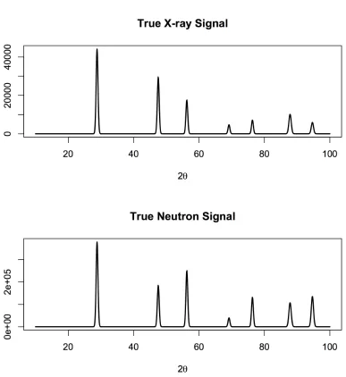
Figure 2.1 True X-rayF1(2θ) and neutronF2(2θ) signals

Signals used in the simulation study, plotted by scattering angle 2θ.

(40)

where L(2θ) represents the Lorentz-polarization correction and SFhkl represents the structure

factors of gold [Fan16]. The vector α contains six parameters: incident intensity (I0),

wave-length (λ), angle offset (2θ0), and Caglioti parameters (U,V, andW). For this study, data was generated using I0 = 101, λ= 1.53, 2θ0 = 0.57, U = 7·10−7, U =−3·10−5, and W = 0.04. The resulting curves are plotted in Figure 2.1.

For the simulated X-ray data, we use the following functions for the true background function

B1 and heterogeneous variance function G1

B1(2θ) = 5 4cos 2θ 4 +2θ 25sin 2θ 3 , G1(2θ) =

2θ 30cos 2θ 4 +2θ 40sin 2θ 3 .

For the simulated X-ray data, we use the following functions for the true background function B2 and heterogeneous variance function G2

B2(2θ) = 100 2θ cos 2θ 4

+ 2 sin

2θ 3

, G2(2θ) =

10 2θcos 2θ 4 +60 2θsin 2θ 3 .

We construct the error variance using Equation (2.4), withτ = 5 andδ = log(0.001).

To study the model’s ability to identify reliable information, we simulate corruption in the data using an incorrect mean with signal set to zero for some angles. For X-ray signals, angles

in the upper third of the domain were corrupted

F₁C(2θ;α) =

(

F1(2θ;α), 2θ <66.7

0, otherwise. (2.16)

For neutron signals, angles in the lower third of the domain were corrupted

F₁C(2θ;α) =

(

F1(2θ;α), 2θ >33.3

0, otherwise. (2.17)

We simulate data with corruption in both, one, or neither data source. For each of these

sce-narios, we generate 100 data sets. Each simulated data set is fit using either X-ray data only,

neutron data only, or both data sources. We also fit the data either allowing the weighting function to vary across angle or be constant (i.e. Gk(2θ) = 0 for all θ). For all models, we

(41)

use p= 20 spline basis functions for the background. For models with varying weight, we use q = 10 spline basis functions to fit Gk, with the restriction that Gk(0) = 0. For each fit of the

simulated data, we generate 2000 MCMC samples and discard the first 1500 as burn-in.

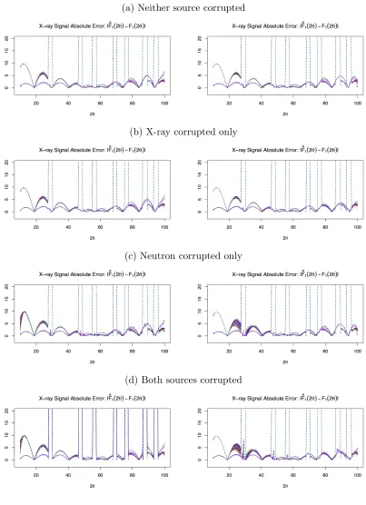
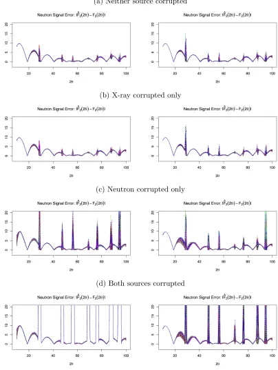
2.4.2 Results and Discussion

Figures 2.2 and 2.3 contain plots of the posterior means for the signal absolute error|Fˆk(2θ)−

Fk(2θ)|. Figures 2.4 and 2.5 contain plots of the posterior means for the background scattering

ˆ

Bk(2θ). Figure 2.6 contains plots of the posterior means for the log of the weighting functions

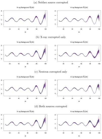
logWk(2θ) =−Gˆk(2θ). For these plots, we considered either both sources corrupted or neither

source corrupted. Each data set was fit using both sources, with either constant or varying

weights. These figures illustrate how the weighting function reacts to data corruption and affects the estimated background scattering and signal. When the data are corrupted, the signal’s effect

on the parameter estimate is decreased overall, as shown by the scales in the weighting functions.

TheGkfunction compensates for the decreased signal effect, but the varying weight has greater

freedom to adjust. The varying weight decreases around the corrupted angles, but the constant

weight decreases over all of them. The estimated background scattering has higher variability at

angles with lower weight, so the varying weight function leads to better fits of the background for both corrupted and uncorrupted data sources. As a result, the varying weight leads to less

absolute error in the signal, particularly at the peaks.

Tables 2.1 and 2.2 contain means and standard errors for squared relative errors for the crystallographic parameters estimates. The squared relative error is calculated as

( ˆαl−αl)2

α2

l

(2.18)

where ˆαl is the posterior mean and αl is the true value used in the data generation. Tables

2.3 and 2.4 contains coverage proportions of 95% credible intervals for the crystallographic

parameters.

Overall, the data fusion model with varying weights offers consistently accurate parameter

estimates. The MSE and coverages for the fusion model with varying weights are competitive

with the best models across all scenarios. When the neutron data are not corrupted, the model with only neutron data and constant weight has the smallest MSE values, but if it is corrupted,

the MSE and coverages for the parameters for this model are significantly worse than the other models, particularly for the initial intensity I0 and Cagliotti parametersU,V, and W. For the X-ray models, the varying weights always lead to improved accuracy in the MSE.

(42)

(a) Neither source corrupted

(b) X-ray corrupted only

(c) Neutron corrupted only

(d) Both sources corrupted

Figure 2.2 Absolute error between fitted and true X-ray signal for simulated data sets.

Lines represent fitted function from each simulation based on the posterior means. Left side plots used constant weighting; right side plots used variable weighting.

(43)

Figure 2.3 Absolute error between fitted and true neutron signal for simulated data sets.

(44)

Figure 2.4 Fitted X-ray background scattering for simulated data sets.

(45)

Figure 2.5 Fitted neutron background scattering for simulated data sets.

(46)

Figure 2.6 Fitted variable weighting functions for simulated data sets.

Lines represent fitted function from each simulation based on the posterior means. Left side plots are for X-ray diffraction; right side plots are for neutron diffraction.