Division V
LARGE-SCALE PARALLEL COMPUTING PERFORMANCE OF
FINITE ELEMENT ANALYSES FOR REACTOR BUILDING
INCORPORATING SOIL-STRUCTURE INTERACTION
Yoshiyuki Takahashi1, Naoki Morita2, Toshihide Saka3,Gaku Hashimoto4, Hiroshi Okuda5 and Kazuhiko Yamada6
1 Structural Engineer, Nuclear Power Department, Kajima Corporation, JAPAN
2 Graduate Student, Graduate School of Frontier Sciences, The University of Tokyo, JAPAN 3 Senior Research Engineer, Technical Research Institute, Kajima Corporation, JAPAN 4 Lecturer, Graduate School of Frontier Sciences, The University of Tokyo, JAPAN 5 Professor, Graduate School of Frontier Sciences, The University of Tokyo, JAPAN 6 Senior Manager, Nuclear Power Department, Kajima Corporation, JAPAN
ABSTRACT
This paper presents the large-scale parallel computing performance of finite element (FE) analysis for a reactor building incorporating soil-structure interaction by using the open-source FE program, FrontISTR. A FE model whose scale is similar to that employed in existing practices is used to confirm the accuracy as the original model. A large-scale model is created by refining the original model as the refined model to investigate the parallel efficiency of the FE solver. The concept of the domain decomposition method is incorporated to perform highly efficient parallel computation of the conjugate gradient solver with block diagonal scaling.
Numerical analyses are executed with different numbers of processors that correspond to those of the decomposed domains. Based on the analysis results, the efficiency of parallelization to soil-structure interaction problems is examined. For evaluating the scalability of the program and data, the normalized speed-up factor (NSF) is defined. Using the NSF, a reasonable number of parallel processes is proposed. If the parallelization ratio and NSF are given, a reasonable number of parallel processes can be obtained. In case that the NSF is 50%, reasonable numbers of processes are respectively estimated as 322 for the original model and 2247 for the refined model.
INTRODUCTION
The sway-rocking model or the lattice model, which is classified as a lumped mass model, is widely used for seismic response analysis of nuclear facilities in which various responses, such as acceleration response, shear strain, and the ground contact ratio, are calculated. If the ground contact ratio becomes less than 50%, a response analysis is performed by utilizing a mixed model of the lumped mass model as a structure and the finite element (FE) model as soil with consideration for the contact behavior between the base mat of the structure and the soil.
In this paper, as the first step in a series of studies, a linear dynamic response analysis is conducted with soil-structure interaction using two FE models of different sizes in terms of the numbers of degrees of freedom. Whereas the scale of one of the FE models is similar to that employed in existing practices, the other model scale is larger. A domain decomposition method and a parallel iterative solver are utilized to execute large-scale FE analysis. For evaluating the scalability of program itself and performing effective parallel computing, the normalized speed-up factor is defined and a reasonable number of parallel processes is proposed.
FINITE ELEMENT MODELS
Original Model
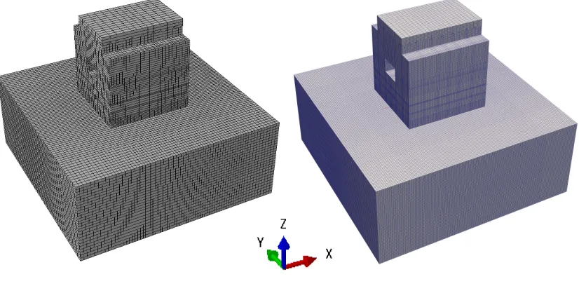
Figure 1 (a) shows the FE model of a reactor building with surrounding soil. The building part sizes are approximately 60 m square and 65 m in height, and the soil part sizes are 150 m square and 60.8 m in depth. The soil and base mat are modeled by solid elements, whereas the other parts are modeled by shell elements in order to reduce the number of degrees of freedom of the whole model and the number of computational tasks. The soil surface mesh is not consistent with that of the base mat, so these meshes are combined by multipoint constraints (MPC). The MPC coefficients are determined using the shape functions of FEs. The columns, beams, and roof trusses of the building are omitted for model simplification, so equivalent properties are given for shell elements corresponding to them.
(a) Original. (b) Refined.
Figure 1. FE models combined soil and structure.
Mesh Refinement
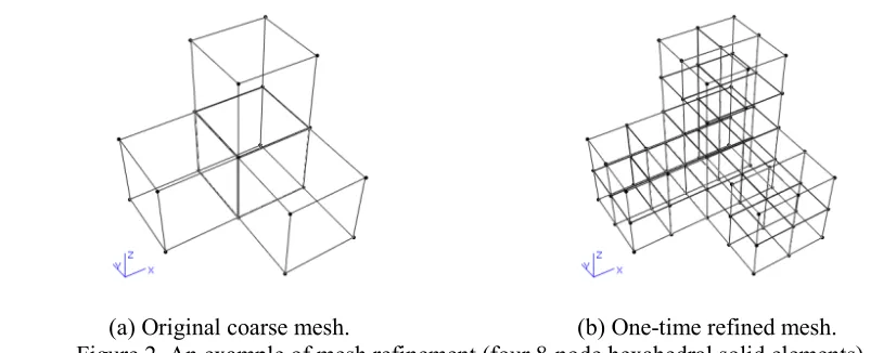
(a) Original coarse mesh. (b) One-time refined mesh. Figure 2. An example of mesh refinement (four 8-node hexahedral solid elements).
Model Specifications
Based on the above technique, a refined FE model is made from the original model as shown in Figure 1 (b). As analysis models, both the original model and the refined model are adopted. Table 1 shows the specifications of the two FE models. The total number of degrees of freedom of the refined model is about seven times as large as that of the original model. Table 2 shows the material properties of the building and soil. It is assumed that the design strength of concrete for the building is 33 N/mm2 and
the shear wave velocity of the soil is uniformly about 700 m/s. Stiffness-proportional damping whose reference frequency is 3.4 Hz is set for the transient analysis.
Table 1. Specifications of FE models.
Part Original model Refined model
Node number Building Soil 30,411 145,124 147,017 1,124,475
Total 175,535 1,271,492
Element number Building Soil 18,840 136,080 99,840 1,088,640
Total 154,920 1,188,480
Number of Degrees of freedom
Building 91,233 441,051
Soil 435,372 3,373,425
Total 526,605 3,814,476
Table 2. Material properties.
Building (Concrete) Soil
Design strength [N/mm2] 33 -
Shear wave velocity [m/s] - 700
Density [t/m3] 2.4 2.0
Young’s modulus [kN/m2] 2.52×10⁷ 2.6×10⁶
Poisson ratio [-] 0.2 0.3
PARALLEL FINITE ELEMENT PROGRAM: FrontISTR
Outlines
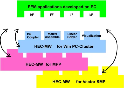
In this study, FrontISTR, which is an open-source parallel FE program for nonlinear structural analysis, is used for the parallel FE analysis. Various nonlinear analysis functions of FrontISTR are implemented utilizing the middleware called HEC-MW (High End Computing-Middleware), which supports common operations in the FE method and hides hardware dependency, particularly the dependency on parallel architectures, from the application developers. Since the efficiency, portability, and maintainability of the FE programs are assured by HEC-MW, it enables customization of FrontISTR while keeping the ability of efficient large-scale parallel analysis, for example, to add user-developed elements.
High End Computing-Middleware: HEC-MW
HEC-MW provides the Application Programming Interfaces (APIs), which are commonly usable in developing various purpose FE applications. Thus, HEC-MW is classified as the upper-level libraries for developing the various kinds of FE applications. The APIs are mainly for (1) large-scale parallel FE data and its input/output (I/O), (2) matrix profile information, (3) matrix assembling, (4) parallel linear equation solvers, (5) parallel visualization, (6) interface for coupled analysis, and (7) utilities for domain decomposition. Figure 3 shows the plug-in image of developing FE applications running on various computer architectures.
Figure 3. Development of FE applications with HEC-MWs for various computer architectures.
HEC-MW adopts the Single-Program Multiple-Data (SPMD) programing model as shown in Figure 4. A whole domain discretized by FE mesh is decomposed into distributed local subdomains. A communication table, which represents the connection information among subdomains, is generated at the domain decomposition. Each subdomain is assigned to a computer node (CPU, core, etc.), and local FE operations, for example, the element matrix constructions, are done in parallel, while global operations using the Message Passing Interface (MPI) occur only in the linear equation solvers. Since MPI communications, OpenMP operations, hardware-dependent operations, re-ordering, I/O for parallel FE analysis, etc., are hidden behind the APIs of HEC-MW, a FE parallel program built on HEC-MW can be seen as if it were a serial program.
HEC MW- for Vector SMP
for MPP HEC-MW
Visualization Linear
Solver AssembleMatrix
Coupler I/O
Cluster -for Win PC MW
-HEC
FEM applications developed on PC
I/F I/F
Figure 4. SPMD programming style of FrontISTR (HEC-MW).
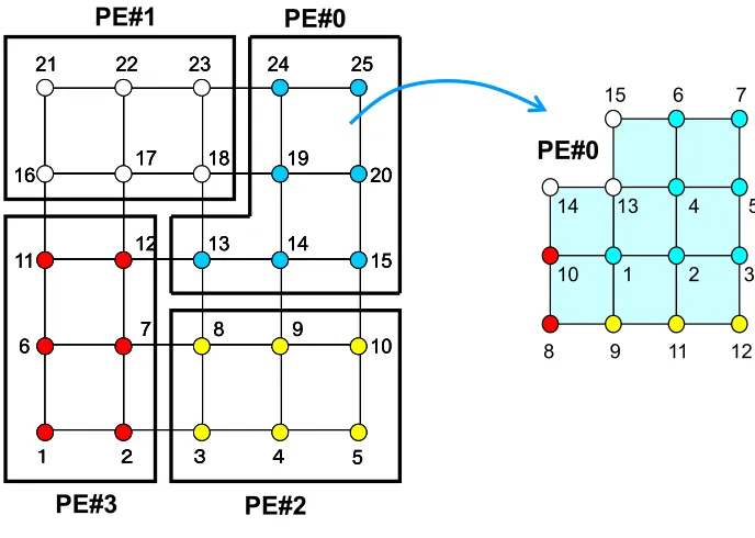
The local data structure of HEC-MW is based on the node-based decomposition as shown in Figure 5. Each subdomain holds the data of the matrices and vectors not only for the subdomain’s own but also for the overlapped regions, which is typically a one-element depth layer. The depth of the overlap works for the effect of preconditioners used in iterative solvers. Domain decomposition and generation of communication tables are done by Metis, which is one of the most used of the graph partitioning software programs.
Figure 5. Local data structure of HEC-MW.
Iterative Solver
From the point of view of the parallel programing model, a message passing by MPI for inter-node parallelization and loop directives by OpenMP for intra-inter-node parallelization, that is, a hybrid model, appear to be appropriate. Vectorization (reordering) is also considered to take advantage of more inner parallelization.
Local Data
Local Data
Local Data
Local Data
MPI
MPI
MPI Solver Subsystem
Solver Subsystem
Solver Subsystem
Solver Subsystem FEM Code
FEM Code
FEM Code
FEM Code
1 2 3
4 5
6 7
8 9 11
10 14 13
15
12 PE#0
1 2 3 4 5
21 22 23 24 25
16 17 18 19 20
11 12 13 14 15
6 7 8 9 10
1 2 3 4 5
21 22 23 24 25
16 17 18 19 20
11 12 13 14 15
6 7 8 9 10
PE#0 PE#1
PE#2 PE#3
1 2 3 4 5
21 22 23 24 25
16 17 18 19 20
11 12 13 14 15
Such a programing model has a significant relationship to the data structure of the parallel FE model. As described in Figure 5, in HEC-MW, which FrontISTR is built on, the entire domain (= FE mesh) is partitioned into distributed local data sets, and each subdomain is assigned to a node with (1) local operation and no global dependency for a subdomain computation, (2) continuous memory access, and sufficiently long loops by reordering. Since the iterative equation solver is one of the most important kernels in FrontISTR, how the domain decomposition works in the preconditioned iterative solver is described below.
Operations of most preconditioned iterative solvers are a combination of the following: (i) Matrix–vector products
(ii) Inner dot products
(iii) DAXPY (a x + y) and vector scaling (iv) Preconditioning operations
DYNAMIC RESPONSE ANALYSIS
Analysis Conditions
Linear transient analysis is conducted to verify the practicality of FrontISTR to soil-structure interaction problems using the original model and the refined models. The bottom of the soil is fixed as the boundary conditions. An earthquake load is applied as the inertial force in the X-direction. The input motion is the NS component of El Centro wave observed on the Imperial Valley earthquake in 1940. The time increment and duration time are set to 0.001 s and 4.0 s respectively, and the Newmark-β method (β = 0.25) is selected as the time integration method. The conjugate gradient (CG) method is utilized as the solver of a system of linear equations, and the convergence tolerance for the CG solver is set to 1.0 × 10⁻⁸. The block diagonal scaling is employed as the preconditioning for the CG solver, and the number of
processors is set to 128 as the flat MPI parallelization. The supercomputer Oakleaf FX-10 owned by The University of Tokyo is used for the whole analysis.
Analysis Results
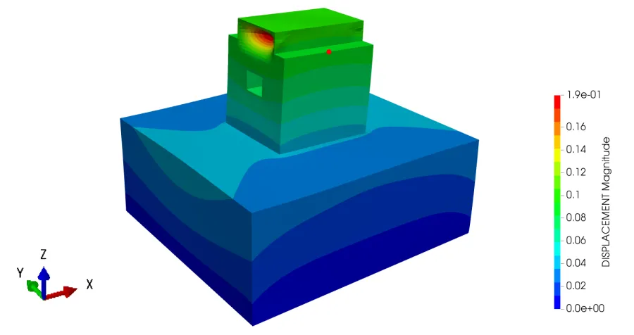
Figure 6. Deformation snapshot with relative displacement contour. (Red point is the representative node for Figure 7.)
Figure 7. Relative displacement responses of representative nodes on the building.
Table 3. Maximum response values of representative nodes on the building.
(*) means the relative error with respect to the response of the original model for FrontISTR. Relative responses Original model Abaqus Original model FrontISTR Refined model
Acceleration [m/s2] -23.36
(0.09%) -23.38 (-) (1.28%) -23.68 Velocity [m/s] (0.07%) 1.408 1.409 (-) (1.21%) 1.426
Displacement [m] (0.11%) .09315 .09325 (-) (1.50%) .09465 -0.1
-0.05 0 0.05 0.1
0 0.5 1 1.5 2 2.5 3 3.5 4
R
el
at
iv
e d
is
pl
acem
en
t [
m
]
time [s] Original : Abaqus
PARALLELIZATION PERFORMANCE
Evaluation of Parallelization Performance
Based on the above analysis data, the efficiency of parallelization is examined. As is well known, the speed-up factor Sp and the parallel efficiency Ep are expressed below.
p s
p T
T
S = (1)
p S
E p
p = (2)
where Ts is the calculation time of serial processing, Tp is the calculation time of parallel processing, and
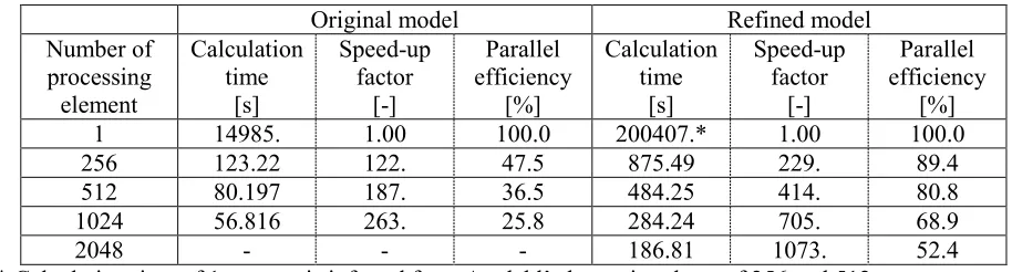
p is the number of parallel processes. Table 4 shows examples of the parallelization performance of the linear dynamic response analyses measured for the first 100 steps. The parallelization performance differs between the original model and the refined model. The numbers of processes such that the parallel efficiency is approximately 50% are 256 for the original model and 2048 for the refined model. Also, the parallelization ratios inferred from the analysis results are 99.69046% and 99.95552% for each model.
Table 4. Examples of parallelization performance.
Original model Refined model
Number of processing element Calculation time [s] Speed-up factor [-] Parallel efficiency [%] Calculation time [s] Speed-up factor [-] Parallel efficiency [%]
1 14985. 1.00 100.0 200407.* 1.00 100.0
256 123.22 122. 47.5 875.49 229. 89.4
512 80.197 187. 36.5 484.25 414. 80.8
1024 56.816 263. 25.8 284.24 705. 68.9
2048 - - - 186.81 1073. 52.4
* Calculation time of 1 process is inferred from Amdahl’s law using those of 256 and 512 processes.
Evaluation of Reasonable Number of Parallel Processes
The speed-up factor Sp is also expressed using the parallelization ratio α, whereas the
parallelization ratio is a ratio of parallelizable time to the whole calculation time on serial processing. Also, the maximum speed-up factor Sp max is obtained, and the normalized speed-up factor (NSF) SpN is
defined as follows.
p
Sp α
where pN α p α −
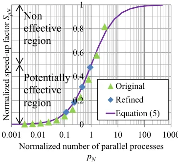
=1 is the normalized number of parallel processes, and the SpN range is 0≤SpN ≤1. Figure 8 (a) shows the relationships between the number of parallel processes and the speed-up factor. Approximate curves are illustrated by substituting the parallelization ratios obtained in the previous section into Equation (3). The speed-up factor is a function of the parallelization ratio and the number of parallel processes; consequently, it is difficult to evaluate the scalability of the combination of the program and data. Consistent discussions become possible by the normalizing speed-up factor. Figure 8 (b) describes the relationships between the normalized number of parallel processes and the normalized speed-up factor. Equation (5) is adaptable to any parallelization ratio. The NSF of the original model is greater than 50%, which means further parallelization is not effective. On the other hand, the NSF of the refined model is approximately 50%, which means that parallelization is effective.
The concept of the reasonable number of parallel processes is introduced for effective parallel computing. The reasonable number of parallel processes pR is defined below. If the parallelization ratio
and the NSF are given, the reasonable number of parallel processes can be obtained.
) 1 )( 1 ( pN pN R S S p − − = α α (6)
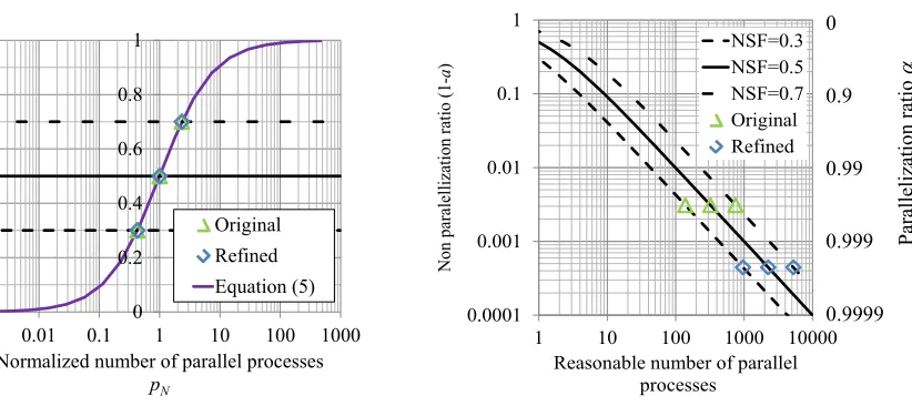
Table 5 and Figure 9 illustrate evaluation examples of the reasonable number of parallel processes. Here, NSFs are set to 0.3, 0.5, and 0.7 as examples. As a result, the reasonable numbers of parallel processes where the NSF is 50% are, respectively, 322 for the original model and 2247 for the refined model.
(a) Ordinary relationships. (b) Normalized relationships. Figure 8. Relationships between number of parallel processes and speed-up factor.
Table 5. Examples of reasonable number of parallel processes.
Original model Refined model Variables
Parallelization ratio 99.69046% 99.95552% α
Normalized speed-up factor 70% 50% 50% 30% SpN
Reasonable number of
parallel processes 751 322 2247 963 pR
1 10 100 1000 10000
1 10 100 1000 10000
Sp eed -u p fact or Sp
Number of parallel processes p
Original Refined Equation (3) 0 0.2 0.4 0.6 0.8 1
0.001 0.01 0.1 1 10 100 1000
N or m al ized sp eed -up fa ct or SpN
Normalized number of parallel processes
(a) Setting of normalized speed-up factor. (b) Conversion to number of parallel processes. Figure 9. Evaluation procedures of reasonable number of parallel processes.
CONCLUSION
In this paper, as the first step in a series of studies, a linear transient analysis is performed with soil-structure interaction using a finite element model of a reactor building with the surrounding soil (original model) and its refined model. The domain decomposition method and conjugate gradient solver with block diagonal scaling are utilized throughout the study. Based on the analysis results, the efficiency of parallelization in soil-structure interaction problems is examined.
In a comparison between the analysis results of FrontISTR, an open-source finite element program, and Abaqus using the original model, it is confirmed that FrontISTR has sufficient calculation accuracy. The numbers of processes where parallel efficiency is approximately 50% are, respectively, 256 for the original model and 2048 for the refined model, and the parallelization ratios are 99.69046% and 99.95552% for each model.
For evaluating the scalability of a combination of the program and data and for effective parallel computing, the normalized speed-up factor is defined and the concept of a reasonable number of parallel processes is proposed. If the parallelization ratio and normalized speed-up factor are given, a reasonable number of parallel processes can be obtained. If the normalized speed-up factor is 50%, the reasonable numbers of processes are, respectively, 322 for the original model and 2247 for the refined model.
REFERENCES
Nakajima K. and Okuda, H. (2004). “Parallel iterative solvers with selective blocking preconditioning for simulations of fault-zone contact,” Numerical Linear Algebra with Applications, Vol. 11, Issue 8-9, pp. 831-852.
Okuda, H. and Yagawa, G. (2005). “Large-Scale Parallel Finite Element Analysis for Solid Earth Problems by GeoFEM,” Surveys on Mathematics for Industry, pp.159-196.
Takahashi, Y., Saka, T., Koiso, T. and Yamada, K. (2015). “Finite element method for soil-structure model consisting of four million degrees of freedom,” Summaries of Technical Papers of Annual Meeting, Architectural Institute of Japan, JP, Structures II, pp.303-306. (In Japanese)
http://www.ciss.iis.u-tokyo.ac.jp/rss21/theme/multi/heckernel/index.html (In Japanese) http://www.ciss.iis.u-tokyo.ac.jp/riss/project/structure/ (In Japanese)
http://glaros.dtc.umn.edu/gkhome/views/metis 0 0.2 0.4 0.6 0.8 1
0.001 0.01 0.1 1 10 100 1000
N or m al ized sp eed -up fa ct or SpN
Normalized number of parallel processes
pN Original Refined Equation (5) 0.0001 0.001 0.01 0.1 1
1 10 100 1000 10000
N on pa ra le lli za tion ra tio (1 -a )