Force Feedback Control of Tool Deflection in Miniature Ball End Milling.

(1)

ABSTRACT

HOOD, DAVID WAYNE. Force Feedback Control of Tool Deflection in Miniature Ball End Milling. (Under the direction of Dr. Gregory Dale Buckner.)

(2)

(3)

FORCE FEEDBACK CONTROL OF TOOL

DEFLECTION IN

MINIATURE BALL END MILLING

by

DAVID WAYNE HOOD

A thesis submitted to the Graduate Faculty of North Carolina State University

in partial fulfillment of the requirements for the Degree of

Master of Science

MECHANICAL ENGINEERING

Raleigh 2003

APPROVED BY:

________________________________ _______________________________

(4)

ii This work is dedicated to the glory and honor of

my personal Lord and Savior, Jesus Christ.

(5)

iii

BIOGRAPHY

(6)

iv

ACKNOWLEDGMENTS

There are many people I would like to thank who have been instrumental in my completion of this degree. The patience and support of all of those around me have been a tremendous help and is greatly appreciated. I would first like to thank Dr. Gregory D. Buckner, my advisor, for taking me as a student and being an excellent mentor: thanks also for being a good friend. I would like to thank Dr. Thomas A. Dow for his support and insight at the Precision Engineering Center. His help in developing the necessary skills to conquer real world problems and thoroughness is the foundation of the Precision Engineering Center and is greatly appreciated. Thank you to Alex for help with machining and for offering support in the weekly discussions about which is better – model or stiffness based closed-loop control. Thanks to Ken for all the PMAC help as well as Maple and MATLAB programming – he never minded taking time to help with the project. Thank you to Dr. Ron O. Scattergood for being on my committee and for his insight. Thank you as well to Laura for all her administrative help and purchase orders. Also to all the students at the PEC I want to thank you for the great times we had, the great discussions, and friendships developed over the past year. I especially want to thank Stuart Clayton, David Gill, David Kametz, Patrick Morrissey, Nobu Negishi, Witoon Panusittikorn, and Travis Randall.

I want to thank my mom, dad, and brother who have always been there for me with love and support, telling me I can do anything, and that I should never compare myself to anyone else, but to just be the best I can be. Thank you especially to my dad for allowing me to work with him the past 10 years – his attitude of perfection, work ethic, and hand skills I’ve both inherited and learned from watching him, and he has given me an education not available in school. You have no idea how much you all mean to me and I will always remember your words of wisdom.

(7)

v you mean to me and I want you to know I love you. You’re an inspiration and I sincerely appreciate all your prayers, support, and for always being there for me.

(8)

vi

LIST OF TABLES

Table 1 Measured and computed stiffness values for long shank, ball end

tools……… 9

Table 2 Ziegler-Nichols ultimate stability tuning criteria [13] and gains for

axes.……… 19

Table 3 System

frequencies………...……….….……… 23

Table 4 Cross-correlation coefficients for uncompensated linear slotting

cut………... 63

Table 5 Cross-correlation coefficients for compensated linear slotting cut

……….………... 65

Table 6 Cross-correlation coefficients for compensated linear slotting cut with

new maximum force capture...………... 73 Table 7 Large groove experimental results: deflection compensation vs.

(11)

ix

LIST OF FIGURES

Figure 1: Long shank, ball end milling tool: geometry and force components... 5

Figure 2: Depth vs. force curve derived from the non-dynamic cutting force model ... 6

Figure 3: Nanoform DTM machine and setup... 7

Figure 4: Workpiece mounted on three-axis piezoelectric load cell ... 8

Figure 5: Measured and predicted orthogonal cutting forces: 25 degree tool tilt... 8

Figure 6: Experimental force vs. deflection curve at 25 degree tilt (added linear trendline) ... 11

Figure 7: Tool deflection with desired and actual depth ... 12

Figure 8: Diagram of predicted depth algorithm ... 13

Figure 9: Diagram of predicted deflection algorithm ... 15

Figure 10: Ziegler-Nichols ultimate stability tuning criteria [13] ... 19

Figure 11: PID axis controllers: tuned step responses, 0.1 mm... 20

Figure 12: z-force at 25 degree tilt cutting ... 24

Figure 13: Diagram of dSPACE peak and hold algorithm ... 26

Figure 14: Bode plot of Butterworth 5th order filter characteristics ... 27

Figure 15: dSPACE cutting force and maximum force capture ... 28

Figure 16: z-plane for a discrete system ... 30

Figure 17: Unit step input responses of a first-order digital filter with differing coefficients ... 32

Figure 18: Time constant of first-order digital filter ... 33

Figure 19: Small groove experimental setup ... 35

Figure 20: Small groove Talysurf alignment procedure... 37

Figure 21: PMAC acquired cutting force vs. actual cutting force ... 38

Figure 22: PMAC acquired cutting force and filtered force... 39

Figure 23: Predicted deflection during uncompensated cut without multiplication factor . 40 Figure 24: Experimental profile measurements: predicted depth compensation, linear slotting cut ... 41

Figure 25: Experimental profile errors: predicted depth compensation, linear slotting cut 42 Figure 26: Experimental profile measurements: predicted deflection compensation, linear slotting cut ... 44

Figure 27: Experimental force measurements: predicted deflection compensation, linear slotting cut ... 45

Figure 28: Experimental profile errors: predicted deflection compensation, linear slotting cut ... 46

Figure 29: Experimental profile measurements: predicted deflection compensation, one period sinusoidal slotting cut ... 47

(12)

x Figure 31: Experimental profile errors: predicted deflection compensation, one period

sinusoidal slotting cut ... 49

Figure 32: Experimental profile measurements: predicted deflection compensation, two period sinusoidal slotting cut ... 50

Figure 33: Experimental force measurements: predicted deflection compensation, two period sinusoidal slotting cut ... 51

Figure 34: Experimental profile errors: predicted deflection compensation, two period sinusoidal slotting cut ... 52

Figure 35: Experimental profile repeatability errors: predicted deflection compensation, linear slotting cut ... 54

Figure 36: Experimental profile repeatability errors: predicted deflection compensation, one period sinusoidal slotting cut ... 56

Figure 37: Experimental profile repeatability errors: predicted deflection compensation, two period sinusoidal slotting cut ... 57

Figure 38: Experimental force measurements: filtered and captured maximum cutting force, uncompensated linear slotting cut ... 60

Figure 39: Experimental profile measurement: uncompensated linear slotting cut ... 61

Figure 40: Experimental workpiece surface profile measurement before cutting... 62

Figure 41: Experimental force measurements: Butterworth and maximum force capture, compensated linear slotting cut ... 64

Figure 42: Experimental profile measurement: compensated linear slotting cut ... 65

Figure 43: Old maximum force capture algorithm ... 67

Figure 44: Improved maximum force capture algorithm ... 68

Figure 45: Experimental force measurements: filtered and improved captured maximum cutting force, uncompensated linear slotting cut ... 69

Figure 46: Experimental force measurements: filtered and improved captured maximum cutting force, compensated linear slotting cut ... 71

Figure 47: Experimental profile measurements: compensated linear slotting cut profile, old and improved maximum force capture ... 72

Figure 48: Repeatability measurements made on Talysurf ... 74

Figure 49: Removing workpiece tilt from Talysurf profile measurement data ... 76

Figure 50: Transient response of z-axis to a linear groove profile (non-cutting) ... 77

Figure 51: Transient response of z-axis to a modified two-period sinusoidal profile (non-cutting) ... 78

Figure 52: Experimental profile measurement: compensated linear slotting cut profile with improved maximum force capture without first-order filter... 79

Figure 53: Large groove experimental setup ... 81

Figure 54: Cross sectional sketch of the tool path and thrust force for large groove experiment (where Ft = thrust force and γ = sweep angle)... 82

Figure 55: Rough pass large groove error from 1.5 mm radius... 83

Figure 56: 3.0 mm (top) and 0.8 mm (bottom) ball end milling tools... 84

Figure 57: Experimental profile measurement: uncompensated large groove error from 1.6 mm radius ... 85

(13)

xi Figure 59: Experimental profile repeatability errors: predicted deflection compensation,

(14)

1

1 INTRODUCTION

Injection molding is an important manufacturing process for optical and mechanical components. The hard steel dies used in this process play a direct role in the quality of molded parts. Traditionally, fabricating these dies involved rough milling followed by heat treatment, grinding, and polishing to the desired shape. Recently, high-speed machining of heat-treated steel (hardness > 55 Rc) has become a viable approach for reducing fabrication times while retaining the necessary shape control. However, as feature sizes drop below 1 mm with dimensional tolerances on the order of 10 µm, tool deflection can create significant errors in the shape of mold surfaces. Deflections associated with miniature ball end tools can exceed 30 µm, rendering finished dies out of tolerance.

Dimensional errors during milling result from three basic sources: errors in the alignment and geometry of the workpiece, limited machine stiffness, and deflection of the cutting tool [1]. Alignment and geometric surface errors result from dimensional uncertainties associated with the workpiece being cut. Machine compliance causes position errors along machine axes as cutting forces change with time. The last source of machining error is the one most heavily researched at North Carolina State University (NCSU). It involves deflection of the tool tip during milling based on forces imparted to the tool.

(15)

2 with a CAD model of the workpiece surface, were used to determine the depth of cut, feed rate, and normal cutting force vector. This information was then used to predict the magnitude and direction of cutting forces and tool deflections, which were used to modify the tool path off-line (prior to cutting). Form errors were reduced from 50 µm to less than 10 µm with accurate knowledge of the cutting conditions and parameters.

Research conducted at other institutions has resulted in similar open-loop strategies for larger milling tools and spindles [3,4,5,6,7]. These techniques also rely on non-dynamic models of the cutting process and CAD models of the workpiece to predict tool forces and tool deflections, resulting in off-line tool path modifications. Error reductions have been reported to exceed 80% when compared with non-compensated cases (typically non-compensated errors are on the order of 100 µm). Other approaches use predicted deflections to modify cutting conditions (primarily federates) at various locations on the workpiece, with similar results reported [8,9]. Experimental results typically show significant reductions in form errors using these open-loop approaches; however form errors smaller than 20 µm have proven difficult to obtain.

Despite the promising results obtained from off-line tool deflection prediction and open-loop compensation, these methods rely on accurate models of the cutting process and cannot adapt to changes in model parameters, disturbances in the cutting process, or uncertainties associated with workpiece alignment. Thus, open-loop compensation results are only as accurate as the assumed model parameters and workpiece characteristics. For example, a worn tool may have wearland and radius dimensions different than expected or the workpiece may be inaccurately positioned, resulting in cutting depths that are larger or smaller than expected. Critical model parameters such as tool wearland, workpiece material properties, and instantaneous spindle speed are difficult to estimate, and may change dramatically during milling.

(16)

3 maintaining or limiting cutting forces to keep dimensional errors below a specified threshold [10]. Other research has incorporated force feedback during drilling operations to modify the drilling rate to avoid fractures in composite workpieces [11]. These closed-loop methods do not address tool deflection compensation specifically, but seek to maintain cutting forces below a threshold to limit machining errors or to reduce tool and workpiece damage.

(17)

4

2 MODELING TOOL FORCES AND

DEFLECTIONS

2.1 NON-DYNAMIC TOOL FORCE MODEL

The tool force model developed by Clayton [12] can be used to calculate cutting and thrust forces during milling operations. Inputs to this model include material properties (Young’s modulus, volumetric work, etc.) and friction at the rake and flank faces of the tool. Tool geometry (ball end radius, wearland, and number of flutes) and cutting conditions (spindle speed, up feed, cross feed, depth of cut, and tool tilt angle) are used to find the cross-sectional area of the chip and the area of contact between the flank face of the tool and the workpiece. The model can be expressed:

    +     ₊ = E W W A WA

F C _f _f

c 1505 7 . 21 1 3 ) cot( 3 35 µ γ (1)     +     ₊ = E W W A WA F f C t 1505 7 . 21 1 3 ) cot( 3

35µ γ

(2)

where:

Fc= cutting force Ft= thrust force

Ac = cross-sectional area of the chip (function of depth, d) Af = area of the tool flank face (function of depth, d)

µf = friction coefficient on the flank face

µ = friction coefficient on the rake face

W = volumetric work

φ? = shear angle in the workpiece

E = Young’s modulus of the workpiece

(18)

5 measurements using the three-axis load cell. For the two-flute, miniature ball end mills commonly used to fabricate injection mold dies (Figure 1), cutting forces and cutting depths can be readily calculated for given cutting conditions.

Figure 1: Long shank, ball end milling tool: geometry and force components

where:

L = length of tool shank

D = diameter of ball end mill

φ = tool tilt angle

Fn= force acting normal to workpiece surface

(19)

6 A typical plot of predicted cutting depth (d) vs. normal tool force (Fn) is presented in

Figure 2 (spindle speed = 10,000 rpm, feed rate = 100 mm/min, material hardness = 55 Rc, tool tilt angle = 25 degrees, tool wearland = 3 µm). Note that normal force is defined to be perpendicular to the workpiece surface. A quadratic trendline has been added to approximate this curve.

13.5 14.5 15.5 16.5 17.5

d = 0.7783Fn2 + 1.2398Fn

0 10 20 30 40 50 60 70 80 90 100

0 2 4 6 8 10 12

Normal Force, F_n (N)

Cutting Depth,

d

(

µ

m)

(20)

7 2.2 MEASURED TOOL FORCES

Preliminary cutting experiments were conducted on a Nanoform 600 Diamond Turning Machine (DTM) (Figure 3) to validate the tool force Equations (1) and (2). Cutting forces were measured using a Kistler three-axis piezoelectric load cell, shown in Figure 4. This load cell was mounted below the workpiece on the x-axis of the diamond turning machine, while the high-speed spindle was mounted on the y-axis slideway (Figure 3).

z-axis

x-axis

workpiece

spindle

y-axis

Figure 3: Nanoform DTM machine and setup

(21)

8 influenced more by cutting force (1), which rotates in the plane of the workpiece and changes from an x-direction force to a y-direction force every quarter rotation of the tool.

Figure 4: Workpiece mounted on three-axis

piezoelectric load cell

-3 -1 1 3 5 7 9

0 30 60 90 120 150 180 210 240 270 300 330 360

Tool Rotation (deg)

Force (N)

Predicted X Predicted Y

Predicted Z Measured X

Measured Y Measured Z

Figure 5: Measured and predicted orthogonal cutting forces: 25 degree tool tilt

2.3 TOOL STIFFNESS AND DEFLECTION

(22)

9 Table 1: Measured and computed stiffness values for long shank, ball end tools

Axial Stiffness (N/m) 1421000

Radial Stiffness (N/m) 98930

25 degree Tilt Stiffness - Calculated (N/m) 419565

25 degree Tilt Stiffness - Measured (N/m) 455120

Tool stiffness measurements for the axial and radial direction were taken by loading the tool (mounted in the air bearing spindle) with a static weight. A cord was secured to the tool tip with adhesive, and a weight was suspended from this cord. The weight was suspended perpendicular to the tool axis to measure radial deflections, and parallel to the tool axis (away from the collet) for radial deflections. Displacement measurements at the tool tip were made using a federal gage device [12].

Air pressure in the spindle had an effect on the apparent stiffness of the tool, as the measurements accounted for the combined stiffness of the milling tool, tool holder, and air bearing spindle. For the experimentally determined stiffness of the air bearing and tool system in the axial and radial directions, the air pressure was set to 60 psi.

For most of the experiments presented in this paper, the tool was tilted at a 25 degree angle with respect to the z-axis to emphasize the effects of tool deflection. Figure 1 shows the resulting axial and radial force components for this tool configuration. For arbitrary cutting conditions, the tool deflection in the direction orthogonal to the workpiece (normal tool deflection) can be determined by:

        + = r a

n Fn _k _k

φ φ

δ cos2 sin2 (3)

where:

dn = normal tool deflection Fn = normal tool force ka = axial tool stiffness kr = radial tool stiffness

(23)

10 The normal tool stiffness (kn) is derived from equation (3):

          + = = r k a k k n n F

n

_φ _φ

δ _cos2 _sin2 1

(4)

To experimentally validate this tool stiffness expression at a 25 degree tilt, experiments were conducted on the DTM that involved loading a non-rotating tool against a workpiece on the three-axis load cell. This tilt angle (25 degrees to the workpiece normal) was the only one investigated since most of the experiments were conducted at this tilt value. The z-axis was “zeroed” when the tool tip made initial contact with the workpiece surface. The tool’s rotational orientation with respect to the workpiece surface was adjusted so that neither flute cutting edge made direct contact, thus minimizing the contact area between the tool and workpiece. Instead, the backside of a flute made contact with the workpiece to produce as close to a spherical indentation as possible during the experiment.

A customized motion program then advanced the tool 40 µm in the z-direction at a feedrate of 0.25 mm/min while measuring the normal force imparted on the load cell. Spindle air bearing pressure was maintained at 60 psi, as in the axial and radial stiffness measurements described above. Since the tool was not rotating, cutting did not occur, resulting in large deflections at the tool tip. A subsequent measurement of the workpiece indention depth (caused by the tool) was then subtracted from the 40 µm displacement. This indention depth was measured using a Zygo white light interferometer, and determined to be approximately 4 µm.

(24)

11 calculated to be approximately 2.25 µm. This value of workpiece deformation was also subtracted from the 40 µm encoder displacement to determine the actual tool tip deflection.

These measurements and calculations resulted in experimental force vs. deflection curves for two long shank tools (Tool 1 and Tool 2), as shown in Figure 6. This figure reveals an average orthogonal tool stiffness of 485800 N/m, which compared to the calculated value of 419565 N/m (derived from axial and radial stiffness measurements of Table 1), is a 13.6% difference.

Fn = 0.4858δn

0 2 4 6 8 10 12 14 16 18 20

0 5 10 15 20 25 30 35 40

Normal Tool Deflection, δn (µm)

Normal Force,

Fn

(N)

Tool 1 Tool 2

Linear trendline Tool 2

Tool 1

(25)

12

3 CLOSED-LOOP COMPENSATION OF TOOL

DEFLECTION

Real-time force feedback can be used to predict and compensate for tool deflection during milling operations, reducing susceptibility to uncertainties in the model parameters and workpiece alignment. Two specific force feedback approaches are presented here: cutting depth prediction (based on a non-dynamic cutting force model) and tool deflection prediction (using a non-dynamic model of tool stiffness). Figure 7 illustrates the effect that tool deflection has on a groove profile. The tool tip is programmed to follow a desired path. However, due to deflection the tool tip, the tool actually creates a depth of cut less than desired (labeled “actual depth” in the figure). The shaded area in this figure represents material not removed due to tool deflection.

(26)

13 3.1 CUTTING DEPTH PREDICTION

Figure 8 shows a block diagram for the cutting depth prediction control algorithm. The concept behind this algorithm is straightforward: start with a desired tool path, measure real-time cutting force, use cutting conditions and a non-dynamic force model to predict the instantaneous depth of cut, and then calculate an error equal to desired depth minus predicted depth. Once this error is known a motion program either holds z-axis position (depth of cut), advances z-axis position, or reduces z-axis position. The error calculated by the PID control algorithm is:

( )

ψ ε xˆ F,

d x depth predicted depth desired error − = − = (5) Spindle and Tool Dynamics Servo and Slideway Dynamics Controller Low-Pass Filtering Load Cell Dynamics Cutting Force Model Predicted Depth Filtered, Measured Cutting Force Actual Cutting Force Programmed Tool Path Cutting Conditions Cutting Conditions + -PMAC Controller

Nanoform 600 DTM

(27)

14 Using the validated cutting force model, cutting depth can accurately be predicted based on cutting conditions (Figure 2). This predicted cutting depth xˆ

( )

F,ψ _{is a function of} the cutting force model that includes 14 cutting parameters ψ . In this way the system can correct for errors associated with tool deflection and misalignment of the workpiece.

3.1.1 A

DVANTAGES OF

C

UTTING

D

EPTH

P

REDICTION

Ÿ Precise alignment of the workpiece with respect to the axes of the machine is not necessary as this method uses only force feedback in the control algorithm without reference to machine axes

Ÿ The created profile is referenced to the workpiece surface; therefore knowledge of the workpiece surface before cutting is not necessary

Ÿ Cutting parameters required by the cutting force model (spindle speed, feed rate, material properties, etc.) are not difficult to determine

3.1.2 D

ISADVANTAGES TO

C

UTTING

D

EPTH

P

REDICTION

Ÿ Wearland of the tool is difficult to measure and changes during machining

Ÿ Because it relies solely on force feedback to predict cutting depth, stability is a major issue for this control algorithm. During tool breaks, interruption of cuts (reaching workpiece edges, etc.) the instantaneous force goes to zero and thus the predicted depth of cut is zero. If the desired depth of cut is not zero, a large error exists in the control algorithm, resulting in large corrective federates and possible tool breakage and damage to the machine.

Ÿ Implementation and changes from encoder feedback to strictly force feedback is difficult because of the disadvantages listed above. To implement force feedback, both desired depth of cut and predicted depth of cut need to be approximately the same value, otherwise large errors can appear in the control algorithm.

(28)

15 3.2 TOOL DEFLECTION PREDICTION

A block diagram of the control algorithm predicting deflection using a model of tool stiffness is shown in Figure 9. The concept behind this algorithm is straightforward: start with a desired tool path, measure real-time cutting force, use the tool stiffness model and measured force to predict tool deflection, calculate an error equal to desired position minus DTM encoder position plus predicted deflection. Once this error has been calculated, PID control either holds position, moves further into the workpiece in the z-direction increasing the depth of cut, or moves out from the workpiece decreasing the depth of cut. With a validated stiffness model, deflection can accurately be predicted based on tool stiffness and a measured real time cutting force. In this way the system uses real-time force feedback to correct for errors associated with tool deflection and uses encoder feedback to maintain tool path stability. Error calculated by the PID control algorithm is:

(

predicted normal tool deflection

)

n n x d x deflection tool predicted position axis encoder position tool desired error = + − = + − = δ δ

ε ˆ ˆ (6)

PMAC Controller Nanoform 600 DTM

Spindle and Tool Dynamics Servo and Slideway Dynamics Controller Low-Pass Filtering Load Cell Dynamics Tool Stiffness Model Predicted Deflection Filtered, Measured Cutting Force Actual Cutting Force Programmed Tool Path Cutting Conditions + +

DTM Encoder Position

(29)

16

3.2.1 A

DVANTAGES TO

D

EFLECTION

P

REDICTION

Ÿ Wearland, spindle speed, feed rate, material properties, and depth are no longer required inputs to the cutting force model

Ÿ Deflection is dependent only on tool stiffness (which is a function tilt angle)

Ÿ Tool stiffness is easily calculated from measurements of axial and radial tool stiffness

Ÿ Encoder feedback ensures stable and reliable execution because it is a continuous, additional feedback mechanism. If cutting force goes to zero, the predicted deflection equals zero and the machine operates as if there was no force feedback in the control algorithm

Ÿ Load cell noise and drift are still critical to machining stability and accuracy, however, they affect predicted deflection only (which is typically of a smaller magnitude than DTM encoder position)

3.2.2 D

ISADVANTAGES TO

D

EFLECTION

P

REDICTION

(30)

17

4 EXPERIMENTAL IMPLEMENTATION

This section describes the implementation and tuning of real-time, force feedback deflection compensation algorithms on a DTM. Both methods of force feedback presented previously, depth prediction and deflection prediction, are experimentally evaluated and compared.

All experiments were conducted using a Nanoform 600 DTM with 3 orthogonal linear axes and a high-speed milling spindle (Figure 3). The spindle is a Westwind air bearing, turbine unit with a maximum speed of 60,000 rpm. The cutting tools are two-flute, long shank, ball end milling cutters with a diameter of 0.8 mm and a length of 4 mm. A Kistler three-axis piezoelectric load cell supports the workpiece, and is used to measure the tool forces in real-time. A Delta Tau Programmable Multi-Axis Controller (PMAC) system collects data from the load cell in real time, controls the DTM milling machine, computes the corrected slide command, and incorporates constant feedback for all three axes.

4.1 AXIS CONTROL ON THE NANOFORM 600

(31)

18 Experiments were conducted to determine if the DTM could make these small incremental steps while implementing force feedback. It was determined that this method of implementation was not feasible. In a PMAC motion program, the controller “looks ahead” two lines of code to assure its ability to stop at the program’s end. Axis acceleration limits are imposed to limit overshoots and improve tracking. By breaking a groove into small increments, the force feedback algorithms require that small distances be traveled at relatively high federates, resulting in large accelerations that are prohibited by PMAC limits. For the high feedrates and positional resolution required, this implementation approach was completely inadequate, and other approaches were pursued.

Due to PMAC limitations, a custom motion program was written to enable rapid accelerations of the x, y, and z-axes. The PMAC was setup such that all three axes were in a “dwell state”, allowing the motion program to completely determine the voltage commands for each axis servo. Each of the three axes was controlled using custom digital proportional+integral+derivative (PID) algorithms, as detailed below.

4.1.1 AXES CONTROLLER TUNING

PID gains in the custom motion program were tuned to provide stable, accurate tracking of each axis with the fastest possible response times (highest possible accelerations). The gains were chosen to achieve satisfactory tracking performance to 100 µm step inputs. Experimental controller tuning began by evaluating the stability limits for each axis based on the Ziegler-Nichols ultimate stability technique [13]. This technique provides baseline controller gains, but typically requires additional tuning. Using only proportional feedback control, the proportional gain (Kp) was increased until continuous oscillations

occurred and the system became marginally unstable. This gain was designated the ultimate gain, Ku, and the associated period of oscillation was designated the ultimate

(32)

19 Table 2: Ziegler-Nichols ultimate stability tuning criteria [13] and gains for axes to determine baseline PID gains for each DTM axis [13]. These rules provided a starting point for the PID gains, but further tuning was necessary to achieve desired stability and performance.

time

P_u

Axis Response (mm)

Figure 10: Ziegler-Nichols ultimate stability tuning criteria [13]

Gain Ziegler-Nichols Criteria x-axis y-axis z-axis

Proportional Gain 0.6*Ku 39000 45000 48000

Integral Gain kp/(0.5*Pu) 190000 1400000 200000

Derivative Gain kp*(0.125*Pu) 373 15 422

(33)

20 0.000

0.020 0.040 0.060 0.080 0.100 0.120

0 0.2 0.4 0.6 0.8 1

Time (s)

Position (mm)

x-axis

y-axis

z-axis

Figure 11: PID axis controllers: tuned step responses, 0.1 mm

4.2 DEFLECTION COMPENSATION ON THE NANOFORM 600

Implementation of force feedback algorithms was accomplished using a custom motion program, written in machine g-code, which performed the following functions:

• read axis encoders

• calculate desired tool path • calculate tracking error • acquire force measurements • filter force measurements

(34)

21 • output control voltage to each axis servomotor

There was a need for this algorithm to be “user friendly” and applicable to a wide range of cutting conditions and g-code functions on industrial CNC machines. Therefore, various subroutines were created to perform machine movements with both methods of feedback compensation. These movements included:

• x-direction groove with linearly varying depth (z-direction)

o without compensation

o with predicted depth compensation

o with predicted deflection compensation

• x-direction groove with sinusoidally varying depth (z-direction)

o without compensation

o with predicted depth compensation

o with predicted deflection compensation

(35)

22

4.2.1 PMAC L

IMITATIONS

The PMAC digital controller includes an Accessory-28A analog-to-digital (A/D) conversion board for sampling of input signals. This board provides four channels of high-speed, high-resolution analog input capability to the PMAC controller. The ±10 V inputs are converted to 16-bit signed values. Conversion of the analog signal occurs at time intervals specified by the clock frequency on the PMAC board, which is 2273 Hz (440 µs). A spindle speed of 10,000 revolutions per minute (RPM) (167 Hz) was selected because this was the minimum operational spindle speed that produced adequate torque to make cuts. Thus, the A/D sampling frequency is 13.7 times that of the spindle frequency. Therefore, for each spindle rotation, force data from the A/D board is acquired approximately 13 times.

Despite this apparently acceptable sampling ratio, software execution in the PMAC results in significantly slower force sampling. As discussed in section 4.1, the deflection compensation algorithms are implemented in a g-code motion program on the PMAC. This motion program places the servo axes in “dwell mode”, then executes a “while loop” for the duration of the cutting experiment. The execution time of this “while loop” determines the true A/D sampling rate. Thus, force measurements are acquired and axis controls are updated only once per execution of the “while loop” (752 Hz), not at the PMAC clock frequency (2273 Hz).

(36)

23 execution frequency is 52.9 times the bandwidth of the z-axis, the digital controller performance should not be affected by the relatively slow sampling rates. Similar conclusions can be drawn for the x and y axes, as shown in Table 3.

Table 3: System frequencies

Spindle frequency 167 Hz (10,000 rpm) Tooth pass frequency 333 Hz (2 flutes) A/D board conversion frequency 2273 Hz (440e-6 s) Motion program execution frequency 752 Hz (1.333e-3 s) Force sampling frequency 752 Hz (1.333e-3 s) x-axis bandwidth 13.1 Hz

y-axis bandwidth 37.7 Hz z-axis bandwidth 14.2 Hz

4.3 EXTERNAL DATA ACQUISITION AND SIGNAL PROCESSING

Both deflection compensation algorithms require accurate, real-time cutting force measurements. Because the A/D sample rate is limited by PMAC software and hardware constraints, it is important to investigate the nature of actual cutting forces and the effects of suboptimal sampling on algorithm performance.

(37)

24

-1 0 1 2 3 4 5 6 7

0 30 60 90 120 150 180 210 240 270 300 330 360

Normal Force,

Fn

(N)

Figure 12: z-force at 25 degree tilt cutting

Differences in the magnitude of cutting force from flute to flute are evident in Figure 12. In the fabrication of miniature ball end mills, no two flutes on the tool are exactly the same. Thus one flute may be larger than the other, resulting in larger chip removal by one flute than the other. These manufacturing variations account for differences in force magnitude from one flute to another. Also the wearlands of each flute may vary, further contributing to these differences. Finally, the air bearing spindle has runout on the order of 8-10 µm which would further accounts for differences in magnitude of cutting force on the different tool flutes during a revolution.

(38)

25 frequency (2273 Hz). Therefore, for each spindle rotation at 10,000 rpm, force data from the A/D board is acquired only 4.5 times. For accurate deflection compensation, one would like to compensate for the maximum cutting force along the direction of interest. Inherent in the tool stiffness model is that the greater the force, the greater the deflection. Because the PMAC samples force only 4.5 times per spindle rotation (or 2.3 times per flute), the true peak force is not likely to be measured. Therefore, an external method of measuring peak force was needed to accurately compensate for tool deflection.

To ensure that maximum cutting forces are measured in real-time, a dSPACE 1102 data acquisition (DAQ) system was used in conjunction with the PMAC. This system acquires the x, y, and z-forces during machining at 10,000 Hz, filters the force data, captures the maximum force, and then calculates either the predicted cutting depth or predicted tool deflection. This prediction is then transferred as an analog signal to the PMAC for axis control. Because the dSPACE system operates at 10,000 Hz, no fewer than 60 force measurements are acquired per rotation of the tool (30 per tooth). By sampling at this frequency, the maximum force is likely to be read and thus the maximum deflection of the tool can be compensated and the desired profile achieved.

(39)

26

Unfiltered

Input Force Butterworth Low Pass

Filter

Absolute Value

First Order Digital Filter

Maximum Value

Capture -1

Dynamic Cutting Force

Model Tool Stiffness

Model

Switch

Reset

Predicted Deflection

Predicted Depth PMAC A/D Board DSPACE Digital Controller

First Order Digital Filter

While Loop Execution PMAC Controller

Figure 13: Diagram of dSPACE peak and hold algorithm

(40)

27 Figure 14: Bode plot of Butterworth 5th order filter characteristics

(41)

28

-2 0 2 4 6 8 10 12

12.105 12.11 12.115 12.12 12.125 12.13

Time (s)

Normal Force,

Fn

(N)

dSPACE sampled force

Maximum captured force

Figure 15: dSPACE cutting force and maximum force capture

Next, the predicted cutting depth or predicted tool deflection is calculated, and this value is transferred to the PMAC motion program as an analog signal. In the motion program, a first-order digital filter is implemented as part of the force feedback compensation. Details of this low-pass filter design are presented below.

4.3.1 FIRST-ORDER DIGITAL FILTER

(42)

29 PMAC calculation time. If a very complex filter was implemented, the execution time of the while loop would further decrease. The following filter form was used:

) ( ) 1 ( ˆ ) 1 ( k n k k

n β δ

n

α δ

δ + = ⋅ + + ⋅ (7)

where:

) 1

(k+

n

δ = the filtered prediction of normal tool deflection at time (k+1) )

1 (

ˆ _k ₊

n

δ = the unfiltered prediction of normal tool deflection at time (k+1) )

(k

n

δ = the filtered prediction of normal tool deflection at time (k) 1

,

0<α β < = filter coefficients β =1−α

The determination of filter coefficients is non-trivial; coefficients were determined according to frequency-domain stability criteria. The transfer function of this filter is determined by taking the z-transform:

{ }

∑∞ = − = = 1 1 ) ( ) ( ) ( k z k f z f k F

z (8)

{

f(k 1)

}

z 1F(z)

z − = − (9)

where:

f(k) = discrete-time function at a particular sample (k)

F(z) = z-transform of the discrete function

The transfer function of this first-order digital filter is:

(43)

30 where:

)

(z

n

∆ = filtered output of first-order digital filter transfer function )

(

ˆ _z

n

∆ = unfiltered input to first-order digital filter transfer function

Setting the denominator of Equation (10) equal to zero gives the filter pole location in the z-plane (Figure 16).

Figure 16: z-plane for a discrete system

The following characteristics apply for the z-plane:

Ÿ The stability boundary is the unit circle | z | = 1

Ÿ The small vicinity around the z = +1 in the z-plane is essentially identical to the vicinity around s = 0 in the s-plane

(44)

31

Ÿ The negative real z-axis always represents a frequency of ωs/2 where ωs = 2π/T = sample rate in radians per second (where T is the sample time of controller)

Ÿ Vertical lines in the left half of the s-plane (the constant real part or time constant) map into circles within the unit circle of the z-plane and represent a stable system

Ÿ Horizontal lines in the s-plane (the constant imaginary part of the frequency) map into radial lines from the point of intersection of the unit circle and the real axis at +1.0 on the z-plane

The root of the denominator in equation (10), and hence the filter pole, is located at z = α. Therefore, choosing α determines the filter’s cutoff frequency. Because the bandwidth of the z-axis was experimentally determined to be 14.2 Hz, this is the frequency used in determining the proper α best suiting the bandwidth of the system. Setting the lead coefficient to α = 0.99 (and consequently β = 0.01) should theoretically give proper filtering for the natural frequency of the z-axis and the sample time of the motion program.

(45)

32 -0.2

0 0.2 0.4 0.6 0.8 1 1.2

0 2 4 6 8 10 12

Time (s)

Input, Output

Input

β = 0.1 β = 0.01 β = 0.001

β = 0.01

β = 0.1

β = 0.001 Input

Figure 17: Unit step input responses of a first-order digital filter with differing coefficients

The time constant of a first-order digital filter is the time needed for its step response to reach 63% of its final (steady-state) value. It is given by the following equation:

(

)

β

τ

=

T

s

1 −

where:

Ts = sample time

β= coefficient of input to the filter

(46)

33 filter response is shown in Figure 18 where the delayed response is apparent (τs = 0.1316

s, β = 0.01).

-0.2 0 0.2 0.4 0.6 0.8 1 1.2

0.75 0.95 1.15 1.35 1.55 1.75 1.95

Time (s)

Input, Output

Filter input Filter output

τ

Filter output

Figure 18: Time constant of first-order digital filter

The attenuation factor of a low-pass first-order filter is given by:

( )

2

1

1 ωτ

+

=

a

where:

a = amplitude factor (a < 1)

ω = input signal input frequency

(47)

(48)

35

5 EXPERIMENTAL EVALUATIONS

To evaluate the effectiveness of the force feedback deflection compensation algorithms, extensive series of machining experiments were conducted on the Nanoform 600 DTM. Groove profiles were machined in S-7 tool steel samples (hardness > 55 Rc) mounted to the three-axis load cell (Figure 4). The workpiece was aligned with the axes of the Nanoform and cuts were made along the x-axis (left to right) with the tool tilted at 25 degrees from the z-axis to emphasize the effects of tool deflection (Figure 19). The following sections detail these experimental evaluations.

x

y

z

φ

(49)

36 5.1 PART MEASUREMENT ON TALYSURF PROFILOMETER

Each of the experiments presented in this paper required post-machining measurements of groove profiles to assess controller performance. Each of these measurements was made using a Talysurf profilometer. The measurement axis the Talysurf probe had to be carefully aligned parallel with the machined groove. Otherwise a skewed profile would result, as the probe would not travel parallel to the center of the groove. Since the bottom of the groove is a radius, the cross-sectional minima of the groove also had to be found to ensure the length measurement was along the groove bottom.

This alignment of the groove with the Talysurf measurement axis was accomplished through an iterative process of measuring the groove at its start and end, and rotating the workpiece until alignment was achieved. Once this alignment was achieved, the groove’s cross-sectional minima at a particular point was found, and measurement of the groove profile along its length was made accordingly.

(50)

37 Figure 20: Small groove Talysurf alignment procedure

5.2 LINEAR SLOTTING CUT EXPERIMENTS

(51)

38

5.2.1 E

XPERIMENTAL

M

ULTIPLICATION

F

ACTOR

First, the predicted depth compensation method (5) was compared to uncompensated machining. For this specific experiment, the dSPACE 1102 DAQ system was not yet available, thus a PMAC implementation was used. This experiment tested the feasibility of deflection compensation with existing PMAC hardware and software before incorporating the dSPACE system.

When using the PMAC to acquire data, the actual maximum cutting force during each sample is not likely to be acquired. As stated earlier, the PMAC “while loop” executes only 4.5 times as fast as the spindle frequency. Therefore, PMAC acquisition of cutting force gives approximately four data points for every revolution of the tool. This causes the gathered force to resemble a square wave (Figure 21).

-1 0 1 2 3 4 5 6 7

0 30 60 90 120 150 180 210 240 270 300 330 360

Normal Force,

Fn

(N)

Actual cutting force data

PMAC sampled cutting force data

(52)

39 Real-time force filtering gives average force information that can be scaled to extrapolate the actual maximum force. This scaling of the gathered force to achieve the maximum force was done using a multiplication factor determined experimentally. Actual force data for a cutting operation acquired with the PMAC is shown in Figure 22, which also shows the effects of force filtering.

-0.5 0 0.5 1 1.5 2 2.5 3 3.5 4

1 1.01 1.02 1.03 1.04 1.05 1.06 1.07

Time (s)

Normal Force,

Fn

(N)

PMAC gathered normal force

PMAC filtered normal force

Gathered normal force

Filtered force

Figure 22: PMAC acquired cutting force and filtered force

(53)

40 was compared to the predicted deflection based on the real-time cutting force without a multiplication factor. By comparing these deflections, an experimental multiplication factor was determined. A plot of the predicted deflection without a multiplication factor added during machining is given in Figure 23.

0 2 4 6 8 10 12

0 5 10 15 20 25

x Position (mm)

Normal Tool Deflection,

δn

(µ

m)

Figure 23: Predicted deflection during uncompensated cut without multiplication factor

It is seen that the maximum predicted deflection without a multiplication factor is 9.23 µm. The actual deflection measured on the Talysurf profilometer is 26.86 µm. Therefore

the experimental multiplication factor wss determined to be 2.90, and this value was used in the predicted depth compensation experiments described below.

(54)

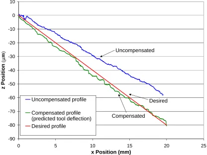
41 Typical results for closed-loop compensation using predicted cutting depth and a non-dynamic cutting force model are shown in Figure 24, with the upper plot representing the uncompensated cutting profile, the middle plot representing the compensated profile, and the lower plot representing the desired profile.

-100 -80 -60 -40 -20 0 20

0 5 10 15 20

x Position (mm)

z Position

(µ

m)

Uncompensated profile

Compensated profile (predicted cutting depth) Desired profile

Uncompensated Compensated

Desired

Figure 24: Experimental profile measurements: predicted depth compensation, linear slotting cut

(55)

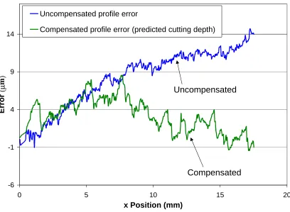
42 location of 8 mm), while maximum error (deflection) in the uncompensated groove reaches a maximum of 14 µm at a location of 18 mm. This equates to a 43% reduction in groove profile error.

-6 -1 4 9 14

0 5 10 15 20

x Position (mm)

Error

(µ

m)

Uncompensated profile error

Compensated profile error (predicted cutting depth)

Uncompensated

Compensated

Figure 25: Experimental profile errors: predicted depth compensation, linear slotting cut

(56)

43 feedback). The axes are enabled, and the experiment begins. Initially, the desired cutting depth is zero. However, there is a measurable force, thus the predicted cutting depth is greater than zero. As a result, the control algorithm commands an initial move away from the workpiece, resulting in significant profile errors at the start of the groove.

Another source of error in the compensated profile involves the theoretical cutting depth vs. normal cutting force relationship (Figure 2). This plot reveals a very small slope at small cutting depths, making it difficult to measure forces at this operating condition due to their intermittent behavior. Thus, a small change in depth has a large effect on the force and limits this method’s accuracy. As the depth increases, the forces become less intermittent (more consistent), resulting in more accurate predictions of cutting depth.

It should be noted that the results shown in Figure 24 and Figure 24 represent the only acceptable results out of approximately 35 experiments conducted using this method of compensation. As a result, the second method of compensation using deflection was investigated to a much greater extent.

5.2.3 P

REDICTED

D

EFLECTION

C

OMPENSATION

(57)

44 -90

-80 -70 -60 -50 -40 -30 -20 -10 0 10

0 5 10 15 20 25

x Position (mm)

z Position

(µ

m)

Compensated profile (predicted tool deflection) Desired profile

Uncompensated

Compensated

Desired

Figure 26: Experimental profile measurements: predicted deflection compensation, linear slotting cut

(58)

45 12.1 12.105 12.11 12.115 12.12 12.125 12.13 12.135 12.14

-4 -2 0 2 4 6 8 10 12 14 16

0 5 10 15 20 25

x Position (mm)

Normal Force,

Fn

(N)

Unfiltered force Maximum force

Maximum filtered force

Maximum force

Unfiltered force

Figure 27: Experimental force measurements: predicted deflection compensation, linear slotting cut

(59)

46

-5 0 5 10 15 20 25

0 5 10 15 20 25

x Position (mm)

Error

(µ

m)

Compensated profile error (predicted tool deflection)

Uncompensated

Compensated

Figure 28: Experimental profile errors: predicted deflection compensation, linear slotting cut

5.3 MODIFIED SINUSOIDAL SLOTTING CUT EXPERIMENTS

Slotting cuts with harmonically varying depth were also made with and without predicted deflection compensation to evaluate the performance of this approach. Trials were not conducted using predicted depth compensation due to problems with initial transients leading to tool breakage.

5.3.1 O

NE

-P

ERIOD

M

ODIFIED

S

INUSOIDAL

P

ROFILE

(60)

47 mm/min with the long tool. The resulting sine wave frequency was 0.52 Hz. As before, groove profiles were measured on the Talysurf profilometer.

A typical set of results is shown in Figure 29, with the upper plot representing the uncompensated cutting profile, the middle plot representing the compensated profile, and the lower plot representing the desired profile.

-90 -80 -70 -60 -50 -40 -30 -20 -10 0 10

0 5 10 15 20 25

x Position (mm)

z Position

(µ

m)

Uncompensated

Compensated

Desired

Figure 29: Experimental profile measurements: predicted deflection compensation, one period sinusoidal slotting cut

(61)

48 Figure 30: Experimental force measurements: predicted deflection compensation, one

period sinusoidal slotting cut

(62)

49 -30

-25 -20 -15 -10 -5 0 5 10 15

0 5 10 15 20 25

x Position (mm)

Error

(µ

m)

Compensated profile error (predicted tool deflection)

Uncompensated

Compensated

(63)

50

5.3.2 T

WO

-P

ERIOD

M

ODIFIED

S

INUSOIDAL

P

ROFILE

Grooves spanning 20 mm with a two-period modified sinusoidal profile and peak depth of 80 µm were programmed, using a spindle speed of 10,000 rpm and a feed rate of 100 mm/min with the long tool. The resulting sine wave frequency was 1.05 Hz. As before, groove profiles were measured on the Talysurf profilometer.

A typical set of results is shown in Figure 32, with the upper plot representing the uncompensated cutting profile, the middle plot representing the compensated profile, and the lower plot representing the desired profile.

-110 -90 -70 -50 -30 -10 10

0 5 10 15 20 25

x Position (mm)

z Position

(µ

m)

Uncompensated

Compensated

Desired

(64)

51 Normal cutting force during a typical one period sinusoidal slotting cut is shown in Figure 33. This cutting force data shows unfiltered force as well as maximum force and filtered maximum force.

12.1 12.105 12.11 12.115 12.12 12.125 12.13 12.135 12.14

-2 0 2 4 6 8 10 12 14

0 5 10 15 20 25

x Position (mm)

Normal Force,

Fn

(N)

Unfiltered force Maximum force

Maximum force

Unfiltered force

Figure 33: Experimental force measurements: predicted deflection compensation, two period sinusoidal slotting cut

(65)

52 -40

-30 -20 -10 0 10 20

x Position (mm)

Error

(µ

m)

Compensated profile error (predicted tool deflection) Uncompensated Compensated

Figure 34: Experimental profile errors: predicted deflection compensation, two period sinusoidal slotting cut

(66)

53 5.4 REPEATABILITY EXPERIMENTS

To evaluate the repeatability of the force feedback deflection compensation results of Figures 25-33, each of these cutting experiments was repeated with different tools. Closed-loop cutting tests were conducted with one tool, then repeated with a different tool on the same workpiece in a different location. The workpiece was not removed from the DTM fixture from one experiment to the next to eliminate misalignment errors.

5.4.1 L

INEAR

S

LOTTING

C

UT

E

XPERIMENTS

(67)

54

-15 -10 -5 0 5 10

0 5 10 15 20 25

x Position (mm)

Error

(µ

m)

Tool 1 compensated profile error (predicted tool deflection)

Tool 2 Tool 1

Figure 35: Experimental profile repeatability errors: predicted deflection compensation, linear slotting cut

Although these results indicate excellent repeatability, profile errors associated with Tool 1 are less than those associated with Tool 2. These variations can be attributed to differences in the workpiece surface before cutting as well as differences in tool stiffness and flute wear from one tool to the next.

(68)

55 This “touching off” the workpiece surface is the same procedure described in section 5.2.2 where a rotating tool was incremented 1 µm in the z-direction toward the workpiece surface while measuring z-force on the load cell. Incremental movements were continued until a force of approximately 0.1 N was seen. At this point it was determined that the surface of the workpiece was found.

5.4.2 O

NE

-P

ERIOD

M

ODIFIED

S

INUSOIDAL

P

ROFILE

(69)

56 -25

-20 -15 -10 -5 0 5 10 15 20

0 5 10 15 20 25

x Position (mm)

Error

(µ

m

)

Tool 2 compensated profile error (predicted tool deflection) Tool 2

Tool 1

Figure 36: Experimental profile repeatability errors: predicted deflection compensation, one period sinusoidal slotting cut

As before, these experimental results reveal excellent correspondence between Tool 1 and Tool 2 in all areas of the groove.

5.4.3 T

WO

-P

ERIOD

M

ODIFIED

S

INUSOIDAL

P

ROFILE

(70)

57

-25 -20 -15 -10 -5 0 5 10 15 20

0 5 10 15 20 25

x Position (mm)

Error

(µ

m)

Tool 2 Tool 1

Figure 37: Experimental profile repeatability errors: predicted deflection compensation, two period sinusoidal slotting cut

(71)

58 5.5 INVESTIGATING PROFILE ERRORS IN SMALL GROOVE

EXPERIMENTS

The causes of profile errors in the small groove experiments are difficult to determine exclusively from Talysurf measurements. To investigate the effects of controller inputs on groove profiles, cuts were made while the following variables and parameters were measured:

• unfiltered cutting force • filtered cutting force

• captured maximum cutting force • encoder position

• filtered tool deflection

• proportional deflection compensation error • derivative deflection compensation error • integral deflection compensation error • axes servo control voltages

• workpiece surface before cutting

Groove profile measurements were made and compared statistically with these acquired measurements. To make these statistical comparisons, cross-correlation coefficients were computed between each gathered variable and the measured groove profiles.

5.5.1 C

ROSS

-C

ORRELATION

C

OEFFICIENTS

(72)

59 positive coefficient means that as one variable increases, the other variable increases, and vice-versa. A negative coefficient indicates that as one variable increases, the other decreases, and vice-versa.

By taking the absolute value of the correlation coefficient, the strength of the relationship between one variable to another is quantified. The closer the absolute value of the correlation coefficient is to unity, the stronger the relationship between the two variables. A correlation coefficient of ±1.0 indicates a perfect linear relationship whereas a correlation coefficient of 0 indicates the absence of a linear relationship.

The cross-correlation coefficient is also the slope of the regression line when both variables have been converted to z-scores. Conversion to a z-score takes place by subtracting out the mean from each raw variable and then dividing the result by the sample standard deviation. The cross-correlation coefficient is invariant to linear transformations, meaning that changing the scale of either variable in the cross-correlation does not affect the cross-cross-correlation coefficient [14].

5.5.2 U

NCOMPENSATED

L

INEAR

S

LOTTING

C

UT

: C

ROSS

-

CORRELATIONS

(73)

60 -2

-1 0 1 2 3 4 5 6 7 8

0 5 10 15 20 25

x Position (mm)

Normal Force,

Fn

(N)

Butterworth filtered force

Maximum captured force

Butterworth filtered force Maximum force

Figure 38: Experimental force measurements: filtered and captured maximum cutting force, uncompensated linear slotting cut

(74)

61 -80

-70 -60 -50 -40 -30 -20 -10 0 10

0 5 10 15 20 25

x Position (mm)

z Position (

µ

m)

Figure 39: Experimental profile measurement: uncompensated linear slotting cut

(75)

62 -5

-4 -3 -2 -1 0 1 2 3

0 5 10 15 20 25

x Position (mm)

z Position (

µ

m)

Figure 40: Experimental workpiece surface profile measurement before cutting

(76)

63 Table 4: Cross-correlation coefficients for uncompensated linear slotting cut

Variable Cross-correlation coefficient

Unfiltered cutting force (dSPACE) -0.4808 Filtered cutting force (dSPACE) -0.5134 Captured maximum force (dSPACE) -0.8634 Filtered tool deflection (PMAC) -0.9693 Z-axis encoder position (PMAC) -0.9989 Proportional error (PMAC) 0.1881 Integral error (PMAC) -0.2892 Derivative error (PMAC) 0.0612 Servo voltage (PMAC) 0.0499 Workpiece surface before cutting -0.2097

The variables with the strongest correlation coefficients are PMAC z-axis encoder position (-0.9989), PMAC filtered tool deflection (-0.9693), and dSPACE captured maximum force (-0.8634). The strong correlation between PMAC encoder position and groove profile is expected; it implies that the tool tip is following axes movement and creating the profile measured on the Talysurf. There is also a strong cross-correlation between PMAC tool deflection and dSPACE captured maximum force with measured groove profile, so it can be concluded that the maximum force during machining has a strong relationship with groove profile created.

5.5.3 C

OMPENSATED

L

INEAR

S

LOTTING

C

UT

: C

ROSS

-

CORRELATIONS

(77)

64

-2 0 2 4 6 8 10

0 5 10 15 20 25

x Position (mm)

Normal Force,

Fn

(N)

Butterwoth filtered force Maximum capture force

Butterworth filtered force Maximum force

Figure 41: Experimental force measurements: Butterworth and maximum force capture, compensated linear slotting cut

(78)

65

-90 -80 -70 -60 -50 -40 -30 -20 -10 0 10

0 5 10 15 20 25

x Position (mm)

z Position (

µ

m)

Figure 42: Experimental profile measurement: compensated linear slotting cut

Table 5: Cross-correlation coefficients for compensated linear slotting cut Variable Cross-correlation coefficient

Unfiltered cutting force (dSPACE) -0.4623

Filtered cutting force (dSPACE) -0.4936

Captured maximum force (dSPACE) -0.8569

Filtered tool deflection (PMAC) -0.9707

Z-axis encoder position (PMAC) -0.9989

Proportional error (PMAC) 0.183

Integral error (PMAC) -0.3003

Derivative error (PMAC) 0.0415

Servo voltage (PMAC) 0.0235

Workpiece surface before cutting -0.2299

Force Feedback Control of Tool Deflection in Miniature Ball End Milling.

ABSTRACT

FORCE FEEDBACK CONTROL OF TOOL

DEFLECTION IN

MINIATURE BALL END MILLING

BIOGRAPHY

ACKNOWLEDGMENTS

TABLE OF CONTENTS

LIST OF TABLES

LIST OF FIGURES

1 INTRODUCTION

2 MODELING TOOL FORCES AND

DEFLECTIONS

z-axis

x-axis

workpiece

spindle

y-axis

n

3 CLOSED-LOOP COMPENSATION OF TOOL

DEFLECTION

( )

( )

3.1.1 A

C

D

P

3.1.2 D

C

D

P

(

)

3.2.1 A

D

P

3.2.2 D

D

P

4 EXPERIMENTAL IMPLEMENTATION

4.2.1 PMAC L

n

{ }

{

}

(

)

β

β

τ

=

T

1

−

τ

Filter output

( )

1

1

ωτ

+

=

a

5 EXPERIMENTAL EVALUATIONS

x

y

z

φ

5.2.1 E

M

F

5.2.3 P

D

C

5.3.1 O

-P

M

S

P

5.3.2 T