HIGHLIGHTED ARTICLE
GENETICS | COMMUNICATIONS
Do Molecular Markers Inform About Pleiotropy?
Daniel Gianola,*,†,‡,1Gustavo de los Campos,§Miguel A. Toro,** Hugo Naya,†† Chris-Carolin Schön,†,‡and Daniel Sorensen‡‡ *Departments of Animal Sciences, Dairy Science, and Biostatistics and Medical Informatics, University of Wisconsin–Madison, Wisconsin 53706,†Department of Plant Sciences Technical University of Munich, Center for Life and Food Sciences, D-85354 Freising-Weihenstephan, Germany,‡Institute of Advanced Study, Technical University of Munich, D-85748 Garching, Germany, §Department of Biostatistics, Michigan State University, East Lansing, Michigan 48824, **Escuela Técnica Superior de Ingenieros
Agrónomos, Universidad Politécnica de Madrid, 20840 Madrid, Spain,††Institut Pasteur de Montevideo, Mataojo 2020, Montevideo 11400, Uruguay, and‡‡Department of Molecular Biology and Genetics, Aarhus University, DK-8000 Aarhus C, Denmark
ABSTRACTThe availability of dense panels of common single-nucleotide polymorphisms and sequence variants has facilitated the study of statistical features of the genetic architecture of complex traits and diseases via whole-genome regressions (WGRs). At the onset, traits were analyzed trait by trait, but recently, WGRs have been extended for analysis of several traits jointly. The expectation is that such an approach would offer insight into mechanisms that cause trait associations, such as pleiotropy. We demonstrate that correlation parameters inferred using markers can give a distorted picture of the genetic correlation between traits. In the absence of knowledge of linkage disequilibrium relationships between quantitative or disease trait loci and markers, speculating about genetic correlation and its causes (e.g., pleiotropy) using genomic data is conjectural.
KEYWORDSgenetic correlation; genomic correlation; genomic heritability; linkage disequilibrium; pleiotropy
T
HE interindividual differences for a trait or disease risk that can be explained by genetic factors, such as trait heritability (h2), the genetic correlation (rG), and thecoher-itability between two traits (rGh1h2), are very important
pa-rameters in quantitative genetic studies of animals, humans, and plants. These quantities play a role in the study of evo-lution due to artificial and natural selection, and knowledge thereof is required for statistical prediction of outcomes in animal and plant breeding as well as medicine. Traditionally, these parameters have been estimated using phenotypes and pedigrees,e.g., family and twin data in human genetics. The availability of dense panels of common single-nucleotide polymorphisms (SNPs) and of sequence data more recently has made it possible to assess kinship among distantly related individuals (Morton et al. 1971; Thompson 1975; Ritland
1996; Lynch and Ritland 1999). This development has opened new opportunities for study of the genetic architec-ture of complex traits and diseases. For instance, Yanget al. (2010) suggested using whole-genome regressions (WGRs) (Meuwissenet al.2001) to assess the proportion of variance of a trait or disease risk that can be explained by a regression of phenotypes on common SNPs or genomic heritability and a related parameter, the“missing heritability.”More recently, WGR models have been extended for the analysis of systems of multiple traits, so the concept ofgenomic correlationalso has entered into the picture (Jia and Jannink 2012; Leeet al. 2012). For instance, Maier et al. (2015) used multivariate WGR models and reported estimates of genetic correlations between psychiatric disorders, and Furlotte and Eskin (2015) presented a methodology that incorporates genetic marker information for the analysis of multiple traits that, according to the authors,“provide fundamental insights into the nature of co-expressed genes.”In a similar spirit, Korteet al.(2012) argued that multitrait-marker-enabled regressions can be useful for understanding pleiotropy. More recently, Bulik-Sullivanet al. (2015) proposed a methodology for“estimating genetic corre-lation”using statistics derived from single-marker genome-wide Copyright © 2015 by the Genetics Society of America
doi: 10.1534/genetics.115.179978
Manuscript received June 26, 2015; accepted for publication July 21, 2015; published Early Online July 23, 2015.
1Corresponding author: Department of Animal Sciences, University of Wisconsin–
association studies (GWAS) and reported estimates of such correlations among 25 human traits.
de los Camposet al.(2015) discussed potential problems that emerge when trying to infer genetic parameters using molecular markers that are imperfectly associated with the gen-otypes at the causal loci. In this paper, the framework described in de los Camposet al.(2015) is extended for the analysis of systems of traits, and it is demonstrated that correlation param-eters inferred using markers can give a distorted picture of the genetic correlation between traits. For instance, it is shown that an analysis based on markers may suggest a genetic correlation when none exists or may fail to detect a genetic correlation when one does exist. It is concluded that in the absence of knowledge about linkage disequilibrium (LD) relationships be-tween quantitative trait loci (QTL) and markers, speculating about genetic correlations, and even more about their causes (e.g., pleiotropy), using genomic data is conjectural.
Theory
To set the stage, consider a single-locus model. In an additive-inheritance framework, a phenotype (y) is regressed on a QTL genotype codeQ(0, 1, and 2 for genotypesaa,Aa, andAA, respectively) according to the linear model
y¼a0þa1QþE (1)
wherea0 anda1 arefixed parameters, andQandEare
in-dependent random variables, the latter representing a model residual. The proportion of phenotypic variance explained by the linear regression onQ, or narrow-sense heritability, is
h2¼ a 2 1SQ
a2 1SQþs2E
where SQ¼varðQÞ is the variance in allelic content, and s2
E ¼varðEÞ is the residual variance. IfQis standardized to a unit variance,
SQ¼1 and h2¼ a 2 1
a2 1þs2E
In quantitative genomic analysis, marker genotypes (X) are used in lieu of the QTL genotypesQbecause the latter are unknown or unobserved. The marker-based or instrumental model, assuming a single marker, is a linear regression on marker genotypeXwith form
y¼a0þb1XþE9 (2)
whereE9is a regression residual. Assuming without loss of generality that bothXandQare in standard deviation units, the marker effect can be shown to beb1¼rQXa1, whererQX is the correlation between the marker and the QTL genotypes, which depends on their LD. In this setting, the proportion of variance of phenotypes explained by the linear regression on the marker, or genomic heritability, is h2
marked¼r 2
QXh2, and
missing heritability is h2
missing¼ ð12r2QXÞh2. Hence, missing
heritability is a function of the LD between the marker and the QTL. Genomic heritability hash2as an upper bound (de
los Camposet al.2015).
The regression model just described can be extended to the analysis of multiple traits affected by multiple QTL. For simplicity, we consider only two markers (X1and X2) and
two QTL (Q1andQ2). A multivariate representation of the
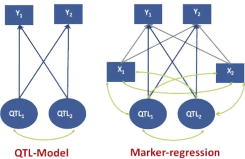
model with an arbitrary number of QTL and markers is pro-vided in the Appendix. Figure 1 depicts a system with two traits, two QTL, and two markers. The left panel represents the regression of the phenotypes on the two QTL, with blue arrows denoting effects from QTL on traits and green arcs denoting LD between QTL. In the QTL model of Figure 1, the genetic correlation is (see Appendix)
rG¼ ffiffiffiffiffiffiffiffiffiffiffiffiffiffiffiffiffiffiffiffiffiffiffiffiffiffiffiffiffiffiffiffiffiffiffiffiffiffiffiffiffi a19SQa2 a19SQa1a29SQa2
q (3)
wherea91¼ ða11 a12Þcontains the effects of QTL 1 and 2
on trait 1, anda92¼ ða21 a22Þcontains the effects of QTL 1
and 2 on trait 2. The variance-covariance matrix between QTL genotypes is given bySQ. If genotypes are standardized,
SQ¼
1 rQ12
rQ21 1
withrQ12 being the correlation between genotypes at QTL 1 and 2. In the QTL model of Figure 1, there are two sources of genetic correlation: pleiotropy (i.e., the same QTL affects more than one trait) and LD between QTL, in this case rep-resented byrQ126¼0. This is well known in quantitative ge-netics (Falconer and Mackay 1996; Knott and Haley 2000).
We now bring the two markers into the picture, as shown in the right panel of Figure 1; here gray arrows are regressions on markers (these are distinct from regressions on QTL genotypes), and arcs denote correlations between genotypes due to LD. In the Appendix, we show that the genomic correlation is
rG;marked¼ a19SQXS
21 X SXQa2
ffiffiffiffiffiffiffiffiffiffiffiffiffiffiffiffiffiffiffiffiffiffiffiffiffiffiffiffiffiffiffiffiffiffiffiffiffiffiffiffiffiffiffiffiffiffiffiffiffiffiffiffiffiffiffiffiffiffiffiffiffiffiffiffiffiffiffiffiffiffiffiffiffiffiffiffiffiffiffiffiffiffiffi
a19SQXS21 X SXQa1
a29SQXS21 X SXQa2
r
(4)
In this expression,SQXis the covariance matrix between QTL and marker genotypes (reflecting marker-QTL LD), andSXis the covariance matrix between marker genotypes, reflecting mutual LD relationships among markers. If markers and gen-otypes are in standard deviation units,
SX¼
1 rX12
rX21 1
and SQX ¼
r
Q1X1 rQ1X2
rQ2X1 rQ2X2
Comparison of the genomic correlation (4) with the genetic correlation (3) indicates that inrrG;marked,SQXS
21
marker-QTL LD patterns conveyed bySQX, and (3) among-marker LD relationships, as conveyed bySX:Notably, one of the sources of genetic correlation,i.e., LD between QTL, as conveyed bySQ, has no effect onrG;marked. Conversely, there
are sources that contribute to the genomic correlation, i.e., marker-marker and marker-QTL LD, that do not enter intorG: Because the sources affecting genetic and genomic corre-lations are distinct, the two parameters can differ greatly. This point is strengthened by considering four stylized cases rep-resented in Figure 2. All the demonstrations supporting the discussion that follows can be found in the Appendix.
Application to Four Situations
Case 1: Independent marker-QTL pairs and absence of pleiotropy (Figure 2, upper-left panel)
This is the simplest case: it consists of two marker-QTL pairs with linkage equilibrium (LE) between pairs but LD within pairs. Each trait is affected by only one QTL; QTL 1 affects trait 1, and QTL 2 affects trait 2. Several simplifications take place here. For instance, because of LE between pairs,rQ1X2¼0, so SQX becomes an identity matrix. Therefore, the genetic co-variance in the numerator of (3) reduces to a19a2. In the
absence of pleiotropy, a19¼ ða11 0Þ and a92¼ ð0 a22Þ
are orthogonal;i.e.,a91a2 ¼0. Therefore, the genetic
corre-lation is null. Furthermore, with LE between pairs, rQ1X2¼rQ2X1 ¼rX1X2 ¼0, leading also to an absence of geno-mic correlation. Thus, in case 1 there is complete agreement between the genomic and genetic correlations: both are null.
Case 2: Phantom correlation (Figure 2, upper-right panel)
The setting is obtained by adding LD between the two markers to case 1. There is no pleiotropy, and the two QTL are in LE, so the genetic correlation is zero (genetically, the system is equiv-alent to case 1). However, because of the LD between markers, SQXS2X1SXQin (4) is no longer diagonal. Consequently, there will be nonzero genomic correlation even in absence of genetic
correlation: markers can induce genomic correlation when traits are genetically uncorrelated—a crucial issue.
Case 3: Missing correlation (Figure 2, lower-left panel)
This scenario illustrates a situation in which the genetic correlation is undetected by the markers and is obtained from case 1 by adding LD between QTL, which, in the absence of pleiotropy, is the only source of genetic correlation between traits. However, SQXS2X1SXQremains diagonal as in case 1. Furthermore, in the absence of pleiotropy,a19a2¼0
(orthog-onality); consequently, rG;marked is null. This example shows
how one source of genetic correlation, namely, LD among QTL, may be completely lost in a genomic analysis.
Case 4: Pleiotropy (Figure 2, lower-right panel)
Here we allow each of the two QTL to affect both traits; otherwise, the setting is as in case 1. Pleiotropy now induces a genetic and a genomic correlation. However,rGandrG;marked
differ in magnitude depending on the patterns of LD and on the magnitude of the pleiotropic effects. To illustrate, we set SX¼SQ¼I2, an identity matrix of order 2; this implies LE
between pairs of QTL and pairs of markers. Further, we take
SQX ¼
0:5 0 0 0:5
or SQX ¼
0:2 0 0 0:8
i.e., homogeneity or heterogeneity of marker-QTL LD, respec-tively. Finally, QTL effects are set to a91¼ ð1 a12Þ and
a92¼ ða21 1Þ, with a12¼a21; this pleiotropic effect was
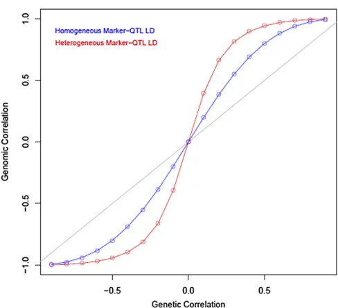
varied over the set of values½20:9;20:8;. . .;0:8;0:9. Fig-ure 3 displays the resulting values of the genomic (vertical axis)vs.genetic (horizontal axis) correlations computed us-ing (3) and (4); the blue curve represents the case where
Figure 2 Two-trait system. Four possible cases of interplay between QTL, markers, and phenotypes. The arrows have the same interpretation as in Figure 1.
marker-QTL LD was the same for both pairs, and the red curve represents the case where LD differed between pairs 1 and 2. Thefigure shows how different patterns of LD induce different magnitudes of genomic and genetic correlations that, however, do not differ in sign in this example.
The genomic covariance does not always preserve the sign of the genetic covariance. Suppose that the two QTL are not pleiotropic but are in LD, with effects a91¼ ða 0Þ and
a92¼ ð0 2aÞand with
SQ¼ 1 1 2 1 2 1 2 6 6 4 3 7 7 5
Using the expression in the numerator of (3), the genetic covariance is
ða 0Þ
1 1 2 1 2 1 2 6 6 4 3 7 7
5ð0 2aÞ9¼ 2a 2
2
which is negative at any nonnull value ofa. Now let the LD relationships between markers and between QTL and markers be such that
SX ¼ 1 4 5 4 5 1 2 6 6 4 3 7 7
5 and SQX ¼ 4 5 0 0 4 5 2 6 6 4 3 7 7 5
The genetic system is such that QTL 1 (QTL 2) is in LD with marker 1 (marker 2), but there is LE between QTL 1 and marker 2 and QTL 2 and marker 1. In the numerator of expression (4),
SQXS21 X SXQ¼
16 9 2 64 45 264 45 16 9 2 6 6 4 3 7 7 5
and the genomic covariance is (64/45)a2, always positive. In
this example, the genomic correlation is 4/5, and the genetic correlation is21/2.
Discussion
In the analysis of systems of complex traits, none of the cases just discussed are likely to“hold”exactly as described, and there is an enormous range of possibilities in terms of within and between marker-QTL genotypes as well as allelic effects sizes and signs. However, the underlying mechanisms that our examples describe are an integral part of the multivariate system involving QTL and markers and are key to an under-standing of why genomic and genetic correlations are distinct parameters. Importantly, there is an ambiguous link between the two parameters. For instance, all or a fraction of the
component of rG that is due to LD among QTL is likely to be missed by an analysis based on markers that are in imper-fect LD with QTL. Also, a fraction of the genetic correlation due to pleiotropy is likely to be missed as a result of imperfect LD between marker and QTL. Finally, LD between markers can create illusory genetic correlations.
What happens if all QTL genotypes are included in the panel of markers, as may be expected if full DNA sequence information is available? Here the sequence can be partitioned into neutral markers (x) and QTL (q) such that for a given individual the genomic data presents asxseq¼ ðx9;q9Þ. Thus,
thesequencecovariance matrix is
varðxseqÞ ¼Sxseq ¼
SX SXQ SQX SQ
(5)
The marked genotype for traitiusing the DNA sequence is
^
Gi¼ai9SQxseqSx2seq1xseq; i¼1;2 (6)
and the genomic or marked covariance is
covðG1^ ;G2Þ ¼^ a91SQxseqS2xseq1SxseqS
21
xseqSxseqQa2 ¼a91SQxseqS2
1
xseqSxseqQa
9
2 (7)
Using partitioned matrix techniques for obtaining the inverse ofSxseqde los Camposet al.(2015) showed that
SQxseqS
21
xseqSxseqQ ¼ ½SQX SQ
0 I
¼SQ (8)
Hence, covðG^1;G^2Þ ¼a91SQa2, the genetic covariance de-fined in equation (A2) in the Appendix. This shows that if the sequence information contains the variants at the causal loci, the marked covariance is equal to the genetic covariance
between traits, and therefore, the genomic correlation is identical to the genetic correlation in that case. However, the genetic correlation depends on allelic frequencies and allele effect sizes at the QTL as well as on LD relationships between the QTL; these parameters, as well as the trait-specific QTL, will still need to be learned properly. Apart fromfi nite-sample-size statistical problems, technical issues such as a large percentage of singleton reads and incomplete gene coverage will complicate matters (Kerr Wall 2009). Hence, when sequence data become available for quantitative genetic studies, unrav-eling the structure of the genetic correlation will not be an easy task, even under the simplifying assumptions of an additive model of inheritance.
In conclusion, multivariate quantitative genetic analysis based on markers can be used to obtain more accurate pre-dictions of complex traits and to estimate genomic correla-tions. However, these parameters cannot always be viewed as genetic correlations because the sources of genetic and geno-mic correlations are distinct. Imperfect LD between markers and QTL produces missing heritability in single-trait analysis; in multivariate models, the problem becomes one of missing, excessive, or spurious (MES) correlation. Care must be exer-cised when interpreting estimates of genomic correlations between complex traits when these traits are assessed by molecular markers as opposed to QTL and even more so when interpreted from a causality perspective. Unfortunately, con-siderably more information is needed than what is now avail-able for a meaningful interpretation of estimates of genomic correlations between pairs of traits when gene action involves many additive QTL. Speculating on the multivariate statistical genetic architecture of complex traits using imperfect instru-ments such as markers seems risky at this time.
Acknowledgments
This work was supported in part by the Wisconsin Agricul-ture Experiment Station and by a U.S. Department of Agriculture Hatch Grant (142-PRJ63CV) to D.G. C.C.S. and D.G. acknowledge support of the Technische Universität München Institute for Advanced Study, funded by the Ger-man Excellence Initiative. G.D.L.C. received support from National Institutes of Health grants R01GM099992 and R01GM101219. M.A.T. wishes to acknowledge funding
from the European Union’s Seventh Framework Programme (KBBE.2013.1.2-10) under grant agreement 61361.
Literature Cited
Bulik-Sullivan, B., H. K. Finucane, V. Anttila, A. Gusev, F. R. Dayet al.
2015 An atlas of genetic correlations across human diseases and traits. bioRxiv doi: http://dx.doi.org/10.1101/014498. de los Campos, G., D. Sorensen, and D. Gianola, 2015 Genomic
heritability: what is it? PLoS Genet. 11: e1005048.
Falconer, D. S., and T. F. C. Mackay, 1996 Introduction to Quan-titative Genetics, Ed. 4. Longmans Green, Harlow, UK.
Furlotte, N. A., and E. Eskin, 2015 Efficient multiple-trait associ-ation and estimassoci-ation of genetic correlassoci-ation using the matrix-variate linear mixed model. Genetics 200: 59–68.
Knott, S. A., and C. S. Haley, 2000 Multitrait least qquares for quantitative trait loci detection. Genetics 156: 899–911. Jia, Y., and J.-L. Jannink, 2012 Multiple trait genomic selection
methods increase genetic value prediction accuracy. Genetics 192: 1513–1522.
Korte, A., B. J. Vilhjálmsson, V. Segura, A. Platt, Q. Long, and M. Nordborg, 2012 A mixed-model approach for genome-wide association studies of correlated traits in structured populations. Nat. Genet. 44: 1066–1071.
Lee, S. H., J. Yang, M. E. Goddard, P. M. Visscher, and N. R. Wray, 2012 Estimation of pleiotropy between complex diseases using single-nucleotide polymorphism-derived genomic relationships and restricted maximum likelihood. Bioinformatics 28: 2540–2542. Lynch, M., and K. Ritland, 1999 Estimation of pairwise
related-ness with molecular markers. Genetics 152: 1753–1766. Maier, R.et al., 2015 Joint analysis of psychiatric disorders increases
accuracy of risk prediction for schizophrenia, bipolar disorder, and major depressive disorder. Am. J. Hum. Genet. 96: 283–294. Meuwissen, T. H. E., B. J. Hayes, and M. E. Goddard,
2001 Prediction of total genetic value using genome-wide dense marker maps. Genetics 157: 1819–1829.
Morton, N. E., S. Yee, D. E. Harris, and R. Lew, 1971 Bioassay of kinship. Theor. Popul. Biol. 2: 507–524.
Ritland, K., 1996 A marker-based method for inferences about quantitative inheritance in natural populations. Evolution 50: 1062–1073.
Thompson, E. A., 1975 The estimation of pairwise relationships. Ann. Hum. Genet. 39: 173–188.
Kerr Wall, P., 2009 Comparison of next generation sequencing technologies for transcriptome characterization. BMC Genomics 10: 347.
Yang, J., B. Benyamin, B. P. McEvoy, S. Gordon, A. K. Henderset al., 2010 Common SNPs explain a large proportion of heritability for human height. Nat. Genet. 42: 565–569.
Appendix
Genetic Correlation
Let G1¼a91q and G2¼a92q be additive genetic values for a pair of traits, where a1 and a2 are vectors of fixed allelic
substitution effects affecting traits 1 and 2, respectively, andqis a random vector indicating the incidence of genotypes at the corresponding QTL. Following de los Camposet al.(2015), the additive genetic variance of trait i is
varðGiÞ ¼ai9SQai; i¼1;2 (A1)
The additive genetic covariance between traits 1 and 2 is then
covðG1;G2Þ ¼a19SQa2 (A2)
whereSQis a covariance matrix between allelic contents at loci affecting the traits. For example, with two QTL (assuming Hardy-Weinberg equilibrium at each of the two QTL),
SQ¼
2p1ð12p1Þ 2D12 2D12 2p2ð12p2Þ
(A3)
wherepjis the frequency of the reference allele at locusj(j =1,2), andD12is the LD statistic between alleles at the two loci. In
scalar notation, (A2) takes the more explicit form
covðG1;G2Þ ¼2½p1ð12p1Þa11a21þp2ð12p2Þa12a22 þ2D12ða12a21þa11a22Þ (A4)
The genetic covariance has a pleiotropy component (thefirst part of the expression) plus a LD component that vanishes if the QTL are in pairwise equilibrium,i.e.,D12¼0:The genetic correlation (Falconer and Mackay 1996) is
rG¼ ffiffiffiffiffiffiffiffiffiffiffiffiffiffiffiffiffiffiffiffiffiffiffiffiffiffiffiffiffiffiffiffiffiffiffiffiffiffiffiffiffiffiffi a19SQa2 a19SQa1a29SQa2
q (A5)
Genomic Correlation
Letxbe a vector of genotypes at p marker loci. The multiple linear regressions ofG1 andG2 onxproduce asfitted values
^
Gi¼a9iSQXS2X1x. The genomic covariance (or marked genetic covariance) is defined as
Cmarked¼covðG1^ ;G2Þ ¼^ a19SQXS2X1SXQa2 (A6)
Thegenomic correlationis
rG;marked¼
Cmarked
ffiffiffiffiffiffiffiffiffiffiffiffiffiffiffiffiffiffiffiffiffiffiffiffiffiffiffiffiffiffiffiffiffiffiffiffiffiffiffiffiffiffiffiffiffiffiffiffiffiffiffiffiffiffiffiffiffiffiffiffiffiffiffiffiffiffiffiffiffiffiffiffiffiffiffiffiffiffiffiffiffiffiffiffi
a19SQXS21 X SXQa1
a29SQXS21 X SXQa2
r (A7)
Interpreting this parameter meaningfully requires knowledge of (1) bivariate QTL effects at all loci, (2) LD relationships between QTL affecting the two traits and the markers via theSQXmatrices, and (3) LD relationships among markers. Unfortunately, only phenotypes, marker genotypes, and LD relationships between markers are observable. Most of the required ingredients in the formula are yet unknown. Importantly, note thatSQ;conveying LD between QTL, does not enter into the genomic correlation.
Independent QTL-Marker Blocks (Case 1 in Figure 2)
Each of two independently segregating QTL is in LD with a marker, with the two markers being in mutual LE, and there is no pleiotropy. Here
SQX ¼SXQ¼SX ¼
1 0
0 1
(A8)
rG¼rG;marked¼ ffiffiffiffiffiffiffiffiffiffiffiffiffiffiffiffiffiffiffiffiffiffiffiffiffiffiffiffiffia19a2 ða19a1Þða29a2Þ
p (A9)
Because there is no pleiotropy,a91a2¼ ða11 0Þ9ð0 a22Þ ¼0, and both correlations are null.
Phantom Correlation (Case 2 in Figure 2)
ConsiderSQXS2X1SXQin (A6), where (given standardized genotypes)
SQX ¼ "
rQ1X1 rQ1X2
rQ2X1 rQ2X2 #
¼ "
rQ1X1 0 0 rQ2X2
#
S21 X ¼
"
1 rX1X2
rX1X2 1 #21
¼ 1
12r2X1X2 "
1 2rX1X2 2rX1X2 1
#
SXQ¼ "
rQ1X1 0 0 rQ2X2
#
(A10)
Then
SQXS21 X SXQ¼
1 12r2
X1X2 "
r2
Q1X1 2rQ1X1rQ2X2rX1X2 2rQ1X1rQ2X2rX1X2 r2Q2X2
#
(A11)
The off-diagonals of this matrix are nonnull, so a genomic correlation will arise when there is no genetic correlation.
Missing Correlation (Case 3 in Figure 2)
Because the markers are in LE,S2X1 is an identity matrix, so
SQXS21
X SXQ ¼SQXSXQ¼ "
r2 QX 0
0 r2
QX #
Therefore, in the absence of pleiotropy,Cmarkedin (A6) and, thus,rG;markedwill be null no matter what the value of the genetic
correlation.
Pleiotropy (Case 4 in Figure 2)