Gene Level Meta-Analysis of Quantitative Traits by Functional Linear Models

(1)

GENETICS | INVESTIGATION

Gene Level Meta-Analysis of Quantitative Traits by

Functional Linear Models

Ruzong Fan,*,1_{Yifan Wang,* Michael Boehnke,}†_{Wei Chen,}‡_{Yun Li,}§_{Haobo Ren,** Iryna Lobach,}†† and Momiao Xiong‡‡

*Biostatistics and Bioinformatics Branch, Division of Intramural Population Health Research, Eunice Kennedy Shriver National

Institute of Child Health and Human Development, National Institutes of Health, Bethesda, Maryland 20892,†Department of

Biostatistics, School of Public Health, University of Michigan, Ann Arbor, Michigan 48109,‡Division of Pulmonary Medicine,

Allergy, and Immunology, University of Pittsburgh Medical Center, Pittsburgh, Pennsylvania 15224,§Department of Genetics,

Department of Biostatistics, University of North Carolina, Chapel Hill, North Carolina 27599, **Regeneron Pharmaceuticals,

Basking Ridge, New Jersey 07920,††Division of Biostatistics, Department of Epidemiology and Biostatistics, University of California,

San Francisco, California 94185, and‡‡Human Genetics Center, University of Texas, Houston, Texas 77225

ABSTRACTMeta-analysis of genetic data must account for differences among studies including study designs, markers genotyped, and covariates. The effects of genetic variants may differ from population to population,i.e., heterogeneity. Thus, meta-analysis of combining data of multiple studies is difﬁcult. Novel statistical methods for meta-analysis are needed. In this article, functional linear models are developed for meta-analyses that connect genetic data to quantitative traits, adjusting for covariates. The models can be used to analyze rare variants, common variants, or a combination of the two. Both likelihood-ratio test (LRT) andF-distributed statistics are introduced to test association between quantitative traits and multiple variants in one genetic region. Extensive simulations are performed to evaluate empirical type I error rates and power performance of the proposed tests. The proposed LRT andF-distributed statistics control the type I error very well and have higher power than the existing methods of the meta-analysis sequence kernel association test (MetaSKAT). We analyze four blood lipid levels in data from a meta-analysis of eight European studies. The proposed methods detect more signiﬁcant associations than MetaSKAT and theP-values of the proposed LRT and F-distributed statistics are usually much smaller than those of MetaSKAT. The functional linear models and related test statistics can be useful in whole-genome and whole-exome association studies.

KEYWORDSmeta-analysis; rare variants; common variants; association mapping; quantitative trait loci; complex traits; functional data analysis

M

ETA-ANALYSIS is a statistical method to combine mul-tiple studies for a uniﬁed analysis and it plays an important role in genetic studies (de Bakker et al. 2008; Zeggini and Ioannidis 2009; Cantor et al.2010; Evangelou and Ioannidis 2013). One obvious advantage of meta-analysis is that the sample size is large (Liuet al.2014). Therefore, meta-analysis should lead to more signiﬁcant results. It is argued that most of the reported complex disease associations came from

large-scale meta-analysis of genome-wide association studies (GWASs) (Zeggini and Ioannidis 2009; Evangelou and Ioannidis 2013; Liu et al. 2014). Therefore, there has been great in-terest in developing novel statistical methods to perform GWAS meta-analysis (Ioannidis et al.2007; Huet al. 2013; Liuet al.2014). Meta-analysis combines studies with differ-ent study designs. The genotype data and covariates may vary from study to study. Moreover, the effects of genetic variants in different populations may not be the same,i.e., the hetero-geneity (Tang and Lin 2014). Thus, meta-analysis of combin-ing data of multiple studies is difﬁcult. Novel statistical methods for meta-analysis are needed.

The statistical methods for meta-analysis fall into two classes: (1) single genetic variant-based approaches and (2) gene-based variant analysis approaches. The single genetic variant approaches only use one genetic variant at a time and are usually based onﬁxed-effect linear regression models for

Manuscript received January 21, 2015; accepted for publication June 5, 2015; published Early Online June 9, 2015.

Supporting information is available online at www.genetics.org/lookup/suppl/

doi:10.1534/genetics.115.178343/-/DC1.

(2)

quantitative traits,x2_{-tests, or score tests for qualitative traits.}

The single genetic variant approaches are mainly applied to analyze common variants (Zegginiet al.2008; Hindorffet al.

2009; Stahlet al.2010). Gene-based approaches use multiple genetic variants in genetic regions in the analysis and can analyze rare variants, common variants, or combinations of the two. Developing gene-based approaches for association analysis is a major area of interest. A few recent studies have targeted analysis of rare variants.

Three types of tests are available for gene-based associ-ation analysis of complex diseases. The ﬁrst type is burden tests that are based on collapsing rare variants in a genetic region to be a single variable that is then used to test for association with the phenotypes (Li and Leal 2008; Madsen and Browning 2009; Morris and Zeggini 2010; Price et al.

2010). Burden tests were built to analyze rare variants by aggregating statistics of multiple rare variants for an analysis.

The second type is variance-component tests such as the sequence kernel association test (SKAT) and its optimal uniﬁed version (SKAT-O) (Lee et al. 2012). In Lee et al.

(2012), it was shown that SKAT-O has higher power than some burden tests, such as the combined collapsing and multivariate method (Li and Leal 2008) and the nonparametric weighted sum test (Madsen and Browning 2009). By extend-ing SKAT and SKAT-O to perform meta-analysis, Lee et al.

(2013) developed meta-analysis SKAT and SKAT-O (MetaSKAT and MetaSKAT-O) to carry out meta-analysis for rare variants in multiple studies. Both SKAT and MetaSKAT are score tests based on mixed-effect models.

The third type is tests based onﬁxed-effect models that include (1) traditional additive effect models that are well studied (Cordell and Clayton 2002; Fan and Xiong 2002; Fan et al. 2006) and (2) functional regression models as shown in our previous research (Luoet al. 2012; Fanet al.

2013, 2014; Wanget al.2015). Note that functional regres-sion models areﬁxed-effect models, which extend traditional population genetics models to analyze multiple genetic var-iants and can analyze rare varvar-iants, common varvar-iants, or combinations of the two. For individual studies with small and moderate sample sizes, functional linear models (FLMs) were proposed to analyze quantitative traits. The FLMs lead tox2_{-score tests and}_F_{-distributed statistics, which are more}

powerful than SKAT and SKAT-O while controlling type I error correctly (Luo et al. 2012; Fan et al. 2013; Wang

et al.2015). For dichotomous traits, generalized FLMs were developed to perform gene-based association analysis (Fan

et al.2014).

In functional regression models, we treat multiple genetic variants of an individual as a realization of an underlying stochastic process (Ross 1996). Therefore, the genome of an individual in a chromosome region is a continuum of se-quence data rather than discrete observations. The genome of an individual is viewed as a stochastic function that contains both genetic position and linkage disequilibrium (LD) infor-mation of the genetic markers. In short, the functional

regres-sion models have a number of advantages: (1) the genetic effects at the major gene locus are modeled as ﬁxed effects, which ﬁt traditional population genetics theory and modern genetic data very well; (2) the models fully utilize LD and genetic position information; and (3) the models test for a joint effect of genetic variants, including both common and rare.

It is worth of noting that SKAT and SKAT-O were found to perform better than C-alpha (Nealeet al.2011) and burden tests (Li and Leal 2008; Madsen and Browning 2009; Morris and Zeggini 2010; Price et al.2010). Hence, FLMs are po-tentially very powerful in association analysis of complex quantitative traits. The superior performance of the FLMs motivates us to extend them to perform meta-analysis.

In this article, FLMs are developed for meta-analysis of multiple studies to connect genetic data to quantitative traits, adjusting for covariates. We allow that different studies may have different environmental factors/covariates, and genetic variants may differ among studies. The effects of genetic variants may differ from population to population,

i.e., heterogeneity. This makes it possible for us to build

ﬂexible models for meta-analysis of multiple studies. We assume that individual genotype data are available from all studies.

Both likelihood-ratio test (LRT) and F-distributed statis-tics of FLMs are introduced to test association between quantitative traits and multiple genetic variants in one gene region. Extensive simulations are performed to evaluate the empirical type I error rates and power performance of the proposed models and tests. The proposed methods are ap-plied to analyze four blood lipid levels in data from meta-analysis of eight European studies.

Materials and Methods

Consider a meta-analysis withLstudies in a genomic region. For the ℓth study, we assume that there are nℓ individuals who are sequenced in the genomic region atmℓvariants. We assume that themℓvariants are located with ordered genetic positions 0#tℓ1,⋯,tℓmℓ#T: To make the notation

sim-pler, we normalized the region½tℓ1;Tto be [0, 1]. For theith

individual in theℓth study, letyℓidenote her/his quantitative

trait,Gℓi¼ ðXℓiðtℓ1Þ;⋯;XℓiðtℓmℓÞÞ9denote her/his genotypes of

the mℓ variants, and Zℓi¼ ðzℓi1;⋯;zℓicℓÞ9 denote her/his cℓ

covariates. Hereafter, 9 denotes the transpose of a vector or matrix. For the genotypes, we assume that XℓiðtℓjÞ

ð¼0;1;2Þ is the number of minor alleles of the individual

iat thejth variant.

General functional linear model

In this section, we view theith individual’s genotype data as a genetic variant function (GVF) XℓiðtÞ;t2 ½0;1: Note that

the sample includes nℓdiscrete realizations or observations

Gℓi¼ ðXℓiðtℓ1Þ;⋯;XℓiðtℓmℓÞÞ9 of the human genome. By using

the genetic variant information G_ℓi; we may estimate the

related GVF XℓiðtÞ;which is discussed below. To relate the

(3)

y_ℓi¼aℓ0þZℓ9iaℓþ

Z 1

0

X_ℓiðtÞbℓðtÞdtþeℓi;

ℓ¼1;2;⋯;L; i¼1;2;⋯;n_ℓ; (1)

whereaℓ0 is the overall mean,aℓ¼ ðaℓ1;⋯;aℓcℓÞ9is a cℓ31

column vector of regression coefﬁcients of covariates,b_ℓðtÞis the genetic effect of GVF XℓiðtÞ at the position t, andeℓi is

an error term. For each ℓ and i, the error term eℓi is

nor-mally distributed with a mean of zero and a variance s2 e:

Moreover, eℓ1;⋯;eℓnℓ are independent variables, and

eℓ¼ ðeℓ1;⋯;eℓnℓÞ9 are independent vectors of variables,

ℓ¼1;2;⋯;L:Similar to the GVF, we assume that the ge-netic effectb_ℓðtÞis a function of the genetic positiont.

Expansion of genetic effect function: The genetic effect

functionb_ℓðtÞis assumed to be smooth. One may expand it by B-spline or Fourier basis functions. Formally, let us expand the genetic effect function b_ℓðtÞ by a series ofKb basis functions cðtÞ ¼ ðc1ðtÞ;⋯;cKbðtÞÞ9asbℓðtÞ ¼cðtÞ9bℓ;

where b_ℓ¼ ðb_ℓ1;⋯;bℓKbÞ9 is a vector of coefﬁcients

bℓ1;⋯;bℓKb: We consider two types of basis functions:

(1) the B-spline basis, ckðtÞ ¼BkðtÞ;k¼1;⋯;Kb;and (2) the Fourier basis, c1ðtÞ ¼1;c2rþ1ðtÞ ¼sinð2prtÞ; and

c2rðtÞ ¼cosð2prtÞ;r¼1;⋯;ðKb21Þ=2:Here for the

Four-ier basis, Kb is taken as a positive odd integer (de Boor 2001; Ramsay and Silverman 2005; Ferraty and Romain 2010; Horváth and Kokoszka 2012).

Estimation of genetic variant function: To estimate the

genetic variant functions XℓiðtÞ from the genotypes Gℓi;

we use an ordinary linear square smoother (Ramsay and Silverman 2005; Ramsayet al.2009; Fanet al.2013). Let fkðtÞ;k¼1;⋯;K;be a series of Kbasis functions, such as

the B-spline basis and Fourier basis functions. Denote fðtÞ ¼ ðf1ðtÞ;⋯;fKðtÞÞ9:LetFdenote themℓby theK

ma-trix containing the valuesfkðtℓjÞ;wherej21;⋯;mℓ:Using

the discrete realizationsGℓi¼ ðXℓiðtℓ1Þ;⋯;Xℓiðtℓm_ℓÞÞ9;we may

estimate the GVF XℓiðtÞ; using an ordinary linear square

smoother as follows (Ramsay and Silverman 2005, Chap. 4):

^

X_ℓiðtÞ ¼ ðXℓiðtℓ1Þ;⋯;XℓiðtℓmℓÞÞF

h

F9Fi21fðtÞ: (2)

Revised functional linear model: We expand XℓiðtÞ by the

ordinary linear square smoother. Assume that the genetic effect b_ℓðtÞ is expanded by a series of basis functions as bℓðtÞ ¼ ðc1ðtÞ;⋯;cKbðtÞÞðbℓ1;⋯;bℓKbÞ9¼cðtÞ9bℓ: Replacing XℓiðtÞ in the functional linear model (1) by X^ℓiðtÞ in (2)

andb_ℓðtÞby the expansion, we have a revised linear regres-sion model

yℓi¼aℓ0þZℓ9iaℓþ

ðXℓiðtℓ1Þ;⋯;XℓiðtℓmℓÞÞF

h

F9Fi21

Z 1

0 f

ðtÞc9ðtÞdt

bℓþeℓi¼aℓ0þZℓ9iaℓþW_ℓ9ib_ℓþe_ℓi;

(3)

whereWℓ9i¼ ðXℓiðtℓ1Þ;⋯;XℓiðtℓmℓÞÞF½F9F2

1R1

0fðtÞc9ðtÞdt:In

the above revised regression model, one needs to calculate

F½F9F21

and R₀1fðtÞc9ðtÞdt to get Wℓi: In the statistical

packages R or Matlab, there are readily available codes to calculate them (Ramsayet al.2009).

b-smooth only functional linear models

Model (1) is a theoretical FLM in functional data analysis literature (Ramsay and Silverman 2005). For analysis of dense genetic data, one may use a simpliﬁed model,

yℓi¼aℓ0þZℓ9iaℓþ

Xmℓ

j¼1

XℓiðtℓjÞbℓðtℓjÞ þeℓi;

ℓ¼1;2;⋯;L; i¼1;2;⋯;n_ℓ; (4)

whereb_ℓðtℓjÞis the genetic effect at the positiontℓjfor theℓth

study, and the other terms are similar to those in the general model (1). In the above model, the integration term

R1

0 XℓiðtÞb_ℓðtÞdtin model (1) is replaced by the summation

termPmℓ

j¼1XℓiðtℓjÞb_ℓðtℓjÞ:It turns out that model (4) performs

very similarly to model (1) in real data analysis and simu-lations due to high resolution of genotype data (Fan et al.

2013, 2014; Wanget al.2015).

In model (4),b_ℓðtℓjÞis introduced as the genetic effect at

the positiontℓj:We assume that the genetic effect function

bℓðtÞ is a function of the genetic position t. Therefore, bℓðtℓjÞ;j¼1;2;⋯;mℓ;are the values of functionbℓðtÞat the

mℓgenetic positions. The genetic effect function bℓðtÞ is as-sumed to be smooth. One may expand it by B-spline or Fourier basis functions as above. Replacing b_ℓðtℓjÞ by the

expansion, model (4) can be revised as

"

Xmℓ

j¼1

X_ℓiðtℓjÞ

c1ðtℓjÞ;⋯;cK_bðtℓjÞ

#

3 bℓ1;⋯;bℓKb

9_þ_e

ℓi¼aℓ0þZℓ9iaℓþWℓ9ibℓþeℓi; (5)

where Wℓ9i¼Pjm¼ℓ1XℓiðtℓjÞðc1ðtℓjÞ;⋯;cKbðtℓjÞÞ: In model (4)

and its revised version (5), we use the raw genotype data

Gℓi¼ ðXℓiðtℓ1Þ;⋯;XℓiðtℓmℓÞÞ9 directly in the analysis. The

ge-netic effect functionb_ℓðtÞ is assumed to be smooth. Hence, the models are calledb-smooth only.

Traditional additive effect models

Traditionally, an additive effect model can be used to analyze the relation between the trait and themℓvariants in theℓstudy as

Xmℓ

j¼1

X_ℓiðtℓjÞb_ℓjþeℓi;

ℓ¼1;2;⋯;L; i¼1;2;⋯;nℓ; (6)

(Fan and Xiong 2002; Fan et al. 2006), where b_ℓj is the

(4)

models (1) and (4). There is only one difference between model (4) and model (6);i.e., the genetic effect coefﬁcients bℓj in model (6) do not depend on the genetic positiontℓj;

whileb_ℓðtℓjÞin model (4) depend on the genetic positiontℓj:

The genetic effect coefﬁcientsb_ℓj in model (6) are discrete,

whileb_ℓðtℓjÞin model (4) are the values of functionb_ℓðtÞat

the genetic positions tℓj;j¼1;2;⋯;mℓ:

The number of parameters of model (6) can be large, and so it may not be powerful. Moreover, model (6) can model only the LD between the trait and each of the genetic variants as well as the pairwise LD between the genetic variants, but it cannot model higher-order LD among the genetic variants (Fan and Xiong 2002; Fan et al.2006). In spite of the potential drawbacks, model (6) can be easily implemented by standard statistical software such as R, and we use it to make comparison with models (1) and (4). To facilitate the computation in applications, the QR decomposition can be applied to the genotype data to remove the redundancy if the number of genetic variants is large, i.e., to decompose the genotype matrix into the product of an orthogonal matrix Q and a triangular matrix R via Gram-Schmidt process.

One common feature of models (1), (4), and (6) is that they are allﬁxed-effect models. The novel part of models (1) and (4) is that we may revise them to be models (3) and (5) by functional data analysis techniques, in which the num-bersKandKbof basis functions do not depend on the num-bers mℓof genetic variants. This makes models (1) and (4) able to conveniently analyze high-dimension genetic variant data.

LRT and F-distributed statistics

We consider the revised regression models (3) and (5) as usual multiple linear regressions. First, assume that the genetic effects among the L studies are different/ heterogeneous. To test the association between the ge-netic variants and the quantitative trait, the null hypothesis is H0 :b_ℓ¼ ðb_ℓ1;⋯;bℓKbÞ9¼0;ℓ¼1;⋯;L: By using the

standard statistical approach, we may test the null H0 :b_ℓ¼0 by a LRT and an F-distributed statistics. The

LRT statistic is x2 _{distributed with}_LK

b d.f. and is denoted as Het-LRT. The F-distributed statistic’s degrees of freedom (d.f.) are ðLKb;PLℓ¼1ðnℓ2KbÞ21Þ (Weisberg 2005). The F-distributed statistic is denoted as Het-F.

If the genetic effects are homogeneous, i.e., b_ℓ¼ ðbℓ1;⋯;bℓKbÞ9¼b¼ ðb1;⋯;bKbÞ9;ℓ¼1;⋯;L; we may test

the association between the genetic variants and the quantita-tive trait by testing a simpliﬁed null H0 :b¼ ðb1;⋯;bKbÞ9¼

0:Again, a LRT and anF-distributed statistics can be used to test the null H0 :b¼ ðb1;⋯;bKbÞ9¼0:TheF-distributed statistic

has d.f. ðKb;PLℓ¼1nℓ2Kb21Þ: The F-distributed statistic is

denoted as Hom-F. The LRT is x2 distributed withKb d.f. and is denoted as Hom-LRT.

For the additive effect model (6), the null hypothesis of no association between the genetic variants and the quan-titative trait is H0 :b_ℓ¼ ðb_ℓ1;⋯;bℓmℓÞ9¼0;ℓ¼1;⋯;L;

un-der an assumption of heterogeneous genetic effect. The corresponding LRT statistic is x2 _{distributed with} PL

ℓ¼1mℓ

d.f., and the corresponding F-distributed statistic has d.f. as ðPL_ℓ_¼1mℓ;

PL

ℓ¼1ðnℓ2mℓÞ21Þ: The tests are denoted as

Het-LRT and Het-F.

Assume that each individual of the L studies is se-quenced at the same variants located at 0#t1,⋯,tm

and som1¼⋯¼mℓ¼m: In addition, assume that the ge-netic effects are homogenous; i.e., b_ℓ¼ ðb_ℓ1;⋯;bℓmℓÞ9¼

b¼ ðb1;⋯;bmÞ9:Then, model (6) is simpliﬁed as

Xm

j¼1

X_ℓiðtjÞbjþeℓi;

ℓ¼1;2;⋯;L; i¼1;2;⋯;n_ℓ: (7)

The null hypothesis of no association between the gen-etic variants and the quantitative trait is H0 :b¼

ðb1;⋯;bmÞ9¼0:The corresponding LRT statistic isx2

dis-tributed with m d.f., and the corresponding F-distributed statistic has d.f. as ðm;PL_ℓ_¼₁n_ℓ2m21Þ: The tests are denoted as Hom-LRT and Hom-F.

Parameters of functional data analysis

In the data analysis and simulations, we used the functional data analysis procedure in the statistical package R. We use two functions in library fda of the R package as follows to create basis:

basis = create.bspline.basis(norder = order, nbasis = bbasis) basis = create.fourier.basis(c(0,1), nbasis = fbasis).

The three parameters were taken as order = 4, bbasis = 15, fbasis = 25 in all data analysis. In the simulations, the three parameters were taken as order = 4, bbasis = 15, fbasis = 21 for the heterogeneous genetic effect model and order = 4, bbasis = 15, fbasis = 25 for the homogeneous genetic effect model. Speciﬁcally, the order of B-spline basis was 4, the number of basis functions of B-spline was

K¼Kb¼15 and the number of Fourier basis functions was K¼Kb¼21 for the heterogeneous genetic effect model, and similarly the number of basis functions of B-spline was K¼Kb¼15 and the number of Fourier basis functions was K¼Kb¼25 for the homogeneous genetic effect model.

To make sure that the results are valid and stable, we tried a wide range of parameters: (1) 10#K¼Kb#23 for the heterogeneous genetic effect model and (2) 10#

K¼Kb#29 for the homogeneous genetic effect model. The results are similar to each other.

Results

Meta-analysis of lipid traits in eight European cohorts

(5)

and one from Germany (DIAGEN). The two Norwegian cohorts are combined as one study for a joint analysis. The genotype data were from Metabochip genotyping, which was designed toﬁne map regions that have been associated to metabolic traits (Altshuleret al.2010). For each cohort, 54,741 genetic variants were genotyped.

For our analysis, we utilized the existing literature as a reference for gene selection and found that 22 gene regions wereﬁne mapped (Liuet al.2014). We used Builder Mar. 2006 (NCBI36/hg18) to determine gene positions and 5 kb was used to extend the gene region on each side of a gene. The summary of 22 genes and the number of genetic variants in each gene region are given in Supporting Information,Table S1.

Four lipid traits were analyzed: high-density lipoprotein (HDL) levels, low-density lipoprotein (LDL) levels, trigly-cerides (TG), and total cholesterol (CHOL). The sample sizes for each trait are provided inTable S2. For each trait, inverse normal rank transformation was performed to make sure that normality is valid. For all studies except for METSIM, age, sex, and type 2 diabetes status were used as covariates. For METSIM, age and type 2 diabetes status were used as covariates since no female was included in the study. A signiﬁcance threshold of P,3:131026 was taken from Liu et al. (2014) (corresponding to 0.05/16,153 and allowing for the number of genes tested therein). In addi-tion, a covariate for Norwegian study origin was created, since the two Norwegian cohorts were analyzed jointly.

Table 1 reports results of association analysis of the eight European cohorts by homogeneous LRT (LRT), Hom-MetaSKAT-O, and Hom-MetaSKAT; and Table 2 reports results by heterogeneous LRT (Het-LRT), Het-MetaSKAT-O, and Het-MetaSKAT. The results of Hom-F and Het-F are reported in Table S3 and Table S4. At the signiﬁcance

threshold ofP,3:131026_;_{we observe the following}

asso-ciations by both Hom-LRT and Hom-F of functional regres-sion models (3) and (5): (1) at theLPLfor HDL levels; (2) at theAPOB,APOE,LDLR, andPCSK9for LDL levels; (3) at the

APOE and LPL for TG levels; and (4) at theAPOB,APOE,

HNF1A, and LDLR for CHOL levels. Hom-MetaSKAT and Hom-MetaSKAT-O detect the following associations: (1) at the APOE, LDLR, and PCSK9 for LDL levels and (2) at the

APOEandLDLRfor CHOL levels.

By both Het-LRT and Het-F of functional regression models (3) and (5) shown in Table 2 and Table S4, we observe the following associations: (1) at theAPOB,APOE,

CDC123,CDKAL1,CDKN2B,FTO,HNF1A,LDLR,OASL,PCSK9, andTSPAN8for LDL levels; (2) at theLPLfor TG levels; and (3) at the APOB, APOE, CDC123, CDKAL1, CDKN2B, FTO,

HNF1A,IDE,JAZF1,KIF11,LDLR,MTNR1B,OASL,PCSK9, and TSPAN8 for CHOL levels. MetaSKAT and Het-MetaSKAT-O detect the following associations: (1) at theAPOE

andLDLRfor LDL levels and (2) at theAPOEfor CHOL levels. In addition to the results of functional regression models (3) and (5), MetaSKAT, and MetaSKAT-O, Table 1, Table 2,

Table S3, andTable S4report the results of the traditional additive effect models (6) and (7). The additive effect mod-els (6) and (7) detect more association signals than Meta-SKAT and MetaMeta-SKAT-O, but less than the functional regression models (3) and (5).

Generally, theP-values of Hom-LRT in Table 1 are slightly smaller than those of Hom-F inTable S3, and theP-values of Het-LRT in Table 2 are slightly smaller than those of Het-F in

Table S4. Hence, the LRT statistics are slightly more power-ful than the F-distributed statistics. In addition, Het-LRT and Het-F detect more association signals than Hom-LRT and Hom-F. Overall, theP-values of Hom-MetaSKAT-O and Hom-MetaSKAT are bigger than those of Hom-LRT and Table 1 Association analysis of lipid traits in eight European cohorts by homogeneous likelihood-ratio tests (Hom-LRT), Hom-MetaSKAT-O, and Hom-MetaSKAT

P-values of Hom-LRT

Basis of both GVF andbℓðtÞ Basis ofb-smooth only P-values of Hom-

Meta-Traits Gene B-spline basis Fourier basis B-spline basis Fourier basis Additive model (7) SKAT SKAT-O

HDL LPL 3:0631026 ₆_:₁₃₃₁₀29 ₃_:₆₄₃₁₀26 ₆_:₇₅₃₁₀27 ₈_:₃₂₃₁₀24 ₁_:₀₈₃₁₀23 ₁_:₂₁₃₁₀23

LDL APOB 3:3531029 ₇_:₅₀₃₁₀24 ₅_:₇₆₃₁₀28 ₁_:₈₇₃₁₀24 ₃_:₈₄₃₁₀25 ₁_:₆₃₃₁₀22 ₂_:₅₁₃₁₀22

APOE 1:27310287 ₃_:₄₂₃₁₀291 ₄_:₀₇₃₁₀283 ₄_:₄₂₃₁₀290 ₄_:₂₃₃₁₀289 ₁_:₁₈₃₁₀243 ₆_:₆₇₃₁₀244

LDLR 8:25310215 ₁_:₆₇₃₁₀214 ₅_:₀₉₃₁₀215 ₉_:₂₄₃₁₀214 ₇_:₁₄₃₁₀217 ₁_:₀₃₃₁₀210 ₂_:₉₄₃₁₀210

PCSK9 2:2931026 ₅_:₃₆₃₁₀210 ₁_:₆₅₃₁₀26 ₁_:₂₇₃₁₀27 ₂_:₃₅₃₁₀217 ₆_:₁₈₃₁₀27 ₂_:₀₀₃₁₀26

TG APOE 4:9531026 ₆_:₆₁₃₁₀26 ₅_:₁₃₃₁₀27 ₁_:₉₀₃₁₀26 ₁_:₃₇₃₁₀26 ₁_:₃₄₃₁₀23 ₂_:₅₉₃₁₀23

LPL 2:03310211 ₇_:₄₈₃₁₀213 ₂_:₆₀₃₁₀211 ₄_:₂₃₃₁₀214 ₅_:₅₂₃₁₀27 ₁_:₇₈₃₁₀25 ₁_:₇₇₃₁₀25

CHOL APOB 1:9831028 7:8831023 2:1931027 1:1631024 6:6031028 6:1731022 1:0031021

APOE 2:48310253 ₃_:₁₂₃₁₀253 ₁_:₅₂₃₁₀248 ₁_:₃₆₃₁₀251 ₁_:₉₈₃₁₀251 ₉_:₀₈₃₁₀223 ₂_:₁₅₃₁₀222

HNF1A 1:0831021 1:8431022 8:9431023 2:8431026 1:7431021 1:8931021 2:7731021

LDLR 8:10310211 ₈_:₄₉₃₁₀210 ₈_:₅₉₃₁₀210 ₆_:₆₈₃₁₀29 ₂_:₀₇₃₁₀212 ₃_:₄₃₃₁₀27 ₁_:₁₅₃₁₀26 The associations that attain a threshold signiﬁcance ofP,3:131026_{are boldface (Liu}_{et al.}_{2014). The results of}_“_{Basis of both GVF and}_b

ℓðtÞ”were based on smoothing

both GVF and genetic effect functionsbℓðtÞof model (3), the results of“Basis ofb-smooth only”were based on the smoothingbℓðtÞonly approach of model (5), the results

(6)

Hom-F, and theP-values of Het-MetaSKAT-O and Het-MetaSKAT are bigger than those of Het-LRT and Het-F. Therefore, MetaSKAT is less sensitive than the proposed LRT and

F-distributed statistics.

When we analyze the data sets separately for each study, signiﬁcant association is detected only atAPOEfor LDL and CHOL, levels for a few studies and atLDLRfor CHOL levels in the study of METSIM (Table S5). No signiﬁcant associa-tion is detected for TG and HDL levels in any separate study. TheP-values of separate analysis inTable S5are much big-ger than those of meta-analysis in Table 1, Table 2, Table S3, andTable S4. Thus, it is more advantageous to perform meta-analysis of multiple studies.

A simulation study

To evaluate the performance of the proposed methods, we carried out simulation analyses for two cases: (1) the causal variants are all rare and (2) the causal variants are both rare and common. Simulations were performed for three scenar-ios listed in Table 3 (Leeet al.2013). For scenarios 1 and 2, we used the European-like (EUR) sequence data used in Lee

et al. (2012). For scenario 3, we used both the EUR and

African–American-like (AA) sequence data. Specifically, the EUR sequence data were generated using COSI’s (available at:http://www.broadinstitute.org/sfs/) calibrated best-fit models, and the generated European haplotypes mimick Centre d’Etude du Polymorphisme Humain (CEPH) Utah individuals with ancestry from northern and western Europe in terms of site frequency spectrum and LD pattern (figure 4 in Schaffneret al.2005; International HapMap Consortium 2007). Similarly, the AA sequence data mimick individuals with a 20:80 mixture of Europeans and Africans, together with parameters calibrated to model realistic demographic history (including bottleneck, population expansion, and mi-gration events). The EUR sequence data included 10,000 chromosomes covering 1-Mb regions, and the AA sequence data included 45,000 chromosomes covering 0.1-Mb regions. Genetic regions of 3-kb length were randomly se-lected in the simulations for type I error and power calculations.

Type I error simulations:To evaluate the type I error rates

of the proposed models and tests, we generated phenotype data sets by using the model

Table 2 Association analysis of lipid traits in eight European cohorts by heterogeneous likelihood-ratio tests (Het-LRT), Het-MetaSKAT-O, and Het-MetaSKAT

P-values of the Het-LRT

Basis of both GVF andbℓðtÞ Basis ofb-smooth only P-values of

Het-Meta-Traits Gene B-spline basis Fourier basis B-spline basis Fourier basis Additive model (6) SKAT SKAT-O

LDL APOB 5:05310211 ₄_:₇₂₃₁₀28 ₅_:₀₅₃₁₀211 ₄_:₇₂₃₁₀28 ₃_:₃₇₃₁₀26 ₇_:₆₁₃₁₀22 ₁_:₄₀₃₁₀21

APOE 1:59310281 ₁_:₁₁₃₁₀279 ₁_:₅₉₃₁₀281 ₁_:₁₁₃₁₀279 ₇_:₄₇₃₁₀279 ₂_:₂₃₃₁₀233 ₁_:₂₈₃₁₀238

CDC123 1:7231026 ₃_:₁₉₃₁₀28 ₁_:₇₂₃₁₀26 ₃_:₁₉₃₁₀28 ₅_:₀₄₃₁₀23 ₂_:₅₄₃₁₀21 ₄_:₁₉₃₁₀21

CDKAL1 5:0631027 ₄_:₇₈₃₁₀28 ₅_:₀₆₃₁₀27 ₄_:₇₈₃₁₀28 ₆_:₄₁₃₁₀23 ₃_:₇₄₃₁₀21 ₅_:₈₁₃₁₀21

CDKN2B 6:6431027 ₉_:₈₂₃₁₀26 ₆_:₆₄₃₁₀27 ₁_:₂₀₃₁₀25 ₁_:₅₁₃₁₀25 ₇_:₄₆₃₁₀21 ₉_:₂₀₃₁₀21

FTO 2:0831026 ₁_:₀₅₃₁₀25 ₂_:₀₈₃₁₀26 ₁_:₀₅₃₁₀25 ₃_:₃₂₃₁₀24 ₁_:₁₁₃₁₀22 ₂_:₂₃₃₁₀22

HNF1A 6:22310211 ₅_:₄₁₃₁₀28 ₆_:₂₂₃₁₀211 ₂_:₂₆₃₁₀28 ₈_:₀₇₃₁₀211 ₁_:₃₁₃₁₀21 ₂_:₂₆₃₁₀21

LDLR 6:0931029 ₁_:₄₀₃₁₀29 ₈_:₆₁₃₁₀29 ₁_:₂₃₃₁₀29 ₂_:₂₉₃₁₀29 ₄_:₂₇₃₁₀27 ₄_:₉₃₃₁₀27

OASL 1:1331027 ₄_:₁₇₃₁₀26 ₁_:₁₃₃₁₀27 ₅_:₉₈₃₁₀26 ₈_:₀₆₃₁₀26 ₁_:₂₀₃₁₀21 ₈_:₈₁₃₁₀22

PCSK9 4:9531029 ₈_:₉₈₃₁₀213 ₄_:₉₅₃₁₀29 ₂_:₀₁₃₁₀211 ₄_:₅₄₃₁₀212 ₉_:₀₃₃₁₀24 ₂_:₀₉₃₁₀23

TSPAN8 6:9431029 ₁_:₆₃₃₁₀210 ₇_:₉₄₃₁₀211 ₁_:₀₃₃₁₀210 ₁_:₆₃₃₁₀210 ₆_:₄₇₃₁₀22 ₁_:₂₂₃₁₀21

TG LPL 1:2631025 8:5031027 ₁_:₂₆₃₁₀25 ₈_:₅₀₃₁₀27 ₄_:₄₄₃₁₀25 ₃_:₃₈₃₁₀26 ₆_:₃₀₃₁₀26

CHOL APOB 1:38310212 ₃_:₃₇₃₁₀210 ₁_:₃₈₃₁₀212 ₃_:₃₇₃₁₀210 ₁_:₁₅₃₁₀29 ₆_:₀₄₃₁₀22 ₁_:₁₂₃₁₀21

APOE 2:47310255 ₁_:₃₆₃₁₀252 ₂_:₄₇₃₁₀255 ₁_:₃₆₃₁₀252 ₁_:₆₀₃₁₀252 ₂_:₇₆₃₁₀220 ₃_:₀₈₃₁₀222

CDC123 2:2931026 ₁_:₄₀₃₁₀26 ₂_:₂₉₃₁₀26 ₁_:₄₀₃₁₀26 ₁_:₀₃₃₁₀22 ₇_:₁₃₃₁₀21 ₈_:₉₇₃₁₀21

CDKAL1 4:6231028 ₂_:₇₀₃₁₀29 ₄_:₆₂₃₁₀28 ₂_:₇₀₃₁₀29 ₁_:₁₁₃₁₀24 ₁_:₁₇₃₁₀21 ₂_:₀₆₃₁₀21

CDKN2B 1:8231027 ₁_:₃₆₃₁₀26 ₁_:₈₂₃₁₀27 ₆_:₃₈₃₁₀27 ₁_:₂₀₃₁₀26 ₁_:₁₇₃₁₀21 ₆_:₃₉₃₁₀21

FTO 2:8531027 ₁_:₄₈₃₁₀26 ₂_:₈₅₃₁₀27 ₁_:₄₈₃₁₀26 ₅_:₃₇₃₁₀27 ₉_:₈₄₃₁₀23 ₁_:₉₉₃₁₀22

HNF1A 4:32310211 ₈_:₉₈₃₁₀29 ₄_:₃₂₃₁₀211 ₈_:₃₁₃₁₀29 ₃_:₆₄₃₁₀210 ₄_:₃₃₃₁₀21 ₅_:₃₈₃₁₀21

IDE 6:1231025 ₁_:₃₇₃₁₀26 ₆_:₁₂₃₁₀25 ₁_:₃₇₃₁₀26 ₇_:₅₂₃₁₀25 ₂_:₃₀₃₁₀21 ₃_:₈₆₃₁₀21

JAZF1 2:2031026 ₃_:₉₅₃₁₀26 ₂_:₂₀₃₁₀26 ₃_:₉₅₃₁₀26 ₆_:₈₉₃₁₀24 ₉_:₅₂₃₁₀22 ₁_:₇₁₃₁₀21

KIF11 9:7531027 ₆_:₆₉₃₁₀27 ₉_:₇₅₃₁₀27 ₆_:₆₉₃₁₀27 ₁_:₂₆₃₁₀25 ₂_:₇₇₃₁₀21 ₄_:₄₀₃₁₀21

LDLR 2:4231026 ₃_:₉₁₃₁₀28 ₃_:₂₂₃₁₀26 ₃_:₇₃₃₁₀28 ₇_:₁₅₃₁₀28 ₄_:₇₇₃₁₀24 ₂_:₂₈₃₁₀25

MTNR1B 6:8031027 ₅_:₉₁₃₁₀27 ₆_:₈₀₃₁₀27 ₁_:₃₄₃₁₀27 ₅_:₇₁₃₁₀27 ₄_:₁₆₃₁₀22 ₇_:₄₈₃₁₀22

OASL 1:1131027 ₉_:₂₇₃₁₀28 ₁_:₁₁₃₁₀27 ₁_:₄₂₃₁₀27 ₉_:₆₆₃₁₀28 ₃_:₁₁₃₁₀21 ₅_:₀₆₃₁₀22

PCSK9 1:8731025 2:0931026 1:8731025 8:1731026 5:4531027 1:8931022 3:7231022

TSPAN8 1:11310210 ₂_:₂₉₃₁₀213 ₃_:₁₅₃₁₀213 ₂_:₈₉₃₁₀213 ₂_:₇₀₃₁₀213 ₉_:₄₃₃₁₀22 ₁_:₇₄₃₁₀21 The associations that attain a threshold signiﬁcance ofP,3:131026_{are boldface (Liu}_{et al.}_{2014). The results of}_“_{Basis of both GVF and}_b

ℓðtÞ”were based on smoothing both GVF

and genetic effect functionsbℓðtÞof model (3), the results of“Basis ofb-smooth only”were based on the smoothingbℓðtÞonly approach of model (5), the results of“Additive model

(7)

y_ℓi¼0:5zℓi1þ0:5zℓi2þeℓi; ℓ¼1;2;3; (8)

for scenario 1 in Table 3 and

y1i¼0:5z1i1þe1i

y2i¼0:5z2i1þ0:5z2i2þe2i

y3i¼0:5z3i1þ0:5z3i2þ0:5z3i3þe3i

(9)

for scenarios 2 and 3 in Table 3, wherezℓi1is a dichotomous

covariate taking values 0 and 1 with an equal probability of 0.5,zℓi2 andzℓi3 are continuous covariates from standard

nor-mal distributions Nð0;1Þ; and eℓi follows a standard normal

distributionNð0;1Þ:To obtain genotype data, 3-kb subregions were randomly selected in the 1-Mb region of EUR-like data and the 0.1-Mb region of AA-like data. The ordered genotypes were these SNPs in the 3-kb subregions. Note that the trait values are not related to the genotypes, and so the null hy-pothesis holds. The sample sizes of the data sets were taken as 1600 (study 1), 2200 (study 2), and 3200 (study 3), respec-tively. The simulation settings are summarized in Table 3. For each sample size combination, 106 _{phenotype–genotype data}

sets were generated toﬁt the proposed models and to calculate the test statistics and relatedP-values. Then, an empirical type I error rate was calculated as the proportion of 106 _P_-values

that were smaller than a given a-level (i.e., 0.05, 0.01 and 0.001, 0.0001, respectively).

Empirical power simulations: To evaluate the power

performance of the proposed tests, we simulated data sets under the alternative hypothesis by randomly selecting 3-kb subregions to obtain causal variants for the phenotype values as follows. Once a 3-kb subregion was selected, a subset ofp

causal variants located in the 3-kb subregion was then ran-domly selected to obtain ordered genotypesðgðt1Þ;⋯;gðtpÞÞ:

Then, we generated the quantitative traits by

y_ℓi¼0:5zℓi1þ0:5zℓi2þbℓi1gðt1Þ þ⋯þbℓipg

tp

þeℓi;

ℓ¼1;2;3;

for scenario 1 and for scenarios 2 and 3,

y1i¼0:5z1i1þb1i1gðt1Þ þ⋯þb1ipg

tp

þe1i

y2i¼0:5z2i1þ0:5z2i2þb2i1gðt1Þ þ⋯þb2ipg

tp

þe2i

y3i¼0:5z3i1þ0:5z3i2þ0:5z3i3 þb3i1gðt1Þ þ⋯þb3ipg

tp

þe3i;

where zℓij and eℓi are the same as in the type I error

models (8) and (9), and the b’s are the additive effect for the causal variants deﬁned as follows. We used jb_ℓijj ¼cℓjlog10ðMAFjÞj=2;where MAFjwas the minor allele

frequency (MAF) of the jth variant. Three genetic effect scenarios were used to perform power calculations: (1) all causal variants had positive effects, (2) 20%/80% causal variants had negative/positive effects, and (3) 50%/50% causal variants had negative/positive effects. As in Lee

et al. (2013), four different settings were considered: 5%, 10%, 20%, and 50% of variants in the 3-kb subregion are chosen as causal variants. When 5%, 10%, 20%, and 50% of the variants were causal, two parameter settings of genetic effects were considered for cℓ :(1) homogeneous and (2) heterogeneous (Table 4). In the homogeneous case, the ge-netic effects are the same for the three studies; i.e.,

c1¼c2 ¼c3:In the heterogeneous case, the genetic effects

are different for the three studies; i.e., c2¼c1þ0:15; c3¼c120:15:For each setting, 1000 data sets were

simu-lated to calculate the empirical power as the proportion of

P-values that are smaller than a givena¼0:0001 level. The homogeneous settings of genetic effect are taken from Lee

et al.(2013).

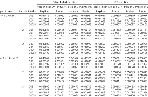
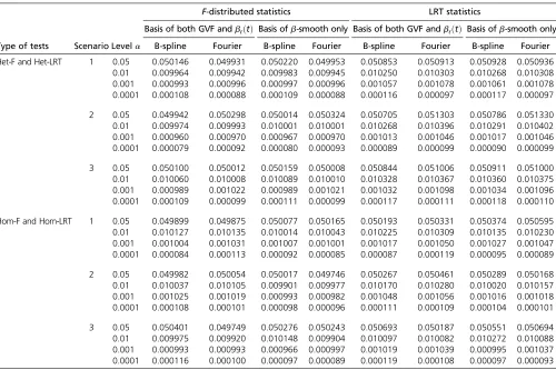
Type I error simulation results: The empirical type I error

rates are reported in Table 5 when the causal variants are only rare and in Table 6 when the causal variants are both rare and common. For each entry of empirical type I error rates, we generated 106 _{data sets. Results of four different}

a¼0:05; 0:01; 0:001;and 0.0001 levels are reported. For both the proposed F-distributed tests and LRT statistics of the functional linear models, all empirical type I error rates are around the nominala-levels for both B-spline basis and Fourier basis (columns 4–11 of Table 5 and Table 6). There-fore, both the F-distributed tests and LRT statistics of the functional linear models controlled type I error rates cor-rectly for all scenarios at all signiﬁcance levels. The func-tional linear models and relatedF-distributed tests and LRT statistics can be useful in both genome and whole-exome association studies.

Statistical power results: We compared the power

perfor-mance of the proposed tests with MetaSKAT and MetaBurden tests based on the simulated COSI sequence data. The empirical power levels of the proposed LRT statistics at the Table 3 Simulation study settings

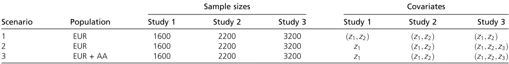
Sample sizes Covariates

Scenario Population Study 1 Study 2 Study 3 Study 1 Study 2 Study 3

1 EUR 1600 2200 3200 ðz1;z2Þ ðz1;z2Þ ðz1;z2Þ

2 EUR 1600 2200 3200 z1 ðz1;z2Þ ðz1;z2;z3Þ

3 EUR + AA 1600 2200 3200 z1 ðz1;z2Þ ðz1;z2;z3Þ

(8)

a¼0:0001 level are plotted in Figure 1, Figure 2, Figure 3, Figure 4,Figure S1,Figure S2,Figure S3, andFigure S4. In the legends of all the ﬁgures, “GVF&Beta, B-sp” (or

“GVF&Beta, F-sp”) means that both genetic variant function and genetic effect functionbðtÞwere smoothed by B-spline (or Fourier) basis functions, and “Beta, B-sp” (or “Beta, F-sp”) means that only the genetic effect functionbðtÞwas smoothed by B-spline (or Fourier) basis functions (i.e.,b-smooth only). Moreover, the results of“Het-MetaSKAT,” “Het-MetaSKAT-O,”

“Hom-MetaSKAT,” “Hom-MetaSKAT-O,”and the metaburden weighted sum test (MetaBurdenWST) using the R package MetaSKAT are reported for power comparison (Madsen and Browning 2009; Leeet al.2012, 2013).

In Figure 1, Figure 2, Figure 3, and Figure 4, the results of

“Hom-LRT”are reported, where the LRT statistics are con-structed using the homogeneous effect model that assumes b1¼b2¼b3:InFigure S1,Figure S2,Figure S3, andFigure S4, the results of “Het-LRT” are reported, where the LRT statistics are constructed using the heterogeneous effect model in which the regression coefﬁcients b1;b2; and b3

are different from each other. In Figure 1, Figure 2,Figure S1, andFigure S2, the simulated data are generated under the assumption of homogeneous genetic effect; and in Fig-ure 3, FigFig-ure 4, Figure S3, and Figure S4, the simulation data are generated under the assumption of heterogeneous genetic effect (Table 4).

The proposed homogeneous LRT statistics (Hom-LRT) of the functional linear models have higher power than that of MetaSKAT and MetaSKAT-O in Figure 1, Figure 2, Figure 3, and Figure 4. The heterogeneous LRT statistics (Het-LRT) of the functional linear models also have higher power than that of MetaSKAT and MetaSKAT-O inFigure S1,Figure S2,

Figure S3, andFigure S4, except for a few cases inFigure S2

when 20% or 50% of variants were causal. Therefore, the proposed LRT statistics of the functional linear models have superior performance in most cases. InFigure S2, the simu-lated data were generated using the homogeneous genetic effect (Table 4), but the data were analyzed by the hetero-geneous effect model and the test is Het-LRT. Thus, it is not strange that there is power loss by Het-LRT inFigure S2.

As shown in Leeet al. (2013, p. 44), MetaSKAT-O takes the minimum P-value of a weighted average of MetaSKAT and the metaburden weighted sum test for a range of r values over ½0;1 and the metaburden weighted sum test

corresponds tor¼1 in the construction of SKAT-O. There-fore, the power of MetaBurdenWST is generally lower than that of MetaSKAT-O. This is consistent with the results of Leeet al.(2013).

In Figure 1 and Figure 2, the simulated data were gen-erated under the assumption of homogeneous genetic effect and the data were analyzed by the homogeneous effect model and the test was Hom-LRT. In Figure S3andFigure S4, the simulated data were generated under the assump-tion of heterogeneous genetic effect and the data were an-alyzed by the heterogeneous effect model and the test was Het-LRT. Therefore,“correct models”were used in analyz-ing the simulated data in Figure 1, Figure 2,Figure S3, and

Figure S4, in which the proposed LRT statistics have signif-icantly higher power levels than those of MetaSKAT. Even when “wrong models”were used to analyze the simulated data in Figure 3, Figure 4, Figure S1, and Figure S2, the empirical power levels of the proposed LRT statistics were much higher than those of MetaSKAT in most cases except a few inFigure S2.

In total, we compared four LRT statistics of the functional linear models in each graph: two are based on B-spline basis functions, and two are based on Fourier basis functions. In the two LRT statistics to use B-spline (or Fourier) basis functions, one is to smooth both the genetic variant functions and the genetic effect functionbðtÞ, and the other is to smooth only the genetic effect function bðtÞ (i.e., b-smooth only). Generally, the four LRT statistics of the functional linear models have similar power. The power lev-els ofb-smooth only are almost identical to those of smooth-ing both the genetic variant functions and the genetic effect functionbðtÞby B-spline basis (or Fourier basis). Thus, the tests do not strongly depend on whether the genotype data are smoothed or not. In addition, the LRT statistics do not strongly depend on which basis functions are used.

In addition to the LRT statistics, we calculated the empirical power levels of the F-distributed statistics, which provide very similar empirical power levels as the LRT statistics (data not shown).

Discussion

In this article, FLMs are developed to perform gene-level meta-analysis of quantitative traits for a combined analysis Table 4 Simulation parameter settings

Causal %

Genetic effect StudyðcℓÞ 5 10 20 50

Homogeneous 1ðc1Þ 0.475 0.375 0.25 0.175

2ðc2Þ 0.475 0.375 0.25 0.175

3ðc3Þ 0.475 0.375 0.25 0.175

Heterogeneous 1ðc1Þ 0.475 0.375 0.25 0.175

2 (c2) 0:475þ0:15 0:375þ0:15 0:25þ0:15 0:175þ0:15

3ðc3Þ 0:47520:15 0:37520:15 0:2520:15 0:17520:15

(9)

of multiple studies. By using functional data analysis techniques, the theoretical FLMs (1) and (4) are trans-formed to be traditional multiple linear regressions (3) and (5) (de Boor 2001; Ramsay and Silverman 2005; Ramsay

et al. 2009; Ferraty and Romain 2010; Horváth and Kokoszka 2012). The null hypothesis of association is tested by LRT and F-distributed statistics. We show that the pro-posed LRT andF-distributed statistics control the type I error very well and have higher empirical power levels than the existing methods such as MetaSKAT and MetaBurdenWST in most simulations. By applying the proposed methods to an-alyze four blood lipid levels in data from a meta-analysis of eight European studies, it is found that the proposed meth-ods detect more signiﬁcant association than MetaSKAT and MetaSKAT-O, and theP-values of the proposed LRT andF -distributed statistics are usually much smaller than those of MetaSKAT and MetaSKAT-O.

One reason that the proposed functional linear models perform better is that SKAT and MetaSKAT do not model LD among genetic markers sufﬁciently. Spe-ciﬁcally, the test statistic of SKAT is given by Qs¼

ðy2p^Þ9GWWG9ðy2p^Þ ¼Pmj¼1w2jf

Pn

i¼1gijðyi2p^iÞg

2_;

where y¼ ðy1;⋯;ynÞ9 is the trait value column vector, G¼

ðG1;⋯;GnÞ9 is the n3m genotype matrix, and W¼

diagðw1;⋯;wmÞ is anm3mdiagonal weight matrix using

the notations of Leeet al.(2012). LetSj¼

Pn

i¼1gijðyi2p^iÞ:

Then, Sj is the score test statistic for testing H0 :bj¼0 in

the single genetic variant model with only the jth genetic variant

logitðpiÞ ¼a0þZ9aþgijbj:

Thus, Sj models the pairwise LD between the jth genetic

variant and the trait locus. Note that QS¼

Pm

j¼1w2jS2j is

a weighted summation of the squared score test statistics

Sj: Therefore, the test statistics of SKAT and MetaSKAT

model pairwise LD only between each individual marker and the trait locus, while the LD among genetic markers are not modeled.

Note that Lee et al. (2012) used dichotomous traits to present the test statisticQs;but the formulation ofQsis also

the same for continuous traits or survival traits (Chenet al.

2014). SKAT and MetaSKAT were constructed as score tests on the variance component parameter for the genetic ran-dom variations in linear or logistic mixed-effects models. The reason that the regression coefﬁcients of genetic terms were assumed to be random in the models of SKAT and MetaSKAT is that the number of genetic variants in a genetic Table 5 Empirical type I error rates ofF-distributed statistics and LRT statistics at differenta-levels based on 106_{simulated data sets,}

when the causal variants are only rare

F-distributed statistics LRT statistics

Basis of both GVF andbℓðtÞ Basis ofb-smooth only Basis of both GVF andbℓðtÞ Basis ofb-smooth only

Type of tests Scenario Levela B-spline Fourier B-spline Fourier B-spline Fourier B-spline Fourier

Het-F and Het-LRT 1 0.05 0.049876 0.049922 0.050093 0.049924 0.050611 0.050895 0.050819 0.050916

0.01 0.009932 0.010006 0.009987 0.010029 0.010173 0.010407 0.010225 0.010422

0.001 0.000991 0.000974 0.001000 0.000971 0.001055 0.001056 0.001065 0.001056

0.0001 0.000089 0.000097 0.000091 0.000095 0.000094 0.000107 0.000097 0.000105

2 0.05 0.049838 0.050189 0.050077 0.050194 0.050546 0.051163 0.050789 0.051164

0.01 0.009944 0.009848 0.009998 0.009851 0.010239 0.010251 0.010305 0.010253

0.001 0.001024 0.001021 0.001036 0.001025 0.001079 0.001082 0.001090 0.001088

0.0001 0.000094 0.000101 0.000094 0.000102 0.000103 0.000118 0.000105 0.000118

3 0.05 0.049886 0.050002 0.050081 0.049940 0.050593 0.050934 0.050789 0.050906

0.01 0.009948 0.010084 0.009989 0.010090 0.010255 0.010454 0.010294 0.010446

0.001 0.000981 0.001044 0.000985 0.001035 0.001029 0.001104 0.001033 0.001098

0.0001 0.000106 0.000093 0.000108 0.000097 0.000116 0.000105 0.000118 0.000108

Hom-F and Hom-LRT 1 0.05 0.049834 0.049795 0.049948 0.049906 0.050131 0.050221 0.050240 0.050337

0.01 0.009932 0.009901 0.009896 0.010018 0.010050 0.010062 0.010012 0.010216

0.001 0.000987 0.001039 0.001030 0.000996 0.001000 0.001070 0.001054 0.001022

0.0001 0.000091 0.000102 0.000077 0.000108 0.000098 0.000104 0.000078 0.000112

2 0.05 0.050140 0.050340 0.050057 0.050050 0.050459 0.050784 0.050349 0.050475

0.01 0.009995 0.010131 0.010001 0.009911 0.010103 0.010308 0.010141 0.010078

0.001 0.000965 0.001029 0.000977 0.000998 0.000984 0.001061 0.001001 0.001031

0.0001 0.000095 0.000106 0.000085 0.000092 0.000099 0.000111 0.000088 0.000097

3 0.05 0.049900 0.049757 0.050173 0.049742 0.050201 0.050213 0.050453 0.050180

0.01 0.010043 0.010068 0.010047 0.009950 0.010157 0.010260 0.010161 0.010138

0.001 0.001025 0.001002 0.001010 0.001017 0.001045 0.001023 0.001035 0.001060

0.0001 0.000090 0.000121 0.000098 0.000118 0.000092 0.000128 0.000100 0.000125

The results of“Basis of both GVF andbℓðtÞ”were based on smoothing both GVF and genetic effect functionsbℓðtÞof model (3), and the results of“Basis ofb-smooth only”

(10)

region is usually large. For instance, there are 660 genetic variants in the region of theKCNQ1gene in data of Euro-pean cohorts, Table S1. Due to a large number of genetic terms in a regression model, it is hard to estimate the ge-netic effects of all gege-netic variants by ordinary ﬁxed-effect regression models. By making the regression coefﬁcients of the genetic terms to be random, the theory of mixed models was used to build the test statistics of SKAT and MetaSKAT (Leeet al.2012, 2013).

In association studies, association between phenotypic traits and major gene loci is tested. If the number of causal genetic variants at a major gene locus is very large and each causal variant makes a small contribution to the phenotype, the assumption of mixed models will be satisﬁed and SKAT and MetaSKAT should perform well (Fisher 1918). On the other hand, if the number of causal genetic variants at a ma-jor gene locus is not large and the contribution of a few causal variants to the phenotype is reasonably large,ﬁ xed-effect models should work well. In our simulation studies and real data analysis, the proposed functional linear mod-els perform better than SKAT and MetaSKAT in most cases. Thus, the mixed models of SKAT and MetaSKAT could be statistically convenient and attractive but not necessarily

bi-ologically reasonable. We argue that theﬁxed-effect models are useful in most cases. In practice, it makes sense to per-form analysis by both the ﬁxed- and mixed-effect models and make a comparison, and this can be readily done using our R codes and SKAT and MetaSKAT packages.

The proposed FLMs are ﬁxed-effect models that can analyze large numbers of genetic variants and extend traditional population genetics models naturally. Unlike other methods such as SKAT or MetaSKAT and burden tests that treat genetic variants as discrete variables, FLMs treat the genetic variant data as continuous stochastic functions or realizations of an underlying stochastic process (Ross 1996). Since genetic variant data are treated as functions, the genetic effects are modeled as functions. One advantage of treating genetic variant data as functions is that the LD information and genetic positions of genetic variant data are contained in the genetic variant functions. The regres-sion coefﬁcients of genetic terms in the models of SKAT and MetaSKAT do not depend on the genetic position, while our genetic effect function depends on the genetic position and is actually a function of genetic position. Hence, the pro-posed models can fully utilize LD and genetic position information.

Table 6 Empirical type I error rates ofF-distributed statistics and LRT statistics at differenta-levels based on 106_{simulated data sets,}

when the causal variants are both rare and common

F-distributed statistics LRT statistics

Basis of both GVF andbℓðtÞ Basis ofb-smooth only Basis of both GVF andbℓðtÞ Basis ofb-smooth only

Type of tests Scenario Levela B-spline Fourier B-spline Fourier B-spline Fourier B-spline Fourier

Het-F and Het-LRT 1 0.05 0.050146 0.049931 0.050220 0.049953 0.050853 0.050913 0.050928 0.050936

0.01 0.009964 0.009942 0.009983 0.009945 0.010250 0.010303 0.010268 0.010308

0.001 0.000993 0.000996 0.000997 0.000996 0.001057 0.001078 0.001061 0.001078

0.0001 0.000108 0.000088 0.000109 0.000088 0.000116 0.000097 0.000117 0.000097

2 0.05 0.049942 0.050298 0.050014 0.050324 0.050705 0.051303 0.050786 0.051330

0.01 0.009974 0.009993 0.010001 0.010001 0.010268 0.010396 0.010291 0.010402

0.001 0.000960 0.000970 0.000967 0.000970 0.001013 0.001046 0.001017 0.001046

0.0001 0.000079 0.000092 0.000080 0.000093 0.000089 0.000099 0.000090 0.000099

3 0.05 0.050100 0.050012 0.050159 0.050008 0.050844 0.051006 0.050911 0.051000

0.01 0.010060 0.010008 0.010089 0.010010 0.010328 0.010367 0.010360 0.010375

0.001 0.000989 0.001022 0.000989 0.001021 0.001032 0.001098 0.001034 0.001096

0.0001 0.000109 0.000099 0.000111 0.000099 0.000117 0.000111 0.000118 0.000110

Hom-F and Hom-LRT 1 0.05 0.049899 0.049875 0.050077 0.050165 0.050193 0.050331 0.050374 0.050595

0.01 0.010127 0.010135 0.010014 0.010043 0.010225 0.010309 0.010135 0.010230

0.001 0.001004 0.001031 0.001007 0.001001 0.001017 0.001050 0.001027 0.001047

0.0001 0.000084 0.000113 0.000092 0.000085 0.000087 0.000119 0.000095 0.000089

2 0.05 0.049982 0.050054 0.050017 0.049746 0.050267 0.050461 0.050289 0.050168

0.01 0.010037 0.010105 0.009901 0.009977 0.010170 0.010280 0.010020 0.010157

0.001 0.001025 0.001019 0.000993 0.000982 0.001048 0.001056 0.001016 0.001018

0.0001 0.000108 0.000101 0.000098 0.000096 0.000111 0.000109 0.000104 0.000101

3 0.05 0.050401 0.049749 0.050276 0.050243 0.050693 0.050187 0.050551 0.050694

0.01 0.009975 0.009920 0.010148 0.009904 0.010097 0.010082 0.010272 0.010088

0.001 0.000993 0.000993 0.000966 0.000997 0.001019 0.001039 0.000995 0.001037

0.0001 0.000116 0.000100 0.000097 0.000089 0.000119 0.000108 0.000097 0.000093

The results of“Basis of both GVF andbℓðtÞ”were based on smoothing both GVF and genetic effect functionsbℓðtÞof model (3), and the results of“Basis ofb-smooth only”

(11)

(12)

The functional linear models (1) and (4) are built to analyze data of multiple studies that may have different covariates and genetic variants. If all studies are genotyped at the same markers and they have the same covariates, then models (1) and (4) are the same as those of Fan et al.

(2013) if the genetic effects are homogeneous; i.e., b1ðtÞ ¼⋯¼bLðtÞ: In reality, the homogeneity assumption

may not be valid in which case the functional linear models (1) and (4) are not a trivial extension of the models of Fan

(13)

(14)

more association signals are detected by Het-LRT and Het-F than by Hom-LRT and Hom-F, reﬂecting the presence of heterogeneity of the genetic effects.

In single studies with sample sizes of#1000, LRT sta-tistics of FLMs were found to inﬂate the type I error rates

(15)

and their empirical power levels are similar when the sam-ple sizes of combined multisam-ple studies are large. In Fan

et al.(2013), the LRT statistics were found to have correct type I error rates when the sample sizes were $1500 in a single study. Therefore, the conclusion that both LRT and

F-distributed statistics can be used for large sample meta-analysis in this article is consistent with the result of Fan

et al.(2013).

The proposed method requires full genotype data;i.e., we assume that individual genotype data are available from all studies. One reason is that we have this type of data in the eight European cohorts. The proposed ap-proach is more powerful than MetaSKAT and MetaSKAT-O when genotype data are available from all studies, and the proposed method cannot meta-analyze summary sta-tistics while MetaSKAT can. If summary stasta-tistics of func-tional regression models are available from different studies only using Fan et al. (2013), it is still an open question if those statistics can be used to meta-analyze the data of multiple studies. Note that the functional regressions are simply ordinary regressions after revising the theoretical functional models by functional data anal-ysis techniques, and so the strategy of usual meta-analanal-ysis would be useful. Hence, it should be possible to use results from functional regression models for a meta-analysis across cohorts. However, the details are still waiting for further work.

With the rapid advance of high-throughput sequencing technologies (Mardis 2008; Ansorge 2009), more sequenc-ing data from large cohorts will be collected and more meta-analyses will be performed in different populations. Association analysis has been increasingly carried out to identify risk or protective genetic variants of complex traits. It is important to develop powerful and efﬁcient statistical methods to test for associations. Our meta-analysis FLMs provide an effective approach for the as-sociation analysis of complex traits.

Acknowledgments

Two anonymous reviewers and the editors, Chiara Sabatti and Gary Churchill, provided very good and insightful comments for us to improve the manuscript. We greatly thank the European cohort investigators for letting us analyze the data and use them as examples. Heather M. Stringham and Tanya M. Teslovich kindly sent us the data of the European cohorts and patiently answered many ques-tions about the cohorts, which we greatly appreciated. We thank Seunggeun Lee for sending us the simulation program of SKAT and sequence data generated by Yun Li using the program COSI. This study utilized the high-performance computational capabilities of the Biowulf Linux cluster at the National Institutes of Health (http://biowulf.nih.gov). The methods proposed in this article are implemented by using the procedure of functional data analysis (fda) in the statistical package R. The R codes for data analysis and

simulations are available at http://www.nichd.nih.gov/ about/org/diphr/bbb/software/fan/Pages/default.aspx. This study was supported by the Intramural Research Pro-gram of the Eunice Kennedy Shriver National Institute of Child Health and Human Development, National Institutes of Health (NIH) (Ruzong Fan and Yifan Wang); by Wei Chen’s NIH grants R01EY024226 and R01HG007358 and the University of Pittsburgh (Ruzong Fan is an unpaid col-laborator on the grant R01EY024226); and by NIH grants R01HG006292 and R01HG006703 (to Yun Li).

Literature Cited

Altshuler, D. M., E. S. Lander, L. Ambrogio, T. Bloom, K. Cibulskis

et al., 2010 A map of human genome variation from

popula-tion scale sequencing. Nature 467: 1061–1073.

Ansorge, W. J., 2009 Next-generation DNA sequencing techni-ques. New Biotechnol. 25: 195–203.

Cantor, R. M., K. Lange, and J. S. Sinsheimer, 2010 Prioritizing GWAS results: a review of statistical methods and recommen-dations for their application. Am. J. Hum. Genet. 86: 6–22. Chen, H., T. Lumley, J. Brody, N. L. Heard-Costa, C. S. Foxet al.,

2014 Sequence kernel association test for survival traits. Genet. Epidemiol. 38: 191–197.

Cordell, H. J., and D. G. Clayton, 2002 A uniﬁed stepwise regression procedure for evaluating the relative effects of polymorphisms within a gene using case/control or family data: application to HLA in type 1 diabetes. Am. J. Hum. Genet. 70: 124–141. de Bakker, P. I. W., M. A. R. Ferreira, X. Jia, B. M. Neale, S. Raychaudhuri

et al., 2008 Practical aspects of imputation-driven meta-analysis of

genome-wide association studies. Hum. Mol. Genet. 17: 122–128. de Boor, C., 2001 Applied Mathematical Sciences 27, A Practical

Guide to Splines,Revised Version. Springer-Verlag, New York.

Evangelou, E., and J. P. A. Ioannidis, 2013 Meta-analysis methods for genome-wide association studies and beyond. Nat. Rev. Genet. 14: 379_–389.

Fan, R. Z., and M. M. Xiong, 2002 High resolution mapping of quantitative trait loci by linkage disequilibrium analysis. Eur. J. Hum. Genet. 10: 607–615.

Fan, R. Z., J. S. Jung, and L. Jin, 2006 High resolution association mapping of quantitative trait loci, a population based approach. Genetics 172: 663–686.

Fan, R. Z., Y. F. Wang, J. L. Mills, A. F. Wilson, J. E. Bailey-Wilson

et al., 2013 Functional linear models for association analysis of

quantitative traits. Genet. Epidemiol. 37: 726–742.

Fan, R. Z., Y. F. Wang, J. L. Mills, T. C. Carter, I. Lobach et al., 2014 Generalized functional linear models for case-control as-sociation studies. Genet. Epidemiol. 38: 622–637.

Ferraty, F., and Y. Romain, 2010 The Oxford Handbook of

Func-tional Data Analysis. Oxford University Press, New York.

Fisher, R. A., 1918 The correlation between relatives on the sup-position of Mendelian inheritance. Philos. Trans. R. Soc. Edinb. 52: 399_–433.

Hindorff, L. A., P. Sethupathy, H. A. Junkins, E. M. Ramos, J. P. Mehtaet al., 2009 Potential etiologic and functional implica-tions of genome-wide association loci for human diseases and traits. Proc. Natl. Acad. Sci. USA 106: 9362_–9367.

Horváth, L., and P. Kokoszka, 2012 Inference for Functional Data

With Applications. Springer-Verlag, New York.