HUDSON-CURTIS, BUFFY L. GENERALIZATIONS OF THE MULTIVARIATE LOGISTIC DISTRIBUTION WITH APPLICATIONS TO MONTE
CARLO IMPORTANCE SAMPLING. (Under the direction of Drs. John Monahan and Leonard Stefanski.)
Monte Carlo importance sampling is a useful numerical integration technique, particularly in Bayesian analysis. A successful importance sampler will mimic the behavior of the posterior distribution, not only in the center, where most of the mass lies, but also in the tails (Geweke, 1989).
Typically, the Hessian of the importance sampler is set equal to the Hessian of the posterior distribution evaluated at the mode. Since the importance sampling esti-mates are weighted averages, their accuracy is assessed by assuming a normal limiting distribution. However, if this scaling of the Hessian leads to a poor match in the tails of the posterior, this assumption may be false (Geweke, 1989). Additionally, in prac-tice, two commonly used importance samplers, the Multivariate Normal Distribution and the Multivariate Student-t Distribution, do not perform well for a number of posterior distributions (Monahan, 2000).
DISTRIBUTION WITH APPLICATIONS TO MONTE CARLO IMPORTANCE SAMPLING
by
BUFFY L. HUDSON-CURTIS
A dissertation submitted in partial satisfaction of the requirements for the degree of
Doctor of Philosophy
in
STATISTICS
in the
GRADUATE SCHOOL at
NC STATE UNIVERSITY 2001
Dr. J. Monahan, Co-Chair Dr. L. Stefanski, Co-Chair
DISTRIBUTION WITH APPLICATIONS TO MONTE CARLO IMPORTANCE SAMPLING
Copyright 2001 by
Biography
Acknowledgements
Thank you to my co-chairs Drs. John Monahan and Leonard Stefanski for all of their guidance and assistance. After stating that I had no interest in studying the field of statistical computing, they have taught me to never say never! Thank you to my committee members Drs. Dennis Boos and Roger Berger for their suggestions and instruction during my graduate career.
To my fellow students Jennifer Shannon Gauvin, Steve Novick, and Wendy Czika, thank you for your friendship and support (as well as the late nights spent studying for the Basic and Preliminary Written Exams). And to my undergraduate advisor and friend, Steve Linney, thank you for helping me discover what I wanted to do with my life.
Contents
List of Figures viii
List of Tables xvi
1 Introduction 1
1.1 Motivation . . . 1
1.2 Monte Carlo Importance Sampling . . . 2
1.3 Choosing an Importance Sampler . . . 3
1.3.1 Illustrative Example . . . 5
1.3.2 Common Importance Samplers . . . 8
1.4 Multivariate Normal . . . 12
1.5 Multivariate Student-t . . . 13
2 Characerizations of the Multivariate Logistic Distribution 15 2.1 Elliptical Multivariate Logistic Distribution (EMVL) . . . 16
2.1.1 Generating from the EMVL . . . 17
2.1.2 Evaluating the Density Function . . . 20
2.1.3 Matching the Posterior and the EMVL . . . 22
2.1.4 Tail Behavior of the Marginal Distributions of the EMVL . . . 24
2.2 Simulation: Using the EMVL as an Importance Sampler for Dirichlet Posterior Distributions . . . 30
2.2.1 Evaluating the Weights . . . 33
2.2.2 Unbiasedness . . . 43
2.2.3 Error Estimates . . . 45
2.3 Other Generalizations Considered . . . 48
2.3.1 Classical Multivariate Logistic Distribution . . . 48
2.3.2 Multivariate Logistic Distribution 1 M V L1 . . . 50
3 Simulation: Using the EMVL as an Importance Sampler for
Poste-rior Distributions From the Literature 56
3.1 Examples . . . 57
3.1.1 Example 1 (d=3) . . . 57
3.1.2 Example 2 (d=7) . . . 57
3.1.3 Examples 3, 4, and 5 (d=3, 5, and 8) . . . 58
3.1.4 Examples 6 and 7 (d=7 and 7) . . . 58
3.1.5 Example 8, (d=9) . . . 59
3.1.6 Example 9, d=10 . . . 59
3.1.7 Example 10, d=11 . . . 60
3.2 Results of Simulation Experiment . . . 60
3.2.1 Evaluation of the Weights as a Function of the Radius . . . . 61
3.2.2 Evaluation of the Existence of the First and Second Moments of the Weights . . . 73
3.2.3 Relative Standard Errors . . . 82
3.3 Summary . . . 83
4 Effect of Scale Factor 85 4.1 Selecting c . . . 86
4.2 Evaluating Consistency of Selection . . . 87
4.3 Results Produced Whenc is Altered for the EMVL . . . 100
4.4 Recommendations for Selectingc . . . 113
4.5 Changing Scale with MVT and the MVN . . . 114
4.6 Detailed Analysis of Example 8 . . . 135
4.7 Summary . . . 139
A Fortran Code 144 A.1 Fortran code for Example 1 . . . 144
A.2 Fortran code for Example 2 . . . 148
A.3 Fortran code for Example 3 . . . 151
A.4 Fortran code for Example 4 . . . 153
A.5 Fortran code for Example 5 . . . 155
A.6 Fortran code for Examples 6 and 7 . . . 158
A.7 Fortran code for Example 8 . . . 164
A.8 Fortran code for Example 9 . . . 166
List of Figures
1.1 Posterior Density,p∗(t), and Importance Sampling Densities,g1(t) and
g2(t) . . . 7 1.2 Corresponding Importance Sampling Weight Functions. A horizontal
reference line is given at 1. The weights, w1, correspond to the weights produced using g1 as the importance sampling density and w2 corre-sponds to the weights produced using the importance sampling density
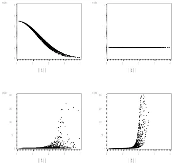
g2. . . 7 1.3 Importance sampling weights produced using four different importance
samplers (dimension=3). The top left plot results from an importance sampler with tails that decay more slowly than those of p∗(t) in all
directions. the top right plot results from an importance sampler that matches thep∗(t) exactly. The bottom left plot results from an
impor-tance sampler whose tails decay more quickly than those of the p∗(t)
in one dimension. The bottom right plot results from an importance sampler whose tails decay more slowly than those of the p∗(t) in all
three dimensions. See Section 1.3.1 for more details. . . 9 2.1 Comparison of the marginal density estimates of the EMVL (d=3)
pro-duced by fitting Laguerre polynomials (dashed line) and using Simp-son’s rule of integration (solid line). . . 30 2.2 Comparison of the marginal density estimates of the EMVL (d=5)
pro-duced by fitting Laguerre polynomials (dashed line) and using Simp-son’s rule of integration (solid line). . . 31 2.3 Comparison of the marginal density estimates of the EMVL (d=10)
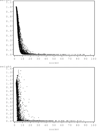
produced by fitting Laguerre polynomials (dashed line) and using Simp-son’s rule of integration (solid line). . . 31 2.4 Importance sampling weights using the posterior distributions from
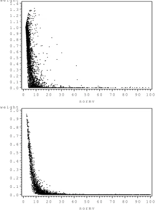
2.5 Importance sampling weights using the posterior distributions from Problems 3 (top figure) and 4 (bottom figure), untransformed Dirichlet and the EMVL as the importance sampler. The horizontal axes arekvk. 36 2.6 Importance sampling weights using the posterior distributions from
Problems 5 (top figure) and 6 (bottom figure), Untransformed Dirichlet and the EMVL as the importance sampler. The horizontal axes arekvk. 37 2.7 Importance sampling weights using the posterior distributions from
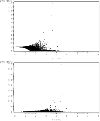
Problems 1 (top figure) and 2 (bottom figure), transformed Dirichlet and the EMVL as the importance sampler. The horizontal axes arekvk. 38 2.8 Importance sampling weights using the posterior distributions from
Problems 3 (top figure) and 4 (bottom figure), transformed Dirichlet and the EMVL as the importance sampler. The horizontal axes arekvk. 39 2.9 Importance sampling weights using the posterior distributions from
Problems 5 (top figure) and 6 (bottom figure), transformed Dirichlet and the EMVL as the importance sampler. The horizontal axes arekvk. 40 2.10 Importance sampling weights using the posterior distributions from
Problems 2 (top figure) and 6 (bottom figure), untransformed Dirichlet and the MVN as the importance sampler. The horizontal axes are kvk. 41 2.11 Importance sampling weights using the posterior distributions from
Problems 1 (top figure) and 5 (bottom figure), transformed Dirichlet and the MVN as the importance sampler. The horizontal axes are kvk. 42 2.12 90% confidence intervals and horizontal reference lines for the
equiv-alence interval (0.995, 1.005) is given. If the 90% confidence interval is completely contained within the equivalence interval, one concludes that the estimates are equivalent to 1 with 95% confidence. . . 45 3.1 Importance sampling weights resulting from four importance samplers
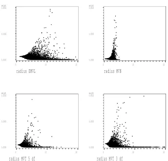
(EMVL, MVN, MVT with 5 degrees of freedom and 3 degrees of free-dom) used to estimate the normalization constant of the posterior dis-tribution in Example 1. The horizontal axes arekvk =kL−1(t−bt)k. A trend of weights that increase as kvk increases is an indication that the importance sampling estimates may not be asymptotically normal. 63 3.2 Importance sampling weights resulting from four importance samplers
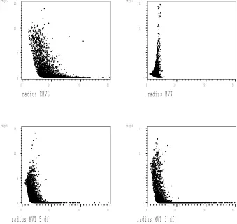
3.3 Importance sampling weights resulting from four importance samplers (EMVL, MVN, MVT with 5 degrees of freedom and 3 degrees of free-dom) used to estimate the normalization constant of the posterior dis-tribution in Example 3. The horizontal axes arekvk=kL−1(t−bt)k.A trend of weights that increase as kvk increases is an indication that the importance sampling estimates may not be asymptotically normal. 65 3.4 Importance sampling weights resulting from four importance samplers
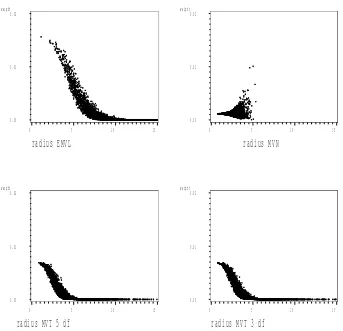
(EMVL, MVN, MVT with 5 degrees of freedom and 3 degrees of free-dom) used to estimate the normalization constant of the posterior dis-tribution in Example 4. The horizontal axes arekvk =kL−1(t−bt)k. A trend of weights that increase as kvk increases is an indication that the importance sampling estimates may not be asymptotically normal. 66 3.5 Importance sampling weights resulting from four importance samplers
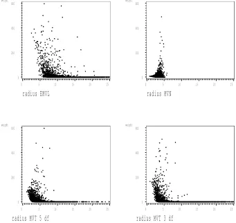
(EMVL, MVN, MVT with 5 degrees of freedom and 3 degrees of free-dom) used to estimate the normalization constant of the posterior dis-tribution in Example 5. The horizontal axes arekvk =kL−1(t−bt)k. A trend of weights that increase as kvk increases is an indication that the importance sampling estimates may not be asymptotically normal. 67 3.6 Importance sampling weights resulting from four importance samplers
(EMVL, MVN, MVT with 5 degrees of freedom and 3 degrees of free-dom) used to estimate the normalization constant of the posterior dis-tribution in Example 6. The horizontal axes arekvk =kL−1(t−bt)k. A trend of weights that increase as kvk increases is an indication that the importance sampling estimates may not be asymptotically normal. 68 3.7 Importance sampling weights resulting from four importance samplers
(EMVL, MVN, MVT with 5 degrees of freedom and 3 degrees of free-dom) used to estimate the normalization constant of the posterior dis-tribution in Example 7. The horizontal axes arekvk =kL−1(t−bt)k. A trend of weights that increase as kvk increases is an indication that the importance sampling estimates may not be asymptotically normal. 69 3.8 Importance sampling weights resulting from four importance samplers
(EMVL, MVN, MVT with 5 degrees of freedom and 3 degrees of free-dom) used to estimate the normalization constant of the posterior dis-tribution in Example 8. The horizontal axes arekvk =kL−1(t−bt)k. A trend of weights that increase as kvk increases is an indication that the importance sampling estimates may not be asymptotically normal. 70 3.9 Importance sampling weights resulting from four importance samplers
3.10 Importance sampling weights resulting from four importance samplers (EMVL, MVN, MVT with 5 degrees of freedom and 3 degrees of free-dom) used to estimate the normalization constant of the posterior dis-tribution in Example 10. The horizontal axes arekvk=kL−1(t−bt)k. A trend of weights that increase as kvk increases is an indication that the importance sampling estimates may not be asymptotically normal. 72 3.11 Hill Plots, as described in Section 3.2.2. The plots were produced using
the EMVL as the importance sampler. The top figure corresponds to Example 1, the bottom to Example 2. A horizontal reference line is drawn at the value of βb produced using k = 4n1/3 as suggested by Monahan (2001). . . 77 3.12 Hill Plots, as described in Section 3.2.2. The plots were produced using
the EMVL as the importance sampler. The top figure corresponds to Example 3, the bottom to Example 4. A horizontal reference line is drawn at the value of βb produced using k = 4n1/3 as suggested by Monahan (2001). . . 78 3.13 Hill Plots, as described in Section 3.2.2. The plots were produced using
the EMVL as the importance sampler. The top figure corresponds to Example 5, the bottom to Example 6. A horizontal reference line is drawn at the value of βb produced using k = 4n1/3 as suggested by Monahan (2001). . . 79 3.14 Hill Plots, as described in Section 3.2.2. The plots were produced using
the EMVL as the importance sampler. The top figure corresponds to Example 7, the bottom to Example 8. A horizontal reference line is drawn at the value of βb produced using k = 4n1/3 as suggested by Monahan (2001). . . 80 3.15 Hill Plots, as described in Section 3.2.2. The plots were produced using
the EMVL as the importance sampler. The top figure corresponds to Example 9, the bottom to Example 10. A horizontal reference line is drawn at the value of βb produced using k = 4n1/3 as suggested by Monahan (2001). . . 81 4.1 Estimates of β and coefficient of variation calculated for Example 1
using the EMVL as the importance sampler. The horizontal axes rep-resent the scale factor, cthat was used in matching the EMVL to the posterior distribution, p∗(t) by setting Σ−1, the inverse of the scaling matrix of the EMVL, equal to −c∇2lnp∗(t)|
t=ˆt. . . 90 4.2 Estimates of β and coefficient of variation calculated for Example 2
using the EMVL as the importance sampler. The horizontal axes rep-resent the scale factor, cthat was used in matching the EMVL to the posterior distribution, p∗(t) by setting Σ−1, the inverse of the scaling matrix of the EMVL, equal to −c∇2lnp∗(t)|
4.3 Estimates of β and coefficient of variation calculated for Example 3 using the EMVL as the importance sampler. The horizontal axes rep-resent the scale factor, cthat was used in matching the EMVL to the posterior distribution, p∗(t) by setting Σ−1, the inverse of the scaling matrix of the EMVL, equal to −c∇2lnp∗(t)|
t=ˆt. . . 92 4.4 Estimates of β and coefficient of variation calculated for Example 4
using the EMVL as the importance sampler. The horizontal axes rep-resent the scale factor, cthat was used in matching the EMVL to the posterior distribution, p∗(t) by setting Σ−1, the inverse of the scaling matrix of the EMVL, equal to −c∇2lnp∗(t)|
t=ˆt. . . 93 4.5 Estimates of β and coefficient of variation calculated for Example 5
using the EMVL as the importance sampler. The horizontal axes rep-resent the scale factor, cthat was used in matching the EMVL to the posterior distribution, p∗(t) by setting Σ−1, the inverse of the scaling matrix of the EMVL, equal to −c∇2lnp∗(t)|
t=ˆt. . . 94 4.6 Estimates of β and coefficient of variation calculated for Example 6
using the EMVL as the importance sampler. The horizontal axes rep-resent the scale factor, cthat was used in matching the EMVL to the posterior distribution, p∗(t) by setting Σ−1, the inverse of the scaling matrix of the EMVL, equal to −c∇2lnp∗(t)|
t=ˆt. . . 95 4.7 Estimates of β and coefficient of variation calculated for Example 7
using the EMVL as the importance sampler. The horizontal axes rep-resent the scale factor, cthat was used in matching the EMVL to the posterior distribution, p∗(t) by setting Σ−1, the inverse of the scaling matrix of the EMVL, equal to −c∇2lnp∗(t)|
t=ˆt. . . 96 4.8 Estimates of β and coefficient of variation calculated for Example 8
using the EMVL as the importance sampler. The horizontal axes rep-resent the scale factor, cthat was used in matching the EMVL to the posterior distribution, p∗(t) by setting Σ−1, the inverse of the scaling matrix of the EMVL, equal to −c∇2lnp∗(t)|
t=ˆt. . . 97 4.9 Estimates of β and coefficient of variation calculated for Example 9
using the EMVL as the importance sampler. The horizontal axes rep-resent the scale factor, cthat was used in matching the EMVL to the posterior distribution, p∗(t) by setting Σ−1, the inverse of the scaling matrix of the EMVL, equal to −c∇2lnp∗(t)|t=ˆt. . . 98 4.10 Estimates of β and coefficient of variation calculated for Example 10
using the EMVL as the importance sampler. The horizontal axes rep-resent the scale factor, cthat was used in matching the EMVL to the posterior distribution, p∗(t) by setting Σ−1, the inverse of the scaling matrix of the EMVL, equal to −c∇2lnp∗(t)|
4.11 Example 1: Comparison of importance sampling weights for conven-tional and alternate scale (c) when the EMVL was used as the im-portance sampler. The horizontal axes represent the radius, or kvk= kL−1(t−bt)k. . . 103 4.12 Example 2: Comparison of importance sampling weights for
conven-tional and alternate scale (c) when the EMVL was used as the im-portance sampler. The horizontal axes represent the radius, or kvk= kL−1(t−bt)k. . . 104 4.13 Example 3: Comparison of importance sampling weights for
conven-tional and alternate scale (c) when the EMVL was used as the im-portance sampler. The horizontal axes represent the radius, or kvk= kL−1(t−bt)k. . . 105 4.14 Example 4: Comparison of importance sampling weights for
conven-tional and alternate scale (c) when the EMVL was used as the im-portance sampler. The horizontal axes represent the radius, or kvk= kL−1(t−bt)k. . . 106 4.15 Example 5: Comparison of importance sampling weights for
conven-tional and alternate scale (c) when the EMVL was used as the im-portance sampler. The horizontal axes represent the radius, or kvk= kL−1(t−bt)k. . . 107 4.16 Example 6: Comparison of importance sampling weights for
conven-tional and alternate scale (c) when the EMVL was used as the im-portance sampler. The horizontal axes represent the radius, or kvk= kL−1(t−bt)k. . . 108 4.17 Example 7: Comparison of importance sampling weights for
conven-tional and alternate scale (c) when the EMVL was used as the im-portance sampler. The horizontal axes represent the radius, or kvk= kL−1(t−bt)k. . . 109 4.18 Example 8: Comparison of importance sampling weights for
conven-tional and alternate scale (c) when the EMVL was used as the im-portance sampler. The horizontal axes represent the radius, or kvk= kL−1(t−bt)k. . . 110 4.19 Example 9: Comparison of importance sampling weights for
conven-tional and alternate scale (c) when the EMVL was used as the im-portance sampler. The horizontal axes represent the radius, or kvk= kL−1(t−bt)k. . . 111 4.20 Example 10: Comparison of importance sampling weights for
4.21 Example 1: Comparison of importance sampling weights for conven-tional and alternate scale (c) when the MVN was used as the impor-tance sampler. The horizontal axes represent the radius, or kvk = kL−1(t−bt)k. . . 117 4.22 Example 2: Comparison of importance sampling weights for
conven-tional and alternate scale (c) when the MVN was used as the impor-tance sampler. The horizontal axes represent the radius, or kvk = kL−1(t−bt)k. . . 118 4.23 Example 3: Comparison of importance sampling weights for
conven-tional and alternate scale (c) when the MVN was used as the impor-tance sampler. The horizontal axes represent the radius, or kvk = kL−1(t−bt)k. . . 119 4.24 Example 4: Comparison of importance sampling weights for
conven-tional and alternate scale (c) when the MVN was used as the impor-tance sampler. The horizontal axes represent the radius, or kvk = kL−1(t−bt)k. . . 120 4.25 Example 5: Comparison of importance sampling weights for
conven-tional and alternate scale (c) when the MVN was used as the impor-tance sampler. The horizontal axes represent the radius, or kvk = kL−1(t−bt)k. . . 121 4.26 Example 6: Comparison of importance sampling weights for
conven-tional and alternate scale (c) when the MVN was used as the impor-tance sampler. The horizontal axes represent the radius, or kvk = kL−1(t−bt)k. . . 122 4.27 Example 7: Comparison of importance sampling weights for
conven-tional and alternate scale (c) when the MVN was used as the impor-tance sampler. The horizontal axes represent the radius, or kvk = kL−1(t−bt)k. . . 123 4.28 Example 8: Comparison of importance sampling weights for
conven-tional and alternate scale (c) when the MVN was used as the impor-tance sampler. The horizontal axes represent the radius, or kvk = kL−1(t−bt)k. . . 124 4.29 Example 9: Comparison of importance sampling weights for
conven-tional and alternate scale (c) when the MVN was used as the impor-tance sampler. The horizontal axes represent the radius, or kvk = kL−1(t−bt)k. . . 125 4.30 Example 10: Comparison of importance sampling weights for
4.31 Example 1: Comparison of importance sampling weights for conven-tional and alternate scale (c) when the MVT (5 degrees of freedom) was used as the importance sampler. The horizontal axes represent the radius, or kvk=kL−1(t−bt)k. . . 127 4.32 Example 3: Comparison of importance sampling weights for
conven-tional and alternate scale (c) when the MVT (5 degrees of freedom) was used as the importance sampler. The horizontal axes represent the radius, or kvk=kL−1(t−bt)k. . . 128 4.33 Example 4: Comparison of importance sampling weights for
conven-tional and alternate scale (c) when the MVT (5 degrees of freedom) was used as the importance sampler. The horizontal axes represent the radius, or kvk=kL−1(t−bt)k. . . 129 4.34 Example 5: Comparison of importance sampling weights for
conven-tional and alternate scale (c) when the MVT (5 degrees of freedom) was used as the importance sampler. The horizontal axes represent the radius, or kvk=kL−1(t−bt)k. . . 130 4.35 Example 1: Comparison of importance sampling weights for
conven-tional and alternate scale (c) when the MVT (3 degrees of freedom) was used as the importance sampler. The horizontal axes represent the radius, or kvk=kL−1(t−bt)k. . . 131 4.36 Example 3: Comparison of importance sampling weights for
conven-tional and alternate scale (c) when the MVT (3 degrees of freedom) was used as the importance sampler. The horizontal axes represent the radius, or kvk=kL−1(t−bt)k. . . 132 4.37 Example 4: Comparison of importance sampling weights for
conven-tional and alternate scale (c) when the MVT (3 degrees of freedom) was used as the importance sampler. The horizontal axes represent the radius, or kvk=kL−1(t−bt)k. . . 133 4.38 Example 5: Comparison of importance sampling weights for
List of Tables
2.1 Evaluation of Marginal Density Estimates for d= 1 . . . 27 2.2 Estimated Fourier Coefficients for dimensions 1, 3, 5 and 10 resulting
from fitting Laguerre polynomials to the marginal densities of the EMVL. 29 2.3 Dirichlet Distribution Parameters . . . 32 2.4 Entries are the t-statistics for testing the hypotheses H0 : E(Zi) = 1
and H1 :E(Zi)6= 1 . . . 44
2.5 Ratios of RM EV /qPni=1(Zi−Z·)2/n. . . 46
2.6 Lack of Coverage of 95% Confidence Intervals. Entries represent the proportion of times that a 95% confidence interval constructed using importance sampling estimates that failed to contain the true value of 1. 47 2.7 Results From Importance Sampling Using the EMVL . . . 48 3.1 Estimates of β for Examples 1-10 . . . 75 3.2 Relative standard errors of the importance sampling estimates of the
posterior distributions for Examples 1-10. Relative standard errors were not given when empirical evidence suggested that the importance sampling estimates were not asymptotically normal. . . 83 4.1 Resulting counts of the values of c chosen from 100 simulations for each
example, using the EMVL as the importance sampler. . . 89 4.2 Table ofβb, results of test of hypothesis of infinite variance, and relative
standard errors produced when an alternate scale was used to match the importance sampler, the EMVL, to the posterior distributions. For comparison, relative standard errors that resulted using the usual scale,c= 2 are also given. Relative standard errors were not reported if there was an indication that the importance sampling estimates were not asymptotically normal. . . 102 4.3 Hypothesis test for infinite variance of the importance sampling weights
4.4 Comparison of relative standard errors for Examples 1-10 . . . 116 4.5 Frequency of visits by length of stay for 132 long-term schizophrenic
patients (Wing, 1962) . . . 139 4.6 Importance Sampling Posterior Means and Corresponding Standard
Errors for Example 8 . . . 140 4.7 Importance Sampling Cell Count Estimates for Example 8. The
Chapter 1
Introduction
1.1
Motivation
In Bayesian statistics one often encounters the situation in which a random vector of interest, t ⊂ Θ, varies according to a unnormalized posterior distribution, p∗(t),
with a unique form whose properties are only known by its evaluation at abscissast. In this situation one frequently wishes to estimate some functional oft- most commonly
Ep∗[t] (the mean), andEp∗[tt0] (the covariance matrix). Other expectations that may
be of interest include the normalization constant of the posterior distribution and indicator functions. There are a number of techniques available to calculate
Ep∗{h(t)} =
R
h(t)p∗(t)dt
R
where h(t) is some function of t. One typically considers analytical solutions first. However, the number of posterior distributions for which one can integrate Equation 1.1 analytically is considerably few, especially in higher dimensions.
This leads to the consideration of numerical methods. Monte Carlo simulation is one of the most commonly used numerical methods for integration. In both small and large dimensions, Monte Carlo simulation is an option that permits integration over a broad range of posterior distributions. Random vectors, T(i), i = 1, .., n are generated from the distribution p∗(t). The average n−1Pn
i=1h(T(i)) is used to estimate Ep∗[h(t)]. This technique is feasible when it is easy to generate random
variables from p∗(t). However, in practice one rarely is able to generate from p∗(t),
and when it is possible, Ep∗[h(t)] usually is known (Monahan, 2000). An alternative
numerical method to consider is Monte Carlo Importance Sampling.
1.2
Monte Carlo Importance Sampling
This technique is similar to Monte Carlo integration, and can be used to integrate over unimodal, smooth posterior distributions. A sequence of n random variables, T(1),T(2), ...,T(n) is generated from some density, g(t), called the importance sam-pling density, or importance sampler. These generated values are used to calculate a weighted average of the h(T(i)). One can then estimate E
p∗[h(t)] by
hn=Eg{h(t)dw(t)}=n−1 n
X
i=1
where T(i) is the ith vector generated from g(t), and the function h(t) evaluated at
T(i) is given weight equal to w(T(i)). The weights are a ratio of the posterior and importance sampling densities, so that w(T(i)) = p∗(T(i))/g(T(i)).
The use of Equation 1.2 as an estimate of Ep∗[h(t)] follows from the fact that
Eg[h(t)w(t)] =
Z
h(t)[p∗(t)
g(t)]g(t)dt =
Z
h(t)p∗(t)dt
= Ep∗[h(t)],
where w(t) = p∗(t)/g(t).
1.3
Choosing an Importance Sampler
To be effective, an importance sampler should have certain properties. It should be relatively easy to generate random variables from g(t). In order to calculate the weights, one should be able to evaluate the density of g(t) up to a constant. In addition, one would like the density of g(t) to be similar to p∗(t).
It would also be useful to choose an importance sampler that results in importance sampling estimates that have a normal limiting distribution. It has been shown by Kloek and van Dijk (1987) and Geweke (1989) that hn converges almost surely to
Ep∗[h(t)] if:
2. {T(i) }∞
i=1 is a sequence of iid random vectors, the common distribution having a probability distribution g(t);
3. The support of g(t) includes Θ; and
4. Ep∗[h(t)] exists and is finite.
This is basically an application of the strong law of large numbers. Based on this result, one expects hn to be a good estimate of Ep∗[h(t)] for large values of n.
If, in addition to these assumptions, Eg[w(t)] and Eg[h(t)2w(t)] are finite then
(Geweke, 1989)
n12{h
n−Ep∗[h(t)]} ⇒N(0, σ2),
where
σ2 =
Z
{h(t)−Ep∗[h(t)]}2[p
∗(t)
g(t) ]g(t)dt.
One can estimateσ2 by
1
n
n
X
i=1
(h(T(i))w(T(i))−hn)2.
In practice it is often difficult, and sometimes impossible to verify that Eg[w(t)]
and Eg[h(t)2w(t)] are finite, especially when the dimension of the posterior
posterior distribution (Geweke, 1989). Since it is not necessary for the weights to be bounded (Monahan, 2001), one can attempt to verify empirically that an importance sampler decays more slowly than the posterior distribution for a sufficient distance in the tails. It should be noted that this type of verification cannot be taken as a proof that the importance sampling estimates are asymptotically normal, but rather as in-formal evidence that one should not reject the assumption of asymptotic normality of the importance sampling estimates.
If this condition is not satisfied, and the tails of the importance sampler decay more quickly than those of the posterior distribution, the tails of the posterior distributions will rarely be observed. The few values that are observed from the tails will dominate the sample because they will be given relatively large weights. In this situationhn is
still an unbiased estimator of Equation 1.1, but its variance may not be finite, so one cannot assume that the estimate of Ep∗[h(t)] is asymptotically normally distributed
(Geweke, 1989).
1.3.1
Illustrative Example
To see the effect of mismatching the tails of the posterior distribution, consider a one-dimensional example given by Monahan (2001). Let p∗(t) be the standard
distributions and the weightsp∗(t)/g1(t) and p∗(t)/g2(t). A reference line is drawn at
w(t) = p∗(t)/p∗(t) = 1. As can be seen in these figures, the first importance sampling
density,g1(t), has tails that are thicker thanp∗(t), and the resulting weights decrease as one moves away from the center of the distribution. In contrast, g2(t) has thinner tails than the posterior distribution, and the weights increase without bound as one moves away from the center.
A similar example can be given in three dimensions. Let p∗(t) be normally
dis-tributed with its mean at the origin, and covariance matrix
Σp∗ =
1 0 0 0 1 0 0 0 1
.
Consider four normally distributed importance samplers (g1(t), g2(t) and g3(t), and g4(t)) with means at the origin, and covariance matrices
Σg =
σ2
1 0 0 0 σ2
2 0 0 0 σ2 3 ,
where (σ2
P L O T p g 1 g 2 d e n s i t y
0 . 0 0 0 . 0 5 0 . 1 0 0 . 1 5 0 . 2 0 0 . 2 5 0 . 3 0 0 . 3 5 0 . 4 0 0 . 4 5 0 . 5 0
t
- 3 - 2 - 1 0 1 2 3
Figure 1.1: Posterior Density, p∗(t), and Importance Sampling Densities, g1(t) and
g2(t)
P L O T r e f e r e n c e w 1 w 2
w e i g h t
0 1 2 3 4 5 6 7 8 9 1 0 1 1
t
- 3 - 2 - 1 0 1 2 3
Figure 1.2: Corresponding Importance Sampling Weight Functions. A horizontal reference line is given at 1. The weights, w1, correspond to the weights produced using
the weights decrease askt|| increases. The importance sampler, g2(t), matches p∗(t)
perfectly. In this situation, as one might expect, all of the weights are one. This would rarely, if ever, happen in practice. The remaining two importance samplers show the problem that can arise when the tails of the importance sampler decay more quickly than those of the posterior distribution. The plot produced usingg3(t) demonstrates what can happen when the importance sampler decays more quickly than the posterior distribution in one dimension. The weights fan out and increase as ktk increases. The importance sampler g4(t) decays more quickly than the posterior distribution in all dimensions. Here the weights steadily increase as ktk increases.
Based on these examples, one might conclude thatg(t) should be chosen so that its tails decay as slowly as possible. However, when the tails of the importance sampler are much thicker than those of the posterior distribution, over sampling occurs in the tails of the posterior distribution. This results in miniscule weights being given to the observations from the tails of the posterior distribution. This can be a waste of computer time and can result in only a few observations contributing to the estimate of Ep∗[h(t)].
1.3.2
Common Importance Samplers
weight 0 1 2 3 4 5 ||t||
0 1 2 3 4
weight 0 1 2 3 4 5 ||t||
0 1 2 3 4
weight 0 50 100 150 200 ||t||
0 1 2 3 4
weight 0 50 100 150 200 ||t||
0 1 2 3 4
Figure 1.3: Importance sampling weights produced using four different importance samplers (dimension=3). The top left plot results from an importance sampler with tails that decay more slowly than those of p∗(t) in all directions. the top right plot
results from an importance sampler that matches thep∗(t) exactly. The bottom left
plot results from an importance sampler whose tails decay more quickly than those of the p∗(t) in one dimension. The bottom right plot results from an importance
sampler whose tails decay more slowly than those of thep∗(t) in all three dimensions.
−∇2lng
T(t)|t=ˆt, where bt is the posterior mode. This is based on large sample the-ory that the posterior distribution converges to the multivariate normal distribution (Geweke, 1989 and Monahan, 2001), and suggests that the multivariate normal dis-tribution would be a good choice for an importance sampling density. However, if the prior is improper, or flat for one of the parameters, the multivariate normal is not a good choice for an importance sampling density (Geweke, 1989). It should be noted that for most posterior distributions it takes relatively little computer time to calculate the posterior mode and Hessian, as opposed to calculating posterior means and variances which involve integrating over the posterior distribution.
Since it is preferable to use an importance sampler that has just slightly thicker tails than the posterior distribution, the best form for g(t) depends heavily on the form of the posterior distribution. Several distributions have been considered as importance samplers in the past. These include the Multivariate Normal distribu-tion, the Multivariate Student-t distribution with small degrees of freedom (Evans and Swartz, 1995, 2000), the Multivariate Split Normal and the Multivariate Split-t distribution (Geweke, 1989).
2000). The following sections in this chapter will briefly address how the Multivariate Normal distribution, the Multivariate Student-t distribution perform as importance samplers when the posterior distribution has tails that decay exponentially.
It should be noted that the Split Normal and Split Student t distributions are useful when the posterior density is substantially asymmetric (Geweke, 1989), but do not address the issue of exponentially decaying tails. The basic idea when using these distributions is to explore the posterior density along the axes in each direction and to find the slowest rate of decline. The importance sampling density (either the Multivariate Normal or Multivariate Student-t) is modified along each of these axes by this rate of decline. This does little to address the problem that arises when the posterior distribution has exponential tail behavior, since the tail rates of decay for the Split Normal and Split Student t distributions are the same as those of the Multivariate Normal and Multivariate Student-t respectively.
We propose using a generalization of the Multivariate Logistic Distribution as an importance sampler when it is suspected that the posterior distribution decays exponentially. Chapter 2 discusses some different generalizations of the Multivariate Logistic Distribution and their potential use as importance samplers.
behavior in the tails. When this happens any importance sampler may fail to per-form well (Geweke, 1989). We suggest modifying the manner in which the importance sampler is matched to the posterior distribution.
1.4
Multivariate Normal
The Multivariate Normal distribution (MVN) is one of the distributions most com-monly used as an importance sampler. To describe its form, letXbe ad-dimensional vector. Then X has a multivariate normal distribution (MVN) with mean µ and variance matrix Σ=LL0 if its probability density function is of the form:
fX(x) = 1
(2π)d/2|L|exp( 1
2(x−µ)
0Σ−1(x
−µ)),
whereLL0 is the Cholesky factorization ofΣ. To usefX(x) as an importance sampler
1.5
Multivariate Student-
t
The Multivariate Student-t (MVT) distribution is another distribution that is frequently used as an importance sampler. The d-dimensional vector, X has the MVT distribution with location parameter µ, scale parameter Σ, and k degrees of freedom if its probability density function is proportional to:
{1 + 1
d+k(x−µ)
0Σ−1(x
−µ)}−d+2k.
This distribution has been proposed as an alternative to the MVN for use as an importance sampler when the posterior density has heavier tails than the multivari-ate normal distribution. To use the MVT distribution as an importance sampler, it is matched to the posterior distribution at the mode by setting µ equal to the mode of the posterior, and Σ−1 equal to negative Hessian of the log of the posterior distribution.
Chapter 2
Characerizations of the
Multivariate Logistic Distribution
This chapter discusses four different generalizations of the Multivariate Logistic Distribution. Their potential use as importance samplers when the posterior distribu-tion of interest,p∗(t) has tails that decay at a rate similar to exp (−|t|) is investigated.
Three of the four generalizations have the form of the univariate logistic distribution when the one-dimensional case is considered. The univariate logistic distribution is described in Section 2.1. Each generalization g(t) was evaluated based on four criteria:
1. Generating random variables from g(t) should be relatively easy;
3. It should be possible to match g(t) to the posterior distribution at the mode;
4. The tails of g(t) should decay at an approximately exponential rate.
The first three criteria can be considered minimum qualifications for any impor-tance sampler. The final criterion is to determine if the proposed imporimpor-tance sampler would be useful when the posterior distribution has tails that decay at an exponen-tial rate. Only one of the four generalizations (the Elliptical Multivariate Logistic Distribution) proposed in this chapter meets all four requirements. This distribution is investigated first. Chapter 4 discusses the results of simulation experiments using the Elliptical Multivariate Logistic Distribution as an importance sampler. The three remaining generalizations fail to meet the minimum requirements for an importance sampler. These distributions are not investigated further.
2.1
Elliptical Multivariate Logistic
Distribution (EMVL)
This section discusses a generalization of the multivariate logistic distribution that meets all four of the criteria established at the beginning of this chapter. To define this distribution, let T be a d-dimensional random vector and kd a normalization
constant. The Elliptical Multivariate Logistic Distribution (EMVL) is defined as:
g(t) = (2π)−(d−21)·k
d· |L|−1
e−√(t−ˆt)0Σ−1(t−ˆt) (1 +e−√(t−ˆt)0Σ−1(t−ˆt)
where −∞< ti <∞, i= 1, . . , d and Σ=LL0.
When d= 1 the EMVL reduces to:
g(t) = σ−
1exp (−t/σ)
(1 + exp (−t/σ))2, − ∞< t <∞,
which is the form of the univariate logistic distribution with mean 0 and variance
σπ2/3. Clearly, the tails of the joint density (2.1) have an exponential rate of decline, so all that remains to be investigated are the other three requisites established at the beginning of this chapter. To further understand the properties of this distribution, the tail behavior of the marginal distributions will be investigated as well.
2.1.1
Generating from the EMVL
The first criterion established for a viable importance sampler was that it must be possible to generate random vectors from its distribution. A technique for generating random vectors from the EMVL makes use of the fact that the distribution of V = L−1(T−ˆt), where Σ =LL0, is spherically symmetric (i.e., the EMVL is elliptically
symmetric).
First note that the density of V can be written as:
gV(v) =cd·
e−√(v0v) (1 +e−√(v0v)
)2, − ∞< vi <∞,
where cd is a normalization constant. Now, consider a transformation of V, where
V=R·Z, R andZ are independent, and
R =kVk.
This transformation is discussed in some detail in Anderson (1984). It will be shown that it is possible to generate the random variable R and the random vector Z with relative ease, and hence possible to generate the random vector T.
The density function of the random variable R must be known in order to sample from its distribution. An expression for the density function can be found by noting that the density of V can be expressed as a function of V0V. This implies that the
density of R2 =V0V can be written as (Anderson, 1984):
fR2(r2) =
1
2Cd·m(r 2)
·(r2)12d−1
where Cd = 2π 1 2d
Γ(1 2d)
, the volume of a unit sphere in d dimensions, and
m(u) = c· e−
√
u2
(1 +e−√u2
)2, − ∞< u <∞.
A simple transformation of variables yields the distribution of R:
fR(r) = Cd·m(r)·rd−1
Random variables can be generated from this distribution using a ratio of uniform random variables (Kinderman and Monahan, 1977). This is done by generating two uniform random variables A and B, where the point (A,B) is uniformly distributed over the region
The ratio R=B/A has a density that is proportional to fR.
In practice this is done by noting that the region Cf often fits into a box with
vertices (0, b∗
+), (0, b∗−), (a∗, b∗+), (a∗, b∗−). One method of computing the vertices of
the box is to set:
a∗ = max
x {f
1/2(x) }
b∗+ = max
x {x·f
1/2(x) }
b∗− = min
x {x·f
1/2(x) }.
Then one simply uses the following acceptance-rejection algorithm to generate R (Monahan, 2001, pp 283-284):
1. Generate A ∼ Uniform (0, a∗)
2. Generate B ∼ Uniform (b∗
−, b∗+)
3. R=B/A
4. If A2 ≤f
R(R) then deliver R, else go to 1.
The second issue to address is the generation of the random vector Z. Since gV is a spherical distribution (i.e., gV is left invariant under the set ofd×d orthogonal matrices), Z is uniformly distributed over a d-dimensional unit sphere (Anderson, 1984). To verify that gV is a spherical distribution, consider Q, an orthogonal d×d matrix. Then,
gV(Qv) = c· |Q|
e−√v0Q0Qv
= c· e−
√
v0v (1 +e−√v0v)2 = m(v0v)
= gV(v).
Since Z is uniformly distributed over a unit sphere, one can generate Y where yi ∼
N(0,1); then Zi =Yi/kYk.
In conclusion, it is comparatively simple to generate random variables from this generalization of the Multivariate Logistic distribution since, to generateV, one sim-ply needs to generate R and Z. Then, since R and V are independent, V = R ·Z and T= ˆt+LV. Therefore, the EMVL satisfies the first requirement established at the beginning of this chapter.
2.1.2
Evaluating the Density Function
The second issue to address is the expression of the density function of the EMVL. The form for the density function is known and can be evaluated for a givent, except, perhaps, for the normalization constant,kd. The EMVL can be used as an importance
sampler for h(t) 6= 1, but in order to estimate the normalization constant of the posterior distribution, it is necessary to knowkd. An expression forkd, however, can
be found by noting that it is possible to write g(t) as a mixture of normals where S is a random variable with density qd(s) and
fT|S(t|s) = (2π)− d 2(1
s)
qd(s) = sd−1kd·dQ(s).
HeredQ(s) = dsdL(12s), and L is the Kolmogorov-Smirnov (K-S) distribution
L(s) = 1−2
∞
X
j=1
(−1)j−1exp(−2j2s2).
To show that
g(t) = Z
fT|S(t|s)qd(s)ds,
utilize the following result from Andrews and Mallows (1974) and Stefanski (1990). They demonstrate that the logistic distribution can be expressed as a Gaussian scale mixture:
f(t) = Z ∞
0 σ
−1φ(t/σ)dQ(σ)
= e−
t
(1 +e−t)2
where φ is the standard normal density. Using this fact,
g(t) =
Z (2π)−d 2
|L| (
1
s)
de−21s2(t−ˆt)0Σ−1(t−ˆt)k
d·sd−1dQ(s)
= (2π)− (d−1
2 )
|L|
Z 1
√ 2πe
−21s2(t−ˆt)0Σ−1(t−ˆt)k
d·s−1dQ(s)
= (2π)−(d−21)· kd
|L| ·
e−√(t−ˆt)0Σ−1(t−ˆt)
(1 +e−√(t−ˆt)0Σ−1(t−ˆt)
)2. Since R sd−1·k
ddQ(s) = 1, we see that kd = 1 for d=1, and kd is related to the
inverse of the (d−1)st moment of the K-S distribution for k >1. Using the form of
finds:
1
kd
= 2d−1E((1 2s)
d−1)
= 2(d−1)Γ( 1
2(d−1) + 1) 212(d−1)−1
∞
X
j=1
(−1)j−1j−(d−1)
= 212(d+1)Γ(1
2(d+ 1))
∞
X
j=1
(−1)j−1j−(d−1).
Since the value of kd can be computed using zeta functions (Abramowitz and
Stegun, 1974, Sec. 23), the criterion requiring that it be possible to evaluate the importance sampling density has been satisfied.
2.1.3
Matching the Posterior and the EMVL
The third requisite for an importance sampler is that it must be possible to match the importance sampler to the posterior distribution at the posterior mode. In other words, it must be possible to set ∇lng(t) |t=ˆt= 0 and −∇2lnp∗(t) |t=ˆt= −∇2lng(t)|
t=ˆt, where ˆt is the posterior mode. Again, definingv=L−1(t−ˆt), and noting that √v0v=qkvk2 one can write:
lng(t) = ln((2π)−(d−21)·k
d· |L|−1)−
q
kvk2−2 ln(1 +e−√kvk2
)
∇lng(t) = −Σ
−1(t
−ˆt) q
kvk2 + 2
e−√kvk2
1 +e−√kvk2
Σ−1(t−ˆt) q
kvk2 = −Σ−
1(t−ˆt) q
kvk2
(1−e−√kvk2
) (1 +e−√kvk2
)
.
Expandinge−√kvk2
for small kvk,
1−e−√kvk2
≈ qkvk2
and, since limt→ˆt(1 +e− √
kvk2
) = 2,
lim
t→ˆt∇lng(t) =
0 q
kvk2 · q
kvk2 2 = 0.
An expression for the Hessian of the EMVL evaluated at ˆtcan be found by writing:
∇2lng(t) = Σ−1(t−ˆt)(t−ˆt)0Σ−1 1−e
−√kvk2
(kvk2)3/2(1 +e−√kvk2
)− Σ−1 q
kvk2
1−e−√kvk2
1 +e−√kvk2
−Σ−1(t−ˆt)(t−ˆt)0Σ−1 2e
−√kvk2
kvk2(1 +e−√kvk2
)2
= Σ−1(t−ˆt)(t−ˆt)0Σ−11−e
−2√kvk2
−2qkvk2·e−√kvk2
(kvk2)3/2(1 +e−√kvk2
)2 − Σ−
1 q
kvk2
(1−e−√kvk2
) (1 +e−√kvk2
)
.
Expandinge−√kvk2
for small kvk,
1−e−2√kvk2
−2qkvk2·e−√kvk2
= 1−(1−2(qkvk2) + 4(kvk 2) 2! −8(kvk
2)3/2 3! +...)
−2qkvk2(1−qkvk2+kvk 2 2! −...) ≈ (kvk
2)3/2 3 and
1−e−√kvk2
Since limt→ˆt(1 +e−
√
kvk2
) = 2
lim
t→ˆt Σ
−1(t−ˆt)(t−tˆ)0Σ−1 1−e−2
√
kvk2
−2√kvk2·e−√kvk2
(kvk2)3/2 ·
1 (1+e−√kvk2
)2
= 0· 13 · 14
= 0
and
lim
t→ˆt
−Σ−1(1−e√kvk2
) q
kvk2(1 +e√kvk2
) = − ·Σ
−1
·qkvk2· 1 2qkvk2 = −1
2·Σ
−1
Therefore,
∇2lng(t)|t=ˆt=− 1 2Σ
−1,
and, to achieve proper scaling at the mode, set Σ−1 = −2∇2lnp∗(t) |
t=ˆt. Since it is possible to match the EMVL to the posterior distribution at the mode, the third requirement for an importance sampler has been met.
2.1.4
Tail Behavior of the Marginal Distributions of the EMVL
To further understand the properties of the EMVL, the marginal distributions of the EMVL, fTi(ti), i=1,...d, were examined. Obviously, when d= 1, the distribution
Even when one considers the case where d=2, the integral
fT2(t2) =
Z ∞
−∞c·
e−√t21+t22
(1 +e−√t21+t22)2
dt1
cannot be solved using basic calculus techniques. To address this problem two nu-merical methods were employed. For simplicity, consider the situation where ˆt = 0 and Σ=I.
The first method takes advantage of the characterization of the EMVL as a scale mixture of the MVN where the scale is related to the Kolmogorov-Smirnov distribu-tion (Secdistribu-tion 2.1.2). Since T|S is distributed as N(0,Is12) the marginal distribution
of Ti|S ∼N(0,s12). Using this fact and the distribution of S as Q, write
fTi(ti) =
Z ∞
0 1 √
2πs
d−2exp( −t
2
i
s2)dQ(s)
Again, save for d= 1, this integral cannot be evaluated easily using analytical meth-ods, but since the integration problem has now been reduced to one dimension, a nu-merical method can be used. Unfortunately, any nunu-merical method will only provide an approximation, no matter how good, of the true integral. However, these approx-imations can be examined for evidence of the behavior of the tails of the marginal distributions. One numerical method to consider is Simpson’s rule for integration. If
f is to be integrated over the interval [a,b], Simpson’s rule divides the interval into n
subintervals of the size h= (b−a)/n and estimates the integral as:
h[f(a) + 4
n
X
i=1
f(a+h2i−1
2 ) + 2
nX−1
i=1
It must be possible to evaluate the integrand at the endpoints of the subintervals in order to use Simpson’s rule. In this case, the value of dQ(s)is not easily evaluated for a given s, but since Q(s) can be evaluated with reasonable ease (Monahan,1989), it can be used to estimate dQ(s). This was done by fitting a natural cubic spline to Q(s) and using its derivative to estimate dQ(s). The domain of s was split into 30 subintervals over which a cubic function was fitted, forming the spline interpolant
d
Q(s) and its corresponding derivative qd(s). The estimate, fbTdi(ti) of the integral
b fti(ti) =
Z ∞
0 1 √
2πs
d−2exp( −t
2
i
s2)qd(s)ds was calculated using Simpson’s rule.
Just how good is the estimate of the marginal densities when the derivative of the spline is used to estimate dQ(s)? Since the value of the integralfTi(ti) is known when
d = 1, it is possible to calculate the difference between the estimate and the actual density. Simpson’s rule was used to calculate:
b I1 =
Z ∞
0 | b
fT1(t1)−fT1(t1)|dt1
b I2 =
sZ ∞
0 ( b
fT1(t1)−ft1(t1))2dt1
for k=5, 10, 15, 20, 25 and 30 subintervals (Table 2.1). The derivative of the spline estimate of Q(s) provides a good approximation of dQ(s) whend= 1 and a relatively large number of intervals is used.
intervals Ib1 Ib2 5 1.9577∗10−1 1.8584∗10−1 10 3.0959∗10−2 4.2805∗10−2 15 7.7655∗10−3 8.6364∗10−3 20 2.8487∗10−3 3.8848∗10−3 25 6.7694∗10−4 9.5239∗10−4 30 1.6685∗10−4 2.5576∗10−4
Table 2.1: Evaluation of Marginal Density Estimates ford= 1
not assume anything about the tail behavior of the marginal distributions. However, since the joint density decays at an exponential rate, if the assumption is made that the tails of the marginal density also decay exponentially, Laguerre polynomials can be used to approximate the marginal densities by expanding the marginal density,fTi,
in a Fourier series (Cencov, 1962 and Monahan, 2001): fTi(ti) =
P∞
j=0cjpj(ti), where
pj(t) = φj(t)·e−t. The φj(t), j = 0,1,2, .. are the series of complete orthonormal
functions as given in Monahan (2001):
φ0(t) = 1
φ1(t) = 1−t
φ2(t) = (2−4t−t2)/2
.
.
with recurrence formula: (n+ 1)φn+1(t) = (2n+ 1−t)φn(t)−nφn−1(t).
w(t) = et so that thep
j were orthogonal with respect to w(t). The marginal random
variables, Ti(l), l = 1, .., n were generated from a EMVL distribution. If the
assump-tion about the tail rate of decay was reasonable, the Fourier coefficients should become very small as j increases.
Forty-thousand random variables were generated from the EMVL distribution for each of d=1, 3, 5, and 10. A technical problem arose as the domain ofTi is (−∞,∞)
and the domain of the Laguerre polynomials is (0,∞). This problem was solved by noting that EMVL is symmetric about 0. The marginal densities then were estimated using the absolute value of the generated Ti values to fit the Fourier coefficients.
Then 2∗fTi(ti) was estimated by the Fourier series using the first k = 10 estimated
coefficients: fcTi(ti) =
Pk
j=0cˆjpj(ti). Table 2.2 shows the estimated coefficients up to
k = 15 for d= 1,3,5 and 10.
The fact that the Fourier coefficients become very small asjincreases provides fur-ther evidence in favor of the assumption that the marginal distributions have approxi-mately exponential tail behavior. As a further check, one can compare these marginal density estimates to those that were derived by fitting a spline. The marginal density estimates produced using Simpson’s rule for d=1, 3, 5, and 10 were calculated using 30 intervals to estimate the density at each ti. If our choice of Laguerre polynomials
ˆ
cj
j d=1 d=3 d=5 d=10
0 0.38554025 0.33821484 0.30710647 0.23282228 1 0.12935252 0.09083394 0.0742228 0.03436207 2 0.03011608 0.00848164 0.00648283 -0.00468211 3 -0.00361001 -0.01222448 -0.00755043 -0.00663721 4 -0.01189556 -0.01253462 -0.00713078 -0.00341662 5 -0.01142526 -0.0078907 -0.00450211 -0.00122777 6 -0.00863972 -0.00341648 -0.00259758 -0.00025016 7 -0.00574272 -0.00036605 -0.00159952 0.00013308 8 -0.00333541 0.00129475 -0.00114828 0.00030734 9 -0.00149763 0.00192163 -0.0009505 0.00041537 10 -0.00018355 0.00187115 -0.00086045 0.00048509 11 0.00066309 0.00142055 -0.00082753 0.00051319 12 0.00109363 0.00076615 -0.00083828 0.00049852 13 0.00116378 0.00004048 -0.00088221 0.00044822 14 0.00094103 -0.00067022 -0.00094021 0.00037392 15 0.00050452 -0.00131243 -0.00098585 0.00028690
d e n s i t y
- 0 . 0 20 . 0 0 0 . 0 2 0 . 0 4 0 . 0 6 0 . 0 8 0 . 1 0 0 . 1 2 0 . 1 4 0 . 1 6 0 . 1 8 0 . 2 0 0 . 2 2 0 . 2 4 0 . 2 6 0 . 2 8 0 . 3 0 0 . 3 2 0 . 3 4 0 . 3 6 0 . 3 8 0 . 4 0 0 . 4 2 0 . 4 4
t
0 1 2 3 4 5 6 7 8 9 1 0
Figure 2.1: Comparison of the marginal density estimates of the EMVL (d=3) pro-duced by fitting Laguerre polynomials (dashed line) and using Simpson’s rule of in-tegration (solid line).
very closely. Based on these empirical results, it is not unreasonable to conclude that the tails of the marginal distributions decay at a rate similar to exp (−|t|).
2.2
Simulation: Using the EMVL as an
Impor-tance Sampler for Dirichlet Posterior
Distri-butions
The EMVL passed all four requirements that were established at the beginning of the Chapter. As a further check, a simulation experiment was used to verify that using the EMVL as an importance sampler:
l 5
- 0 . 0 20 . 0 0 0 . 0 2 0 . 0 4 0 . 0 6 0 . 0 8 0 . 1 0 0 . 1 2 0 . 1 4 0 . 1 6 0 . 1 8 0 . 2 0 0 . 2 2 0 . 2 4 0 . 2 6 0 . 2 8 0 . 3 0 0 . 3 2 0 . 3 4 0 . 3 6
t
0 1 2 3 4 5 6 7 8 9 1 0
Figure 2.2: Comparison of the marginal density estimates of the EMVL (d=5) pro-duced by fitting Laguerre polynomials (dashed line) and using Simpson’s rule of in-tegration (solid line).
l 1 0
- 0 . 0 2 0 . 0 0 0 . 0 2 0 . 0 4 0 . 0 6 0 . 0 8 0 . 1 0 0 . 1 2 0 . 1 4 0 . 1 6 0 . 1 8 0 . 2 0 0 . 2 2 0 . 2 4 0 . 2 6
t
0 1 2 3 4 5 6 7 8 9 1 0
Problem dimension Parameters
1 3 21 22 23 24
2 3 3 4 5 6
3 3 5 10 15 20
4 7 21 22 23 24 25 26 27 28
5 7 3 4 5 6 7 8 9 10
6 7 3 4 5 10 16 21 22 23
Table 2.3: Dirichlet Distribution Parameters
2. produces standard errors of the estimates that are reasonable approximations of the true variability.
Twelve different normalized posterior distributions were considered. These posteriors were used by Monahan and Genz (1997) and consist of:
• six Dirichlet distributions with dimensions 3,3,3,7,7,7
• six transformed Dirichlet distributions with the same dimensions, transformed by 1+etet.
Table 2.3 gives the α parameters of the six densities from the Dirichlet family. The support of these densities is limited to the simplex Ptj ≤ 1, and the densities take
the form
Qd j=1t
αj−1
j (1−
P
tj)αd+1−1Γ(Pdj=1+1αj)
Qd+1
j=1Γ(αj)
The transformed Dirichlet densities use the change in variables
tj = e
xj
(1+Pdk=1exk), for j=1,....,d, with the resulting density over allR
d
ePdj=1αjxj
(1 +Pdj=1exj)
Pd+1 j=1αj
Γ(Pdj+1=1αj)
Qd+1
j=1Γ(αj)
.
A simulation experiment using 40,000 evaluations was done 100 times for each posterior distribution to estimate the integral R h(t)p∗(t)dt, where h(t) = 1. Since
the posterior distributions are normalized, the estimate of this integral should be one.
2.2.1
Evaluating the Weights
Before evaluating the estimates produced by the simulation study, it is important to determine that the requirements established in Chapter 1 appealing to the CLT have not been violated. One method of doing this is to examine the behavior of the weights, w(t), with respect to kvk, whereV =L−1(T−ˆt) and
w(t) = p∗(t)
g(t)
= p∗(t)
(2π)−(d−21) kd
|L−1| e
−√v0v
(1+e−√v0v
)2
.
If the weights decrease as kvk increases, it is reasonable to assume that the tails of the EMVL are thicker than those of the posterior distribution, and to proceed as though the importance sampling estimates are asymptotically normal.
any reason to question the assumption of asymptotic normality of the estimates of
Ep∗[h(t)].
w e i g h t
0 . 0 0 . 1 0 . 2 0 . 3 0 . 4 0 . 5 0 . 6 0 . 7 0 . 8 0 . 9 1 . 0 1 . 1
n o r m v
0 1 0 2 0 3 0 4 0 5 0 6 0 7 0 8 0 9 0 1 0 0
w e i g h t
0 . 0 0 . 1 0 . 2 0 . 3 0 . 4 0 . 5 0 . 6 0 . 7 0 . 8 0 . 9 1 . 0 1 . 1 1 . 2 1 . 3 1 . 4
n o r m v
0 1 0 2 0 3 0 4 0 5 0 6 0 7 0 8 0 9 0 1 0 0
w e i g h t
0 . 0 0 . 1 0 . 2 0 . 3 0 . 4 0 . 5 0 . 6 0 . 7 0 . 8 0 . 9 1 . 0 1 . 1 1 . 2 1 . 3 1 . 4
n o r m v
0 1 0 2 0 3 0 4 0 5 0 6 0 7 0 8 0 9 0 1 0 0
w e i g h t
0 . 0 0 . 1 0 . 2 0 . 3 0 . 4 0 . 5 0 . 6 0 . 7 0 . 8 0 . 9 1 . 0
n o r m v
0 1 0 2 0 3 0 4 0 5 0 6 0 7 0 8 0 9 0 1 0 0
w e i g h t
0 . 0 0 . 1 0 . 2 0 . 3 0 . 4 0 . 5 0 . 6 0 . 7 0 . 8 0 . 9 1 . 0 1 . 1 1 . 2
n o r m v
0 1 0 2 0 3 0 4 0 5 0 6 0 7 0 8 0 9 0 1 0 0
w e i g h t
0 . 0 0 . 1 0 . 2 0 . 3 0 . 4 0 . 5 0 . 6 0 . 7 0 . 8 0 . 9 1 . 0 1 . 1 1 . 2 1 . 3 1 . 4 1 . 5 1 . 6 1 . 7
n o r m v
0 2 0 4 0 6 0 8 0 1 0 0 1 2 0 1 4 0 1 6 0 1 8 0 2 0 0
w e i g h t
0 . 0 0 . 1 0 . 2 0 . 3 0 . 4 0 . 5 0 . 6 0 . 7 0 . 8 0 . 9 1 . 0 1 . 1
n o r m v
0 1 0 2 0 3 0 4 0 5 0 6 0 7 0 8 0 9 0 1 0 0
w e i g h t
0 . 0 0 . 1 0 . 2 0 . 3 0 . 4 0 . 5 0 . 6 0 . 7 0 . 8 0 . 9 1 . 0 1 . 1
n o r m v
0 1 0 2 0 3 0 4 0 5 0 6 0 7 0 8 0 9 0 1 0 0
w e i g h t
0 . 0 0 . 1 0 . 2 0 . 3 0 . 4 0 . 5 0 . 6 0 . 7 0 . 8 0 . 9 1 . 0 1 . 1
n o r m v
0 1 0 2 0 3 0 4 0 5 0 6 0 7 0 8 0 9 0 1 0 0
w e i g h t
0 . 0 0 . 1 0 . 2 0 . 3 0 . 4 0 . 5 0 . 6 0 . 7 0 . 8 0 . 9 1 . 0
n o r m v
0 1 0 2 0 3 0 4 0 5 0 6 0 7 0 8 0 9 0 1 0 0