Processes 2018, 6, x; doi: FOR PEER REVIEW www.mdpi.com/journal/processes
Article
1
Batch scheduling on a single machine with
2
maintenance interval
3
Honglin Zhang 1, Bin Qian 2 and Yaohua Wu 1*
4
1 School of Control Science and Engineering, Shandong University, Jinan 250061, China, [email protected]
5
2 Faculty of Information Engineering and Automation, Kunming University of Science and Engineering, Kunming 650500, China,
6
7
* Correspondence: [email protected]; Tel: +86 15666940680
8
Received: date; Accepted: date; Published: date
9 10
Abstract: In the manufacturing industry, orders are typically scheduled and
11
delivered through batches, and the probability of machine failure under high-load
12
operation is high. On this basis, we focus on a single machine batch scheduling
13
problem with a maintenance interval (SMBSP-MI). The studied problem is
14
expressed by three-field representation as 1|𝐵, 𝑀𝐼| ∑ 𝐹 + 𝜇 𝑚, and the optimization
15
objective is to minimize total flow time and delivery costs. Firstly, 1|𝐵, 𝑀𝐼| ∑ 𝐹 +
16
𝜇 𝑚 is proved to be NP-hard by Turing reduction. Secondly, shortest processing
17
time (SPT) order is shown the optimal scheduling of SMBSP-MI, and a dynamic
18
programming algorithm based on SPT (DPA-SPT) with the time complexity of
19
𝑂(𝑛 𝑇 ) is proposed. A small-scale example is designed to verify the feasibility of
20
DPA-SPT. Finally, DPA-SPT is approximated to a fully-polynomial dynamic
21
programming approximation algorithm based on SPT (FDPAA-SPT) by intervals
22
partitioning technique. The proposed FDPAA-SPT runs in 𝑂( ) time with the
23
approximation (1 + 𝜀).
24 25
Keywords: batch scheduling; single machine scheduling; maintenance interval;
26
dynamic programming; approximation algorithm
27 28
1. Introduction
29
Single machine scheduling problem is ubiquitous in manufacturing. As of
30
December 2019, the number of small and micro enterprises in China accounted for
31
82.5% of the national number [1]. Although modern manufacturing has shifted
32
toward intensification and large factories, in terms of quantity, small and micro
33
enterprises still make up a large proportion. Unlike large enterprises that have a
34
large number of machines and assembly lines, in small and micro enterprises,
35
especially micro enterprises, there is only one machine in the workshop production.
36
Due to the large number of machines in large enterprises, accidental machine failure
37
has little impact on the completion of the entire production plan. In 2017, a single
38
machine in the large-scale wafer factory of Magnesium Group failed, and the
39
maintenance of the machine took a lot of time, resulting in a serious lag in
40
production progress. The lag in production progress has led to insufficient capacity
41
of memory products using wafers as raw materials, which has triggered a surge in
42
the prices of related products worldwide. The influence of machine failure on large
43
enterprises is still the same. For small enterprises with only one or a few machines,
44
once one or several machines fail, it will be under a significant negative impact on
45
their production plans. It can be seen that despite the fact that the occurrence of
46
machine failure is a small probability event, once the machine fails, it will have many
47
adverse effects. By reasonably shutting down and inspecting the machine regularly,
48
the probability of machine failure can be greatly reduced.
49
In the actual production and trading process, the finished products are usually
50
delivered to customers in batches. Based on this fact, many scholars have conducted
51
research in the field of batch scheduling. Ikura etc. [2] studied single machine batch
52
scheduling problem with the goal of minimizing the maximum completion time. An
53
approximate algorithm was proposed, while the effect of this algorithm is not ideal.
54
Chang etc. [3] further studied the same problem and proposed a Simulated
55
Annealing Algorithm (SAA) with better optimization effect. In Chang’s paper,
56
Longest processing time (LPT) order was applied to optimize the initial solution of
57
SAA. Lee etc. [4] proposed a pseudo-polynomial time exact algorithm and a
58
complete polynomial time approximate algorithm to minimize total completion time
59
of SMBSP with dynamic job arrivals. Branch and bound algorithm (BBA) is another
60
algorithm that is commonly used to solve single machine batch scheduling problems.
61
For typical case, see reference [4]. In referrence [5], Azizoglu etc. proposed a BBA to
62
minimize total weighted completion time of SMBSP. In addition to the batch
single-63
machine scheduling problem, research on the single machine scheduling problem
64
with unavailable intervals (SMSP-UI) is also one of the research hotspots. Several
65
researchers have made progress in SMSP-UI. Sanlaville etc. [6] and Ma etc. [7]
66
independently reviewed the research in this field in recent decades. To optimize the
67
total weighted completion time of SMSP-UI, Ma etc. [8] proposed a dynamic
68
programming algorithm (DPA) and a BBA. both runs in pseudo-polynomial time.
69
Although both DPA and BBA are feasible, they are both pseudo-polynomial time
70
algorithms. In addition, Ma etc. [9] proposed a heuristic algorithm based on longest
71
processing time (LPT) order to minimize max completion time of SMSP-UI. Xie etc.
72
[10] designed a heuristic algorithm which runs in polynomial time to optimize
73
delivery time of SMSP-UI with job rejection. Luo etc. [11] studied a mew branch of
74
SMSP-UI, in which the maintenance time is related to workload. An approximate
75
algorithm running in polynomial time was proposed to optimize total weighted
76
completion time.
It is clear from the above literature review, however, despite the in-depth study
78
in the field of SMBSP and SMSPUI, single machine batch scheduling with
79
maintenance intervals (SMBSP-MI) is still a blind spot for research. Since the
80
outbreak of the COVID-19 virus in January 2020, the production capacity of major
81
mask manufacturers worldwide has been unable to meet demand, and a large
82
number of household mask factories have appeared in this context. Most of these
83
small mask factories work independently or independently from each other. Due to
84
the serious shortage of production capacity, mask machines usually need to work at
85
full load or overload, which greatly increases the probability of machine failure.
86
Therefore, it is necessary to carry out regular shutdown and maintenance of the
87
mask machine. This paper studies SMBSP-MI of a single mask machine scheduling
88
environment. First, the mathematical programming model of SMBSP-MI is
89
established, and then the SMBSP-MI is proved to be NP-hard. On this basis, shortest
90
processing time (SPT) order is proved the optimal scheduling rule of SMBSP-MI,
91
and a DPA based on SPT (DPA-SPT) is running in 𝑂(𝑛 𝑇 ) is proposed. Finally, an
92
approximate method is added to reduce the time complexity of DPA-SPT to
93
polynomial time.
94 95
2. Problem description
96
Since the outbreak of the COVID-19 virus in January 2020, the production
97
capacity of major mask manufacturers worldwide has been unable to meet demand,
98
and a large number of household mask factories have appeared in this context. Most
99
of these small mask factories work independently or independently from each other.
100
Due to the serious shortage of production capacity, mask machines usually need to
101
work at full load or overload, which greatly increases the probability of machine
102
failure. Therefore, it is necessary to carry out regular shutdown and maintenance of
103
the mask machine. This paper studies the maintenance scheduling problem in the
104
environment of a masking machine. The problem is described as follows: Mask
105
orders for multiple customers are processed on one mask machine. The factory
106
needs to process n quantities of raw materials into masks. Because different
107
customers have different delivery times, the raw materials are processed in batches.
108
Due to a large number of orders, the mask machine needs high-load work. To reduce
109
and avoid the probability of machine failure due to high-load work and ensure
110
smooth production, the factory regularly shuts down the mask machine for
111
maintenance. To ensure that the delivery schedule is not affected while overhauling,
112
the total process time and delivery cost of mask production are used as evaluation
113
indicators
114
The mathematical description of SMBSP-MI is: n jobs are processed in batches
115
on single machine. The set of jobs is 𝐽 = {𝑗 , 𝑗 , … , 𝑗 }. Jobs in J is divided into m
116
batches, i.e., 𝐵 = {𝐵 , 𝐵 , … 𝐵 , … , 𝐵 }, where 𝐵 represents a batch of jobs, and 𝐵
117
is the set of all batches. Once a batch of jobs is processed, it is delivered to the
118
customer. The unit batch delivery cost is 𝜇. A maintenance interval (MI) is set
during the machining process, where MI begins at time 𝑇 and ends at time 𝑇. No
120
job is allowed to be processed during MI. The goal is to optimize schedule of batches
121
and jobs, so that the sum of total flow time ∑ 𝐹 and delivery cost total 𝜇𝑚 is
122
minimized. SMBSP-MI is expressed by three-field representation as 1|𝐵, 𝑀𝐼| ∑ 𝐹 +
123
𝜇 𝑚.
124
The mathematical programming model of SMBSP-MI is expressed as follows.
125
min 𝑍 = ∑ 𝐹 + 𝜇𝑚 (1)
126
s.t.
127
∑ 𝐹 = ∑ 𝐹 (2)
128
𝐹 = 𝐹 + 𝐶 , 𝑖 > 1
𝐹 + 𝐶 , 𝑖 < 1 (3)
129
𝐶 = 𝐶 + 𝑝 + 𝛾(𝑇 − 𝑇 ), 𝑖 > 1
𝐶 + 𝑝 + 𝛾(𝑇 − 𝑇 ), 𝑖 < 1 (4)
130
𝛾 =
1 , 𝐶 + 𝑝 > 𝑇
0, 𝐶 + 𝑝 < 𝑇 , 𝑜𝑟 𝛾 =
1 , 𝐶 + 𝑝 > 𝑇
0, 𝐶 + 𝑝 < 𝑇 (5)
131
𝑝 ≤ 𝑇 < 𝑇 ≤ 𝜏 ∑ 𝑝 (6)
132 133
Formula 1 is the objective function, in which 𝐹 is flow time of the kth
134
scheduled batch, and 𝜇𝑚 is total delivery cost. Formula 2 indicates that the total
135
flow time of all jobs is equal to the sum of the flow time of all batches. This formula
136
makes it convenient to calculate the total flow time in an efficient way. Formula 3
137
indicates that the flow time of the ith job in the kth batch is equal to the sum of the
138
flow time of the previous processed job and the completion time of 𝐽 . i=1 means
139
that 𝐽 is the first job to be processed in the kth batch, thus the previous job of 𝐽 is
140
𝐽 i.e. the last job processed in the (k-1)th batch . The previous job of 𝐽 is 𝐽
141
while i >1, respectively. Formula 4 and 5 explains the calculation of 𝐽 ‘s completion
142
time, where 𝛾 is a 0-1 variable to judge whether 𝐽 is allowed to be processed
143
before MI. i.e. 𝐽 is allowed to be processed immediately while 𝐶 + 𝑝 < 𝑇 (or
144
𝐶 + 𝑝 < 𝑇 ), otherwise it is to be processed after MI. The strong constraint of
145
formula 6 ensures that the processing time of any job is not greater than 𝑇, and the
146
end of MI is not earlier than the sum of the processing time of all jobs.
3. The NP-hard attribute of SMBSP-MI
149
If 𝜇=0 and |MI| = 0, this problem is reduced to 1|𝐵| ∑ 𝐹, which is proved to be
150
NP-hard by Yang [12]. Obviously 1|𝐵, 𝑀𝐼| ∑ 𝐹 + 𝜇 𝑚 is more complicated than
151
1|𝐵| ∑ 𝐹 , hence is supposed to be an NP-hard problem. In what follows,
152
1|𝐵, 𝑀𝐼| ∑ 𝐹 + 𝜇 𝑚 is proved an NP-hard problem by reducing of equal-size
153
partition problem [13-15].
154
Equal-size partition problem is described as: Given a set 𝐼 =
155
(𝑎 , 𝑎 , . . . , 𝑎 , . . . , 𝑎 ), 𝑎 ∈ 𝑁∗, and ∑ 𝑎 = 2𝑀. Are there two disjoint subsets
156
𝐼 and 𝐼 , where |𝐼 | = |𝐼 | and ∑ ∈ 𝑎 =∑ ∈ 𝑎 = 𝑀?
157
Theorem 1. SMBSP-MI is an NP-hard problem.
158
Proof. The NP-hard attribute of SMBSP-MI is proved by the reduction of the
159
Equal-Size Partition Problem. Let 𝑀 ≥ 𝑢 + 2. The Equal-Size Partition Problem is
160
obviously meaningless when 𝑀 <𝑢 + 2, so the situation of 𝑀 <𝑢 + 2 is not considered.
161
An example of equal-size partition problem is established bellow, variables of
162
example see table 1.
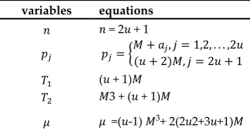
163 164
Table 1. variables of equal-size partition example
165
variables equations
𝑛 𝑛 = 2𝑢 + 1
𝑝 𝑝 = 𝑀 + 𝑎 , 𝑗 = 1,2, . . . ,2𝑢
(𝑢 + 2)𝑀, 𝑗 = 2𝑢 + 1
𝑇 (𝑢 + 1)𝑀
𝑇 𝑀3 + (𝑢 + 1)𝑀
𝜇 𝜇 =(𝑢-1) 𝑀3+ 2(2𝑢2+3𝑢+1)𝑀
U (Z threshold) 𝑈 =(3u-1)𝑀3 + 4(3u2+5u+2)𝑀
166
In what follows, we will prove that the equal-size partition problem has a
167
feasible solution, if and only if the constructed example has a solution which does
168
not exceed U. Let the sets 𝐼 and 𝐼 be the solutions to Equal-Size Partition
169
Problem. Let collection 𝐵 represent the set of jobs corresponding to set 𝐼 , 𝐴
170
represent the set of artifacts corresponding to collection 𝐼 .
171
Consider a situation where jobs in B are divided into one batch and processed
172
before 𝑇 , and jobs in A are divided into one batch and processed after 𝑇 . The
173
objective function is
𝑍 = ∑ 𝐹 + 2𝜇 = 𝑢 ∑ ∈ 𝑀 + 𝑎 + (+1) 𝑀 + (𝑢 + 1)𝑀 + ∑ ∈ { } 𝑀 +
175
𝑎 + (𝑢 + 2)𝑀 = 𝑢(𝑢 + 1)𝑀 + (𝑢 + 1)(𝑀 + 2(𝑢 + 1)𝑀 + (𝑢 + 2)𝑀) + 2 (𝑢 −
176
1)𝑀 + 2(2𝑢 + 3𝑢 + 1)𝑀 = (3𝑢 − 1)𝑀 + 4(3𝑢 + 5𝑢 + 2)𝑀
177
In this case the function value is exactly U.
178
Conversely, assume that there is a feasible schedule with the objective value not
179
exceeding U. Let B and A be the sets of jobs scheduled before 𝑇 and after 𝑇 ,
180
respectively. Then the following assertions hold:
181
1) The (2𝑢 + 1)th job is processed after 𝑇 ;
182
2) There are only two batches in this feasible schedule, one batch is processed before 𝑇
183
and another batch is processed after 𝑇 , respectively.
184
3) |𝐵| = 𝑢, |𝐴| = 𝑢 + 1;
185
4) ∑ ∈ 𝑝 = 𝑀.
186
The proof of these assertions is as follows:
187
1) The (2𝑢 + 1)th job is processed after 𝑇 because 𝑝 + 𝑀 > 𝑇;
188
2) Three possible cases are considered to prove assertion 2.
189
Case 1: There is one batch in this schedule, i.e. all jobs are processed after 𝑇 ,
190
and thus
191
∑ 𝐹 + 𝜇𝑚 = (2𝑢 + 1)𝑀(𝑀 + 3(𝑢 + 1)𝑀 + (𝑢 + 2)𝑀) + (𝑢 − 1)𝑀 +
192
2(2𝑢 + 3𝑢 + 1)𝑀 = 3𝑢𝑀 + (12𝑢 + 20𝑢 + 7)𝑀 > 𝑈 ,
193
which contradicts the constraint that 𝑍 = ∑ 𝐹 + 𝜇𝑚 ≤ 𝑈.
194
Case 2: Jobs are divided into more than two batches, i.e. there are at least two
195
jobs processed after 𝑇 .
196
∑ 𝐹 + 𝜇𝑚 > (2𝑢 + 1)𝑀(𝑀 + 3(𝑢 + 1)𝑀 + (𝑢 + 2)𝑀) + (𝑢 − 1)𝑀 +
197
2(2𝑢 + 3𝑢 + 1)𝑀 = 3𝑢𝑀 + (12𝑢 + 20𝑢 + 7)𝑀 > 𝑈 ,
198
which contradicts the constraint that 𝑍 = ∑ 𝐹 + 𝜇𝑚 ≤ 𝑈.
199
Case 3: Jobs are divided into two batches and both batches are processed after
200
𝑇 .
201
∑ 𝐹 + 2𝜇 − 𝑈 > (2𝑢 + 1)𝑀 + (𝑢 + 1)𝑀 − (𝑢 + 1)(𝑀 + 4(𝑢 + 1)𝑀) =
202
𝑀(𝑢𝑀 − 2𝑢 − 5𝑢 − 3) > 0 ,
203
which contradicts the constraint that 𝑍 = ∑ 𝐹 + 𝜇𝑚 ≤ 𝑈. The inequality
204
holds because 𝑀 ≥ 𝑢 + 2.
205
3) As shown in table 1, 𝑇 =(𝑢 + 1)𝑀 and 𝑝 > 𝑀, thus |𝐵| ≤ 𝑢. Take the case that |𝐴| ≥
206
𝑢 + 1 under consideration. Let ∑ ∈ 𝑝 = 𝐶 ≤ 𝑀 and |𝐴| = 𝑢 + 1 + 𝜗, 𝜗 ≥ 1.
∑ 𝐹 + 2𝜇 − 𝑈 = (𝑢 − 𝜗) (𝑢 − 𝜗)𝑀 + 𝐶 + (𝑢 + 1 + 𝜗)(𝑀 + (𝑢 + 1)𝑀 + (𝑢 +
208
𝜗)𝑀 + (2𝑀 − 𝐶) + (𝑢 + 2)𝑀) − ((𝑢 + 1)𝑀 + 4(𝑢 + 1) 𝑀) = 𝜗𝑀 + (2𝑢𝜗 +
209
2𝜗 + 6𝜗 + 1)𝑀 − (2𝜗 + 1)𝐶 ≥ 𝜗𝑀 + (2𝑢𝜗 + 2𝜗 + 6𝜗 + 1)𝑀 − (2𝜗 + 1)𝑀 >
210
0 ,
211
which contradicts the constraint that 𝑍 = ∑ 𝐹 + 𝜇𝑚 ≤ 𝑈. Thus |𝐴| ≤ 𝑢 + 1.
212
Considering the former assumption that |𝐴| ≥ 𝑢 + 1, we get |𝐴| = 𝑢 + 1, and
213
|𝐵| = 𝑢, respectively.
214
4) As shown in the proof of assertion 3, |𝐴| = 𝑢 + 1, |𝐵| = 𝑢. If 𝐶 < 𝑀, then
215 216
∑ 𝐹 + 2𝜇 − 𝑈 = 𝑢(𝑢𝑀 + 𝐶) + (𝑢 + 1)(𝑀 + (𝑢 + 1)𝑀 + 𝑢𝑀 + (2𝑀 − 𝐶) + (𝑢 +
217
2)𝑀) − ((𝑢 + 1)𝑀 + 4(𝑢 + 1) 𝑀) = (4𝑢 + 8𝑢 + 5)𝑀 − 𝐶 − 4(𝑢 + 1) 𝑀 = 𝑀 − 𝐶 >
218
0 ,
219
which contradicts the constraint that 𝑍 = ∑ 𝐹 + 𝜇𝑚 ≤ 𝑈. Thus 𝐶 ≥ 𝑀 .
220
Considering the former assumption that 𝐶 ≤ 𝑀, we get 𝐶 = 𝑀, and ∑ ∈ 𝑝 = 𝐶 =
221
𝑀.
222
The proof of proposed assertions is completed, Equal-Size Partition Problem has
223
a feasible solution. SMBSP-MI is NP-hard.
224
4. DPA-SPT
225
In this section, the Shortest Processing Time (SPT) order [16-19] is proved to be
226
the optimal scheduling rule of SMBSP-MI. And a Dynamic Programming Algorithm
227
(DPA) based on SPT is proposed after that.
228
Theorem 2. SPT order is the optimal scheduling rule of SMBSP-MI.
229
Proof. Assume that there is an optimal schedule that does not follow SPT order
230
𝑆 = (𝐵 , 𝐵 , . . . , 𝐵 , . . . , 𝐵 , . . . , 𝐵 , 𝑀𝐼, 𝐵 . . . , 𝐵 ),
231
in which 𝑝∈ > 𝑝∈ >. . . > 𝑝∈ >. . . > 𝑝∈ >. . . > 𝑝∈ > 𝑝∈ >. . . > 𝑝∈ . Take 𝑗 , i.e. the fth
232
job of the kth batch, and 𝑗 , i.e. the gth job of the lth batch with the inequality 𝑝 >
233
𝑝 . Exchange 𝑗 and 𝑗 , i.e. 𝑗 ∈ 𝐵 and 𝑗 ∈ 𝐵. A new schedule 𝑆 is established.
234
The objective Z with 𝑆 is increased by 𝑍 − 𝑍, comparing to it is with S.
235
𝑍 − 𝑍 = −(|𝐵 | + |𝐵 |+. . . +|𝐵 |)(𝑝 − 𝑝 ) > 0,
236
which contradicts the assumption that S is the optimal schedule of SMBSP-MI, and
237
thus 𝑝 ≤ 𝑝 . 𝑆 is the optimal schedule of SMBSP-MI, that is
238
S = (𝐵 , 𝐵 , . . . , 𝐵 , . . . , 𝐵 , . . . , 𝐵 , 𝑀𝐼, 𝐵 . . . , 𝐵 ),
in which 𝑝∈ ≤ 𝑝∈ ≤. . . ≤ 𝑝∈ ≤. . . ≤ 𝑝∈ ≤. . . ≤ 𝑝∈ ≤ 𝑝∈ ≤. . . ≤ 𝑝∈ .
240
Note that batches of schedule S are processed following SPT order, and sequence
241
of jobs in batch does not affect the flow time of this batch.
242
As is known, DPA is an exact algorithm, which implies that any step of DPA
243
meet the best choice. Since SPT is shown the optimal scheduling order of SMBSP-MI,
244
a DPA based on SPT order (DPA-SPT) is established as follows.
245
Since there are n jobs in total, DPA-SPT contains n cycles of iterations. Several
246
states are produced while containing the jth into S . Let 𝑅=(𝑠 , . . . , 𝑠 , . . . , 𝑠 ) be the
247
set of the states produced in the jth cycle of iteration, in which 𝑠 = (𝑙, 𝑐 , 𝑐 , 𝑎, 𝑡) is
248
one of the feasible states. Variables and parameters in 𝑠 are defined as follows: 𝑙
249
denotes finish time of the last job processed before 𝑇 ; 𝑐 denotes number of jobs
250
in the last batch processed before 𝑇 ; 𝑐 denotes number of jobs in the first batch
251
processed after 𝑇 (these jobs may be in the same batch with those processed before
252
𝑇 , if processing of the last batch is interrupt by MI); a denotes number of jobs
253
processed after 𝑇 ; t denotes the sum of current total flow time and delivery cost.
254
Since DPA select the optimal job in every cycle of iteration, the current optimal
255
schedule of SMBSP-MI before the jth iteration is 𝑆 = (1 , 2 , . . . , (𝑗 − 1) ).
256
And by comparing t values of all states produced in the following cycle of iteration,
257
the one with minimal t value is chosen as 𝑗 . And 𝑗 is at one of the possible
258
position on the machine, i.e. 𝑗 is located in the last batch processed before 𝑇 ;
259
𝑗 is located in one of other batches processed before 𝑇 ; 𝑗 is located in the
260
first batch processed after 𝑇 ; 𝑗 is located in one of other batches processed after
261
𝑇 , respectively. The optimal value 𝑍∗ will be found after all jobs are sequenced,
262
and the optimal schedule of SMBSP-MI will be decided by backtracking,
263
respectively.
264
The pseudo code of DPA-SPT is as follows.
265 266
Algorithm 1: DPA-SPT
Input: J, m, 𝜇, 𝑇 , 𝑇
Output: 𝑍∗
Initialization.
𝑅 = {(𝑝 , 1,0,0, 𝑝 + 𝜇), (0,0,1,1, 𝑇 + 𝑝 + 𝜇)};
Iteration.
For 𝑗 = 2 to n do
For (𝑙, 𝑐 , 𝑐 , 𝑎, 𝑡) ∈ 𝑅
If 𝑙 + 𝑝 ≤ 𝑇 and 𝑐 > 1 then
𝑠 = (𝑙 + 𝑝 , 𝑐 + 1, 𝑐 , 𝑎, 𝑡 + 𝑙 + (𝑐 + 1)𝑝 );
If 𝑙 + 𝑝 ≤ 𝑇 then
𝑠 = (𝑙 + 𝑝 , 1, 𝑐 , 𝑎, 𝑡 + 𝑙 + 𝑝 + 𝜇);
If 𝑐 > 1 then
𝑠 = (𝑙, 𝑐 , 𝑐 + 1, 𝑎 + 1, 𝑡 + 𝑇 + ∑ 𝑝 − 𝑙 + 𝑐 𝑝 );
Else then
𝑠 = (𝑙, 𝑐 , 1, 𝑎 + 1, 𝑡 + 𝑇 + ∑ 𝑝 − 𝑙 + 𝜇).
End if; End for;
For 𝑠 = (𝑙, 𝑐 , 𝑐 , 𝑎, 𝑡) ∈ 𝑅, 𝑠 = (𝑙, 𝑐 , 𝑐 , 𝑎 , 𝑡 ) ∈ 𝑅
If 𝑡 < 𝑡 then
Eliminate 𝑠 from 𝑅;
Else then
Eliminate 𝑠 from 𝑅 ;
End if; End for;
End for;
Optimization. 𝑍∗ = 𝑚𝑖𝑛( , , , , )∈ {𝑡}.
The optimal schedule is obtained by backtracking.
267
For any state 𝑠 = (𝑙, 𝑐 , 𝑐 , 𝑎, 𝑡), the upper bound of 𝑙 is 𝑇 , the upper bound of 𝑐
268
is n, the upper bound of 𝑐 is (n+1), and the upper bound of j is (n+1). Hence the
269
complexity of DPA-SPT is 𝑂(𝑛 𝑇 ), and thus DPA-SPT is a pseudo-polynomial time
270
exact algorithm.
271 272
To verify the feasibility of DPA-SPT, we present an illustrative 20-scale example.
273
The result shows that DPA-SPT achieves the optimal solution. In this sample,𝑚 = 4,
274
𝜇 = 500, 𝑇 = 90, 𝑇 = 120, and processing time of jobs are shown in table 2.
Table 2. Processing time of jobs
278
j 1 2 3 4 5 6 7 8 9 10 11 12 13 14 15 16 17 18 19 20
p 22 13 23 13 30 30 15 5 8 23 23 22 17 26 24 19 27 23 7 6
279
Sort jobs according to SPT order. The sorted schedule is shown in table 3.
280
Table 3. SPT schedule
281
j 8 20 19 9 2 4 7 13 16 1 12 3 10 11 18 15 14 17 5 6
p 5 6 7 8 13 13 15 17 19 22 22 23 23 23 23 24 26 27 30 30
282
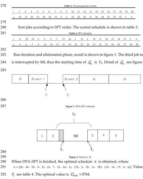
Run iteration and elimination phase, result is shown in figure 1. The third job in 𝐵
283
is interrupted by MI, thus the starting time of 𝑗 is 𝑇 . Detail of 𝑗 see figure 2.
284 285
B1 B2-part 1 B2-part 2 B3 B4
T1 T2
286
Figure 1. DPA-SPT schedule
287
1 2 MI 3 4 5
T1 T2
B2
288
Figure 2. Detail of 𝐵
289
When DPA-SPT is finished, the optimal schedule π is obtained, where
290
π = {(8,20,19,9,2),(4,7,13,16,1),(12,3,10,11,18),(15,14,17,5,6)}. Values of
291
𝐹 see table 4. The optimal value is 𝑍∗ =5784.
292 293
Table 4. Values of 𝐹
294
𝐹 𝐹 𝐹 𝐹 𝐹 𝐹 𝐹 𝐹 𝐹 𝐹 𝐹 𝐹 𝐹 𝐹 𝐹 𝐹 𝐹 𝐹 𝐹 𝐹 𝐹
5 11 18 26 39 52 77 137 156 178 200 223 246 269 292 316 342 369 399 429 3784
295
The example shows the feasibility of DPA-SPT.
296 297
5. FDPAA-SPT
Although DPA-SPT achieve best solution of small and medium scale problems,
299
it is not feasible for large-scale problems. With the expansion of the problem scale,
300
the complexity of DPA-SPT faces exponential dimension explosion. Taking into
301
account this problem, the use of elimination is the core of approximation to reduce
302
the complexity down to polynomial time. By pruning some bad states and the
303
application of state pruning technology[17], the solution space that the algorithm
304
needs to search is reduced, so as to reduce the complexity. In addition, due to
305
elimination operation, the optimal solution may be missed, hence the improved
306
algorithm is an approximate algorithm. In what follows, a fully-polynomial dynamic
307
programming approximation algorithm based on SPT (FDPAA-SPT) is designed.
308
Take two large number L and V, where 𝐿 ≤ 𝑍∗ ≤ 𝑉. Take a ε > 0, let 𝛿 = ,
309
𝛿 = . Divide [0, 𝑉] and [0, 𝑇 ] into and sub intervals, respectively. In
310
this way, [0, 𝑉] × [0, 𝑇 ] is divided into × subintervals.
311
To get a polynomial-time approximation schedule, the state set 𝑅 obtained by
312
the jth iteration of DPA-SPT is pruned. A new set 𝑅∗ is produced, and 𝑅∗ satisfies
313
the following attribute:
314
(1) 𝑅∗∈ 𝑅;
315
(2) There is only one 𝑅∗ in the same subinterval of × ;
316
(3) For any eliminated state (𝑙, 𝑐 , 𝑐 , 𝑎, 𝑡), there is a state (𝑙 , 𝑐 , 𝑐 , 𝑎 , 𝑡 ) ∈ 𝑅∗ locating in
317
the same subinterval with it.
318
The pseudo code of FDPAA-SPT is as follows.
319 320
Algorithm 2: FDPAA-SPT
Input: J, m, 𝜇, 𝑇 , 𝑇 , 𝐿, 𝑉, 𝛿 , 𝛿
Output: 𝑍∗
Initialization.
[0, 𝛿 ), [𝛿 , 2𝛿 ), … , 𝑽 − 1 𝛿 , 𝑉 ← [0, 𝑉];
[0, 𝛿 ), [𝛿 , 2𝛿 ), … , 𝑽 − 1 𝛿 , 𝑇 ← [0, 𝑇 ];
𝑅 = {(𝑝 , 1,0,0, 𝑝 + 𝜇), (0,0,1,1, 𝑇 + 𝑝 + 𝜇)};
Iteration.
For 𝑗 = 2 to n do
For (𝑙, 𝑐 , 𝑐 , 𝑎, 𝑡) ∈ 𝑅∗
If 𝑙 + 𝑝 ≤ 𝑇 and 𝑐 > 1 then
𝑠∗ = (𝑙 + 𝑝 , 𝑐 + 1, 𝑐 , 𝑎, 𝑡 + 𝑙 + (𝑐 + 1)𝑝 );
If 𝑙 + 𝑝 ≤ 𝑇 then
𝑠∗ = (𝑙 + 𝑝 , 1, 𝑐 , 𝑎, 𝑡 + 𝑙 + 𝑝 + 𝜇);
If 𝑐 > 1 then
𝑠∗ = (𝑙, 𝑐 , 𝑐 + 1, 𝑎 + 1, 𝑡 + 𝑇 + ∑ 𝑝 − 𝑙 + 𝑐 𝑝 );
Else then
𝑠∗ = (𝑙, 𝑐 , 1, 𝑎 + 1, 𝑡 + 𝑇 + ∑ 𝑝 − 𝑙 + 𝜇).
End if; End for;
For any 𝑠∗ = (𝑙, 𝑐 , 𝑐 , 𝑎, 𝑡) ∈ 𝑅∗
If 𝑙 > 𝑉 then
Eliminate 𝑠 from 𝑅∗;
Else
Keep 𝑠∗;
End for;
For 𝑠∗ = (𝑙, 𝑐 , 𝑐 , 𝑎, 𝑡) ∈ 𝑅∗, 𝑠∗ = (𝑙 , 𝑐 , 𝑐 , 𝑎 , 𝑡 ) ∈ 𝑅∗
If 𝑙 < 𝑙 and 𝑡 < 𝑡 then
Eliminate 𝑠∗ from 𝑅∗;
Else then
Eliminate 𝑠∗ from 𝑅∗;
End if; End for;
End for;
Optimization. 𝑍∗ = 𝑚𝑖𝑛( , , , , )∈ ∗{𝑡}.
The optimal schedule is obtained by backtracking.
The approximation process of FDPAA-SPT reduces its complexity to 1, and the gap
322
between the optimization solution and the approximate solution of FDPAA-SPT is
323
2. In what follows, the two conclusions are proved.
324
Theorem 3. For any eliminated state 𝑠 = (𝑙, 𝑐 , 𝑐 , 𝑎, 𝑡) ∈ 𝑅 , there exists a state
325
𝑠∗ = (𝑙 , 𝑐 , 𝑐 , 𝑎 , 𝑡 ) ∈ 𝑅∗, where 𝑙 < 𝑙 and 𝑡 < 𝑡 + 𝑛𝛿 + 𝑛𝑎𝛿.
326
Proof. Mathematical induction is used to prove theorem 3. When 𝑛 = 1, 𝑠 =
327
(𝑙, 𝑐 , 𝑐 , 𝑎, 𝑡) = 𝑠∗, theorem 3 holds. Assume that theorem 3 holds while 𝑛 = 𝑗 − 1,
328
i.e. for any eliminated state 𝑠 = (𝑙, 𝑐 , 𝑐 , 𝑎, 𝑡) ∈ 𝑅 , there exists a state 𝑠∗ =
329
(𝑙 , 𝑐 , 𝑐 , 𝑎 , 𝑡 ) ∈ 𝑅∗ , where 𝑙 < 𝑙 and 𝑡 < 𝑡 + (𝑗 − 1)𝛿 + (𝑗 − 1)𝑎𝛿 . When it
330
comes to 𝑛 = 𝑗, considering the diversity of states in 𝑅, 𝑠 may be produced from
331
one of the following former cases:
332
Case 1: 𝑠 = (𝑙 − 𝑝 , 𝑐 − 1, 𝑐 , 𝑎, 𝑡 − 𝑙 − 𝑐 𝑝 ) ∈ 𝑅 ;
333
Case 2: 𝑠 = (𝑙 − 𝑝 , 𝑥, 𝑐 , 𝑐 , 𝑡 − 𝑙 − 𝑝 − 𝜇) ∈ 𝑅 , 0 ≤ 𝑥 ≤ 𝑛 − 𝑐 − 1;
334
Case 3: 𝑠 = (𝑙, 𝑐 , 𝑐 − 1, 𝑎 − 1, 𝑡 + 𝑙 − ∑ 𝑝 − (𝑐 − 1)𝑝 ) ∈ 𝑅 ;
335
Case 4: 𝑠 = (𝑙, 𝑐 , 𝑦, 𝑎 − 1, 𝑡 − 𝑇 + 𝑙 − ∑ 𝑝 − 𝜇) ∈ 𝑅 ;
336
In what follows, we prove that no matter how 𝑠 is produced, it satisfies the
337
assumption of theorem 3.
338
In case 1, there is a state 𝑠∗ = (𝑙 , 𝑐 − 1, 𝑐 , 𝑎 , 𝑡 ) ∈ 𝑅∗ satisfying inequalities
339
𝑙 < 𝑙 − 𝑝 and 𝑡 < 𝑡 − 𝑙 − 𝑐 𝑝 + (𝑗 − 1)𝛿 + (𝑗 − 1)𝑎𝛿 . This judgment is clear due
340
to the assumption of 𝑛 = 𝑗 − 1. And in this case, inequality 𝑙 + 𝑝 ≤ 𝑙 ≤ 𝑇 holds.
341
By iteration phase of FDPAA-SPT, 𝑠 = (𝑙 + 𝑝 , 𝑐 , 𝑐 , 𝑎, 𝑡 + 𝑙 + 𝑎𝑐 ) ∈ 𝑅 is
342
produced, and inequalities 𝑙 < 𝑙 − 𝑝 and 𝑡 < 𝑡 − 𝑙 − 𝑐 𝑝 + (𝑗 − 1)𝛿 + (𝑗 −
343
1)𝑎𝛿 holds. According to elimination phase of FDPAA-SPT, there is a state 𝑠∗ =
344
(𝑙 , 1, 𝑐 , 𝑎 , 𝑡 ) ∈ 𝑅∗ locating in the same subinterval of 𝑅 with 𝑠. And 𝑙 ≤ 𝑙 +
𝑝 ≤ 𝑙 holds. Hence 𝑡 ≤ 𝑡 + 𝑙 + 𝑐 𝑝 + 𝛿 ≤ 𝑡 − 𝑙 − 𝑐 𝑝 + (𝑗 − 1)𝛿 + (𝑗 −
346
1)𝑎𝛿 + 𝑙 + 𝑐 𝑝 + 𝛿 < 𝑡 + 𝑗𝛿 + 𝑗𝑎𝛿 .
347
In case 2, there is state 𝑠∗ = (𝑙 , 𝑐 − 1, 𝑐 , 𝑎 , 𝑡 ) ∈ 𝑅∗ satisfying inequalities
348
𝑙 < 𝑙 − 𝑝 and 𝑡 < 𝑡 − 𝑙 − 𝑝 − 𝜇 + (𝑗 − 1)𝛿 + (𝑗 − 1)𝑎𝛿 . By iteration phase of
349
FDPAA-SPT, 𝑠 = (𝑙 + 𝑝 , 1, 𝑐 , 𝑎, 𝑡 + 𝑙 + 𝜇) ∈ 𝑅 is produced. According to
350
elimination phase of FDPAA-SPT, there is a state 𝑠∗ = (𝑙 , 1, 𝑐 , 𝑎 , 𝑡 ) ∈ 𝑅∗
351
locating in the same subinterval of 𝑅 with 𝑠 . And 𝑙 ≤ 𝑙 + 𝑝 ≤ 𝑙 holds. Hence
352
𝑡 ≤ 𝑡 + 𝑙 + 𝜇 + 𝛿 ≤ 𝑡 − 𝑙 − 𝜇 + (𝑗 − 1)𝛿 + (𝑗 − 1)𝑎𝛿 + 𝑙 + 𝜇 + 𝛿 < 𝑡 + 𝑗𝛿 +
353
𝑗𝑎𝛿 .
354
In case 3, there is state 𝑠∗ = (𝑙 , 𝑥, 𝑐 , 𝑎 , 𝑡 ) ∈ 𝑅∗ satisfying inequalities 𝑙 < 𝑙
355
and 𝑡 < 𝑡 + 𝑙 − ∑ 𝑝 − 𝑐 𝑝 + (𝑗 − 1)𝛿 + (𝑗 − 1)𝑎𝛿 . By iteration phase of
356
FDPAA-SPT, 𝑠 = (𝑙 , 𝑐 , 𝑐 , 𝑎 + 1, 𝑡 − 𝑙 + ∑ 𝑝 + (𝑐 − 𝑐 )𝑝 ) ∈ 𝑅 is produced.
357
According to elimination phase of FDPAA-SPT, there is a state 𝑠∗ =
358
(𝑙 , 1, 𝑐 , 𝑎 , 𝑡 ) ∈ 𝑅∗ locating in the same subinterval of 𝑅 with 𝑠. And 𝑙 ≤ 𝑙 ≤ 𝑙
359
holds. Hence 𝑡 ≤ 𝑡 − 𝑙 + ∑ 𝑝 + (𝑐 − 1)𝑝 + 𝛿 ≤ 𝑡 + 𝑙 − ∑ 𝑝 + (𝑐 −
360
1)𝑝 + (𝑗 − 1)𝛿 + (𝑗 − 1)𝑎𝛿 − 𝑙 + ∑ 𝑝 + (𝑐 − 1)𝑝 + 𝛿 = 𝑡 + (𝑙 − 𝑙 ) + 𝑗𝛿 +
361
(𝑗 − 1)(𝑎 − 1)𝛿 . Since 𝑙 ≥ 𝑙 − 𝑗𝛿 , 𝑡 ≤ 𝑡 + 𝑗𝛿 + 𝑗𝛿 + (𝑗 − 1)(𝑎 − 1)𝛿 < 𝑡 +
362
𝑗𝛿 + 𝑗𝑎𝛿 .
363
In case 4, there is state 𝑠∗ = (𝑙 , 𝑐 , 𝑦, 𝑎 , 𝑡 ) ∈ 𝑅∗ satisfying inequalities 𝑙 < 𝑙
364
and 𝑡 < 𝑡 − 𝑇 + 𝑙 − ∑ 𝑝 − 𝜇 + (𝑗 − 1)𝛿 + (𝑎 − 1)𝛿 . By iteration phase of
365
FDPAA-SPT, 𝑠 = (𝑙 , 𝑐 , 1, 𝑎 + 1, 𝑡 + 𝑇 − 𝑙 + ∑ 𝑝 + 𝜇) ∈ 𝑅 is produced.
366
According to elimination phase of FDPAA-SPT, there is a state 𝑠∗ =
367
(𝑙 , 𝑐 , 1, 𝑎 , 𝑡 ) ∈ 𝑅∗ locating in the same subinterval of 𝑅 with 𝑠 . Hence 𝑡 ≤
𝑡 + 𝑇 − 𝑙 + + ∑ 𝑝 + 𝜇 ≤ 𝑡 − 𝑇 + 𝑙 − ∑ 𝑝 − 𝜇 + (𝑗 − 1)𝛿 + (𝑗 − 1)𝑎𝛿 +
369
𝑇 − 𝑙 + ∑ 𝑝 + 𝜇 ≤ 𝑡 + 𝑗𝛿 + 𝑗𝑎𝛿 .
370
All the four cases meet theorem 3, thus theorem 3 holds. Hence there is a state
371
𝑠∗ = (𝑙 , 𝑐 , 𝑐 , 𝑎 , 𝑡 ) ∈ 𝑅∗ satisfying inequalities 𝑙 < 𝑙 and 𝑡 < 𝑡 + 𝑛𝛿 + 𝑛𝑎𝛿 =
372
𝑡 + 𝜀 + 𝜀 . Note that job n is processed after 𝑇 , thus 𝑡 > 𝑎𝑇 . Hence 𝑡 < 𝑡 + 𝜀 +
373
𝜀 = (1 + 𝜀)t. FDPAA-SPT get a (1 + 𝜀) approximate solution.
374
Theorem 4. The complexity of FDPAA-SPT is 𝑂( ).
375
Proof. In every iteration phase of FDPAA-SPT, × subintervals which
376
occupying space are produced. Since n is the maximum value of 𝑐 and 𝑐 ,
377
there are cases in every iteration of FDPAA-SPT. And after n cycle of iteration,
378
states are produced. Hence the complexity of FDPAA-SPT is 𝑂( ). It is very
379
clear that FDPAA-SPT runs in polynomial time.
380 381
6. Conclusion
382
In the manufacturing industry, orders are typically scheduled through batch
383
production and delivery mode, and the probability of machine failure under
high-384
load operation is high. On this basis, we focus on a single machine batch scheduling
385
problem with machine maintenance intervals. To solve this problem, the
386
mathematical programming model is established. SMBSP-MI is proved to be an
NP-387
hard problem, i.e., there is no exact algorithm that can obtain the optimal solution of
388
large-scale problems in polynomial time. Hence, we consider designing an
389
approximation algorithm that can obtain a high-precision solution in polynomial
390
time. Our approach is to design an accurate algorithm based on optimal rules in the
391
first place. Considering the dimensional explosion when solving large-scale
392
problems, some of the poor solutions obtained by DPA-SPT are eliminated to reduce
393
the complexity down to polynomial time. A small-scale example verifies the
394
feasibility of DPA-SPT. As for the proposed approximation algorithm, no
395
verification of the small and medium-scale is conducted, for the verification of the
396
small and medium-scale problem is meaningless. Besides, although the
397
approximation algorithm theoretically has a solution in polynomial time, it still
398
consumes a lot of calculation time, thus no large-scale calculation examples are
399
designed for verification. On the contrary, we proved that the approximate ratio of
400
the algorithm is (1 + 𝜀).
402
Author contributions: Investigation, Zhang, H. L.; Writing—original draft, Zhang,
403
H. L. and Qian, B.; Writing—review & editing, Zhang, H. L. and Wu, Y. H. All
404
authors have read and agreed to the published version of the manuscript.
405 406
Acknowledgments: The authors would like to thank Professor Yin Y. Q. (Doctoral
407
candidate, School of Management and Economics, University of Electronic Science
408
and Technology of China, China) for providing technical support, discussions and
409
review. First author would like to thank professor Qian, B., for providing guidance
410
at the beginning of the study and the initial review of abstract.
411 412
Conflicts of Interest: The authors declare no conflict of interest.
413 414
References
415 416
1. Xuan, T., Wei, Z., Weiwen, L., Huihong, L. Low-carbon sustainable development of China's
417
manufacturing industries based on development model change. Science of the Total
418
Environment,2020,737.
419
2. Ikura, Y., Gimple, M. Efficient scheduling algorithms for a single batch processing machine.
420
Operations Research Letters,1986, 5(2), 61-65.
421
3. Chang, P. Y., Damodaran, P., Melouk, S. Minimizing makespan on parallel batch processing
422
machines. International Journal of Production Research, 2004, 42(19), 4211-4220.
423
4. Lee, C. Y. Minimizing makespan on a single batch processing machine with dynamic job
424
arrivals. International Journal of Production Research, 1999, 37(1), 219-236.
425
5. Azizoglu, M., Webster, S. Scheduling a batch processing machine with non-identical job sizes.
426
International Journal of Production Research, 2000, 38(10), 2173-2184.
427
6. Sanlaville, E., Schmidt, G. Machine scheduling with avalibility constraints. Acta Information,
428
1998, (35):795-811.
429
7. Ma, Y., Chu, C., Zuo, C. A survey of scheduling with deterministic machine avalibility
430
constraints. Computers& Industrial Engineering, 2010, (58):199-211.
431
8. Ma, Y., Chu, C. B., Yang, S. L. Minimizing total weighted completion time in semiresumable
432
case of single-machine scheduling with an availability constraint. Systems Engineering-Theory
433
& Practice, 2009, 29(2), 134-143
434
9. Ma, Y., Yang, S. L., C. Cheng-Bin. Single machine scheduling with an availability constraint
435
and deteriorating jobs. Journal of Hefei University of Technology (Natural Science)
25.3(2007):778-436
781.
437
10. Xie, X., Xingyao, W., Xiaoli, L., Xiangyu, K. Production and transportation coordinated single
438
machine scheduling problems with unavailability interval and rejection. Journal of Shenyang
439
University (Natural Science). 2015, 27(3):222-225
440
11. Luo, W. C., Liu, F. On single-machine scheduling with workload-dependent maintenance
441
duration. Omega,2017,68:119-122.
442
12. Yu, Y., Tang, J. F., Li, J., Sun, W., Wang, J. W. Reducing carbon emission of pickup and
443
delivery using integrated scheduling. Transportation Research Part D 47, 2016, 237-250.
13. Corentin, L. H., Anne, L. L. Operations scheduling for waste minimization: a review. Journal
445
of Cleaner Production, 2019, 206, 211-226.
446
14. Yin, Y. Q., Cheng, T. C. E., Hsu, C. J., Wu, C. C. Single-machine batch delivery scheduling
447
with an assignable common due window. Omega, 2013, 41, 216-225.
448
15. Yin, Y. Q., Wang, Y., Cheng, T. C. E., Wang, D. J., Wu, C. C. Two-agent single-machine
449
scheduling to minimize the batch delivery cost. Computers & Industrial Engineering, 2016, 92,
450
16-30.
451
16. Qi, X., Bard, J. F., Yu, G. Disruption management for machine scheduling: the case of spt
452
schedules. International Journal of Production Economics, 103(1), 166-184.
453
17. Tang, G.C. Theory of modern scheduling. Shanghai science popularization press, 2003.
454
18. Brucker, P. Scheduling: Theory and Applications. Operations Research Proceedings 1997. 1998.
455
19. Pinedo, M. Scheduling: theory, algorithms, and systems. Tsinghua university press, 2005.
456
20. Yin, Y. Q., Cheng, T. C. E., Wang, D. J. Rescheduling on identical parallel machines with
457
machine disruptions to minimize total completion time. European Journal of Operational
458
Research, 2016, 252, 737-749.
459
© 2018 by the authors. Submitted for possible open access publication under the
460
terms and conditions of the Creative Commons Attribution (CC BY) license
461
(http://creativecommons.org/licenses/by/4.0/).