Emergence of shear bands in confined granular
systems: singularity of the
q-statistics
Léo Viallon-Galiner1, Gaël Combe1,∗, Vincent Richefeu1and Allbens Picardi Faria Atman2
1 Univ. Grenoble Alpes, CNRS, Grenoble-INP, Institute of Engineering Univ. Grenoble Alpes, 3SR, F-38000
Grenoble, France.
2 [Departamento de Física and National Institute of Science and Technology for Complex Systems,
CEFET-MG, Belo Horizonte, Brazil.
* Correspondence: [email protected]; Tel.: +33 4 56 52 86 29
Academic Editor: name
Version October 9, 2018 submitted to Preprints
Abstract: The statistics of grain displacements probability distribution function (pdf) during the
1
shear of a granular medium displays an unusual dependence with the shear increment upscaling
2
as recently evinced [Phys. Rev. Lett.115238301 2015]. Basically, thepdf of grain displacements has
3
clear nonextensive (q-Gaussian) features at small scales but approaches to Gaussian characteristics
4
at large shear window scales – thegranulenceeffect. Here, we extend this analysis studying a larger
5
system (more grains considered in the experimental setup) which exhibits a severe shear band fault
6
during the macroscopic straining. We calculate thepdf of grain displacements and the dependency
7
of theq-statistics with the shear increment. This analysis have shown a singular behavior ofqat
8
large scales, displaying a non-monotonic dependence with the shear increment. By means of an
9
independent image analysis, we demonstrate that this singular non-monotonicity could be associated
10
with the emergence of a shear band within the confined system. We show that the exact point where
11
theq-value inverts its tendency coincides with the emergence of a giant percolation cluster along the
12
system, caused by the shear band. We believe that this original approach using Statistical Mechanics
13
tools to identify shear bands can be a very useful piece to solve the complex puzzle of the rheology of
14
dense granular systems.
15
Keywords:Granular materials; Displacement fluctuations;q-Gaussian; strain localization
16
1. Introduction 17
The knowledge of the probability distribution function (pdf) for the velocities of systems composed
18
of particles is an essential information to assess the nature of microscopic interactions governing such
19
systems. A fundamental result of Statistical Mechanics concerns exactly the velocities pdf for a
20
collection of particles confined into a box, under the molecular chaos hypothesis, the celebrated
21
Maxwell-Boltzmann distribution [1]. Besides, under this assumption, collisions between particles
22
occur randomly, and it is thus possible to anticipate that the fluctuations in the particle velocities will
23
display apdf with Gaussian features. This is a consequence of the central limit theorem (clt), once the
24
particle velocity at a given timetis the result of a sequence of random events (collisions), leading to a
25
Gaussian distribution no matter how the events are themselves distributed.
26
These results are very robust and most of researchers take them asa priorifor data analysis.
27
However, in nature, several systems exhibit long range inter-particle interactions, a feature which
28
breaks one of the postulates of the molecular chaos hypothesis. In those systems, it is common to
29
observe important deviations from Gaussianpdf in the particle-fluctuation statistics. Tsallis and
30
collaborators [2] have shown that it is possible to extend thecltto consider systems which exhibit long
31
range or dissipative interactions by introducing theq-Gaussian distribution [3,4], where theqis an
32
additional parameter which allows to control the weight of thepdftail. In the limitq=1 the Gaussian
33
distribution is recovered, and forq6=1 heavy or light tails – platycurtic or leptokurtic distributions,
34
respectively – are obtained. Along the last years, Tsallis statistics were proven to successfully describe
35
several systems in high energy literature [5,6], magnetic systems [7,8], dissipative systems [9] and
36
remarkably several deviations from the Gaussian-like behavior were also reported in confined granular
37
systems [10–12].
38
Recently, studies with confined granular systems under shear introduced an additional problem
39
assessing the displacement fluctuationspdfof a given system (the displacement fluctuations correspond
40
to the displacement deviations from the mean field). The authors have demonstrated that thepdfsof
41
particle fluctuations are strongly dependent on the strain increment (akin to time scale) considered in
42
between the events [13,14]. Thepdfof fluctuations evolves from Gaussian-like, when large scales were
43
considered, to heavy tail distribution for small scales, which are well described byq-Gaussian up to five
44
decades for the magnitude of the fluctuations of displacements [15]. This unexpected result is indeed
45
quite robust as it was used to verify the Tsallis-Bukman scaling law [14,16] which relates theq-value
46
obtained from fluctuationpdf with the diffusion exponentα, related to the anomalous diffusion of
47
the grains [17]. Tsallis and Bukman have demonstrated that when long-range correlations are present
48
in the system, leading to an anomalous behavior in the path drift of particles, the corresponding
49
fluctuationpdf exhibits heavy tails, diverging from the Gaussian-like shape. The predicted relation
50
between these exponents, the Tsallis-Bukman scaling lawα=2/(3−q), was verified experimentally
51
by some works [11] but only at specific points. The first experimental verification of this law for a wide
52
range of points was made by Combe and collaborators for a confined granular system under shearing
53
[14]. It deserves to notice that the measures ofqandαwere completely independent, contributing to
54
the strength of this result.
55
Indeed, the shear experiment with heterogeneous granular media is an ideal system to study the
56
particle displacement fluctuations. It imposes a homogeneous deformation field over the system but,
57
due to the heterogeneous nature of the grains, the steric exclusion imposed by the rigidity of particles
58
implies a wide range of magnitude to the grain fluctuations along the experiment (see Supplementary
59
Material in [14]). Thus, a detailed evaluation of thepdf of grain fluctuations is essential to a proper
60
analysis of the microscopic interactions going on the system. In this work, we made a step further in
61
this direction by considering a system with a larger number of grains and shear rates at smaller inertial
62
numbers, but applying the same methodology as Combeet al.[14]. Not surprisingly, because of the
63
large number of particles, we have observed the development of shear bands during the experiments;
64
they are localized deformations which can span all along the system causing catastrophic effects.
65
After a careful image analysis, we have concluded that it is possible to associate the emergence of a
66
shear band with a sudden change in the value of theqparameter measured as a function of the time
67
scale. This singular behavior ofqassociated with a localization event in a confined granular system,
68
never reported before, opens a new perspective to use Statistical Mechanics tools as estimators for the
69
emergence of shear bands or even other analogous phenomena in granular systems and heterogeneous
70
media in general.
71
The paper is structured as follows: after this brief introduction we present the experimental
72
methodology and the details of the image analysis procedures. Next, we discuss the shear band
73
mechanics and our results under theq-statistic viewpoint. An image analysis of the particle fluctuations
74
considering percolation concepts is then discussed and compared with the preceding analysis. We
75
close the paper presenting our conclusions and some perspectives for future works.
76
2. Materials and Methods 77
2.1. Experimental setup
78
In this study, a 2D analogous granular material has been sheared with the 1γ2εshear apparatus [18,
79
19] at Laboratoire 3SR in Grenoble–France, Figure1. 1γ2εdevice is mainly a deformable parallelogram,
80
which deformation is controlled by five electric motors (two synchronized for height, two for width
81
and a last one for shear). Forces sensors installed at the corners of the parallelogram. They are used
to compute the stress applied to the granular material. Thanks to a retro-action loop, the size of the
83
parallelogram can be modified to impose a stress. All possible 2D strain and/or stress path can be
84
imposed to the granular media : uniaxial compression, isotopic compression, shear,etc. This apparatus
85
dedicated to granular materials have been used for research on various topics, such as the sensitivity
86
of the mechanical behavior to the stress loading path [19]; the influence of grain shape [20] with the
87
use of polygonal grains, mixed or not with round grains; the micro-mechanical investigations of the
88
effect of a highly deformable intruder in a confined granular media [21]; and the grain fluctuations in
89
a sheared granular assembly [14,22].
90
A
B
(a) (b)
Figure 1.(a) sketch of 1γ2εapparatus from [18]. (b) granular sample of 11 975Schneebelirods sheared in 1γ2ε. The inset is a zoom on a few rods of 5 different diameters, from 3.09 mm to 12.14 mm. Example of a segment[AB]used to assess theDICaccuracy.
The granular matter used in 1γ2εis a 2D analogous material called Schneebeli rods [23]. These
91
rollers of 6 cm long, named grains hereafter, are painted on their visible face with a speckle to be
92
followed during the test (see inset of the figure1b). For all experiments presented in this paper, the
93
granular samples were made of 11 975 grains with 5 different diameters sizes : 6 656 grains of 3.09 mm,
94
2 810 grains of 4.95 mm, 1 459 grains of 7.09 mm, 833 grains of 9.06 mm and 217 grains of 12.14 mm.
95
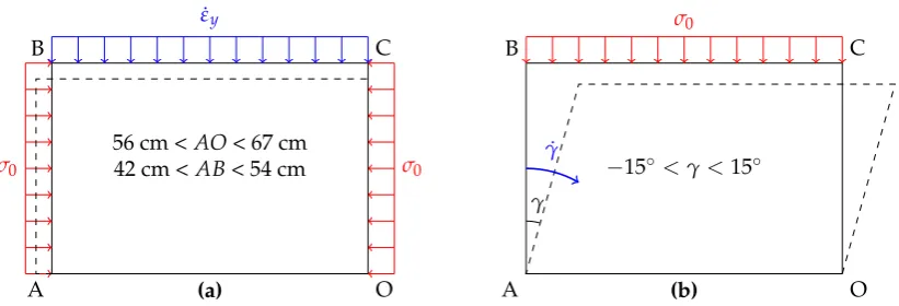
Two experimental tests were performed:
96
• vertical compression with an imposed vertical velocityv0(constant imposed vertical strain rate 97
˙
εy) with the lateral stress kept constant (σ0=50 kPa) – also calledbiaxial vertical compressionor 98
biaxial test;
99
• and shear test, for which 1γ2εparallelogram is tilted with an imposed shear rate ˙γ. During the
100
shear, the horizontal size of the sample is constant and a constant normal stressσ0in imposed on 101
the top of the sample. This test is also referred to assimple shear test.
102
The sketches of the principle of these tests are presented in Figure2. The imposed wall-velocity was
103
always sufficiently low to consider that the evolution of the granular assemblies is quasi-static,i.e.,
104
dynamic effect can be neglected. This could be ensured considering the dimensionlessinertial number
105
[24,25]I = γ˙d/√σ0ρ whereσ0is the confinement pressure,dis the mean grain diameter and ˙γis
106
the imposed shear rate. The largest inertial number used in this paper is about 10−6. It is now well
107
established that forI<10−3, dynamic effects can safely be ignored [25].
108
2.2. Assessment of the full grain-kinematics
109
Digital Image Correlation (DIC) is used to track each grain along all the photographs. This
110
technique was firstly suggested in [26] and largely developed since the beginning of the century to
111
provide kinematics fields from images (displacement, strain, accelerations,etc.) in continuous materials
(a) O A
B C
σ0 σ0
˙ εy
56 cm <AO< 67 cm 42 cm <AB< 54 cm
(b) O
A
B C
σ0
γ
˙ γ
−15◦<γ<15◦
Figure 2.Sketches of the two classical 2D tests realized: (a) a biaxial test and (b) a simple shear test. The imposed strain rates ( ˙εyor ˙γ) are displayed in blue, and the imposed stresses (σ0=50 kPa) are displayed in red. The straining ranges (extension lengths and tilting angles) permitted by the device 1γ2εare also provided.
(metals, polymers, concrete,etc.). In our case, the goal is not to determine strain fields fromlocal mean
113
displacements of an amount of grains but to follow the motion of each individual grain (supposed
114
to be rigid). The quantities to be determined are the displacement (components∆xand∆y) and the
115
rotation (∆θ) relative to the first image. This is very different from classical applications ofDICas
116
grains could move erratically and significantly between two successive images (especially in case of
117
grain rearrangements), so the variations∆x,∆y and∆θare not necessarily small or continuous in
118
space. Specific tools are thus needed to follow individual grains – without losing any of them and
119
with high precision of the tracked motions – in granular materials. The tool TRACKER[27] has been 120
developed exactly for this purpose.
121
The basis of theDICis to find the displacement of a pattern (subset of the reference image) on all
122
images. The best pixel position is chosen with the best correlation coefficientϕ, which is thezero-mean
123
normalized cross-correlation(ZNCC) coefficient. First, all positions and rotations are tested at pixels scale
124
in a ranged neighborhood of last known position of the grain by assuming that grains do not move a lot
125
during the 5 s between successive photographs; typically around 1 pixel. The recognition is supposed
126
to be correct ifϕis not under a given threshold (ϕ> 0.8), otherwise, the neighborhood ranges are
127
enlarged. At this point, the pixel position is given by integers and the rotation isquantizeddue to
128
the discrete nature of the signal. To refine the positions and rotations at a sub-pixel resolution, the
129
signal from second image is made continuous thanks to a bi-cubic interpolation of the gray levels, and
130
the best values of (∆x,∆y,∆θ) are found with a sub-pixel precision by minimizing(1−ϕ); Powell’s
131
conjugate direction method [28] is used to this end.
132
For Schneebeli rods, circular patterns centered on grains are used; their diameters are 80% of
133
the tracked grain diameters to avoid local deformations due to contact to be in the correlation area.
134
Localization of already identified grains are also used to reduce the search area and make the first
135
stage of the correlation faster. After the grain tracking, the positions are corrected to account for image
136
distortion with the Brown-Conrady model [29]. The scaling of images is done on the first images
137
with two points which distance is known at the beginning of the test. The movement of the camera is
138
corrected with the help of a set of points which are not supposed to move on the frame of the 1γ2ε
139
apparatus and covered by a speckle. Grains with an insufficient correlation coefficient (under 0.7) are
140
removed from the data by checking that they remain very few.
141
In all photographs, it is also possible to measure the mean stream, following the 4 corners of the
142
1γ2εwhich were also painted with a speckle. Finally, each grain comes with an actual motion and the
143
affine motion it would have if it obeys a homogeneous deformation gradient.
2.3. Accuracy of tracked kinematics
145
Accuracies of measurements of grain kinematics must take into account the full measurement
146
chain, from the camera lens to theDICsoftware. In particular, but not exclusively, inaccuracies come
147
from the lens distortion, the CCD sensor of the camera (that blur the image to avoid Moiré effects), the
148
algorithm used for demosaicing the image (Bayer matrix), the quality of the speckle painted on each
149
grain and the degree of complexity of the function of interpolation of the image (to obtain sub-pixel
150
measurements). A way to assess a reliable measurement of the error on the kinematics is to grab every
151
source of error together. Considering that the grains are perfectly rigid, any internal distance should
152
remain constant whatever the strain/stress path imposed to the granular sample,i.e., whatever the
153
displacements and the rotations of the grains. To test this, the two extremitiesAandBof several
154
segments are tracked together with the translation and rotation of all grains in the sample; see inset
155
in Figure1. Considering the first digital image as a reference, the initial lengthsL0i of the segmentsi
156
should not change for the other images. Therefore, the variations of length∆Li(N) = LNi −L0i as a
157
function of theNthimage provides an estimation of the kinematics error. The average errorsh∆L ii(N)
158
for each photograph were computed from 434 segments over more than 1 300 photographs that have
159
been shot during a shear test for which the maximum grain displacement was about 10 cm; Figure3.
160
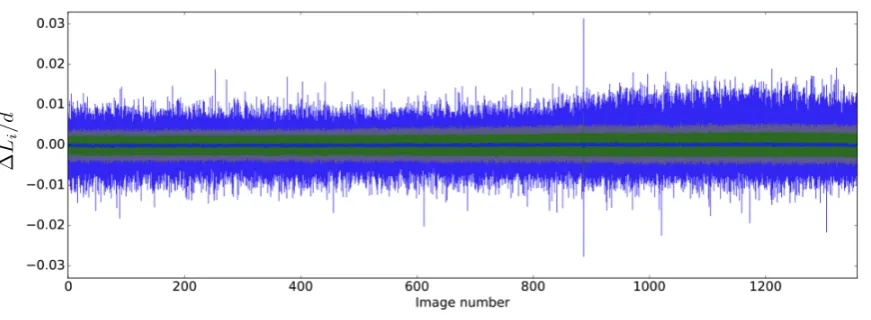
Figure 3.Segment length errors (relative to the mean diameter) over the photograph shots. Mean error h∆Lii/d(blue points close to zero), standard deviation (green area), 90thpercentile (gray area) and total range of errors (blue area) for all segments of each image since the first one (taken as reference). The set contained 434 segments.
In this example it is possible to observe a standard deviation of∆Liin the range±0.2% of the
161
mean-diameterdwith a nearly null average error. The distribution of errors∆Lifollows a Gaussian
162
function that remains nearly the same for all photographs. The maximum error is in the order of∼1%
163
of the mean diameter, and it goes exceptionally to∆Li/d=3% (this appended actually only one time
164
because of an unintentional kick in the camera). In view of the number of grains in each photograph,
165
this high level of accuracy was made possible thanks to a 80 MPixels digital Camera (PhaseOne iQ180
166
digital back) and a particular care to circumvent the possible sources of inaccuracy (correction of lens
167
distortion and camera parallax, check of pattern quality, choice of debayering algorithm, careful choice
168
of the interpolation function for sub-pixel gauging, uniform lighting,etc).
169
2.4. Fluctuation of the displacements
170
In a granular packing, a grain trajectory does not necessarily follow the homogeneous
171
displacement field imposed at the macroscopic level (sample scale). This is due to geometrical
172
constraints at the grain scale (steric exclusion) – grains are not able to displace as continuum mechanics
173
dictates they should. The fluctuation of displacement can be defined as the difference between the
actual displacementδr– measured withDIC– and the displacement that the same point would have if
175
it had obeyed a homogeneous strain (equals to the imposed macroscopic one)δr?.
176
It is useful to introduce a dimensionless fluctuationvas a ratio between the physical displacement fluctuation and the typical length∆εdwhere∆εis a homogeneous macroscopic strain anddis the
mean diameter of the grains:
v= δr−δr ?
∆εd (1)
Depending on the test,∆εcan be either an increment of shear strain (variation of the tilt angle)∆γ
177
or the vertical strain∆εy. The 1γ2εapparatus was designed so that the sample is disposed vertically,
178
that is to say the gravity acts on they component of our images which could introduce a bias in
179
the fluctuations. To avoid as much as possible this effect, it has been chosen to study mainly thex
180
coordinate of the fluctuations,vx.
181
2.5. Local strains
182
A local two dimensional strain tensor can be defined using the Delaunay triangulation of grain centers, where displacements are known. A mean strain tensor for each triangle is given thanks to the Stokes theorem as the contour integral:
ε= 1
S
Z
S∇u dS = 1
S
I
`u⊗n d
` (2)
whereuis the displacement vector at the boundary of the triangle, nthe outgoing normal vector,
183
S the triangle surface and ` the contour length, [19]. From the tensor ε, it is possible to use all
184
the components to highlight local/microscopic strains. But a convenient way to study the strain
185
localization in granular material is basically to focus on two invariants of the strain: the volumetric
186
strainεvol = trace(ε) = εI+εI I or the shear intensityεD = εI−εI I, whereεI ≥ εI I are the two
187
eigenvalues ofε. It should be noticed that the chosen sign convention is such that a strain component
188
is positive when lengths reduce. Figure4gives an example of a shear band network in a granular
189
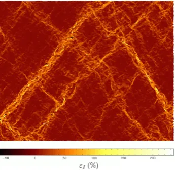
material subjected to a biaxial compression.
190
Hereafter, for a sake of simplicity, strain localization will generally be illustrated by means ofεD
191
which has the advantage of being always positive or equal to zero.
192
3. Shear band mechanism 193
When plasticity occurs in a heterogeneous material submitted to a deviatoric loading, strains can
194
concentrate in specific zones, and their locations are generally impossible to predict. These specific
195
zones are zones where the imposed strains on the sample (macroscopic scale) concentrates locally by
196
making patterns in the form of bands (see Figure4). These bands are termedshear bandssince they
197
are the places where the microscopic shear strain over-expresses, the rest of the volume being weakly
198
deformed compared with the mean strain. For dense granular material, it as been shown that strain
199
localization is a key mechanism of plasticity evolution. These shear bands are experimentally observed
200
either for sand [30], for analogous granular material likeSchneebelimaterials [19,31] and also for virtual
201
granular models like those used in DEM (Discrete Element Model) [32], or double scale FEM×DEM
202
(Finite Element Model at macroscopic scale, and Discrete Element Model at the microscopic scale) [33].
203
When a granular material is submitted to an external loading path, shear bands do not appear
204
instantaneously. During the past 50 years, many research works tried to explore and to understand
205
how shear bands appear and develop. Very recently, new progress inDICtechnique and with the
206
improvement of very high resolution of digital cameras helps to observe that shear banding can occurs
207
well before reaching the maximum strength of the granular assembly, [34]. But important questions
208
remain: why and how do the shear bands appear?
209
We focus here on the so-called vertical biaxial compression test. An imposed vertical strain
210
increases with a constant rate all along the compression. This strain rate is such that the sample
211
deforms in a quasi-static regime. At the end of the test, the macroscopic vertical strain can reach
212
εy=10 % or more. After a given macroscopic vertical strainεy(typically 2%), a network of oblique
213
shear bands can already be observed. Strain localized zones can be plotted and identified for a
214
given imposed macroscopic strain increment∆εyusing various local indicators like the increments
215
of the second invariant∆εD(shear intensity). Strain field of∆εDhave been computed for different
216
macroscopic strain increments∆εyfrom a macroscopic strain-level for which the shear bands have
217
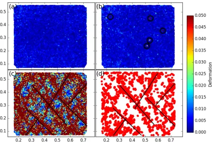
already started to develop,εy= 0.02. The first striking point is that when plotting the map of∆εD
218
for a very small increment∆εy=0.01%, the shear bands are not apparent, as shown in Figure5a. But
219
sometimes, for such very low strain increments, some concentrated local strain peaks occur, Figure5b.
220
It is possible to observed fully developed shear bands only for increments of strain greater or equal to
221
2%, as shown in Figure5c.
222
It is observed in Figure5c that the rare local peaks of∆εD, computed for the low strain increment
223
(∆εy=0.015%), reconstruct the picture of shear bands depicted in the Figure5d once aggregated in the
224
course of time. So, the concept of shear bands seem to be relevant only when a sufficient macroscopic
225
increment of strain is reached. This separates two regimes in term of∆εD: when the macroscopic
226
increment of strain is small, no extended localization zone appears except some very local microscopic
227
events with no manifest correlation in space; when the macroscopic strain reaches a sufficiently large
228
value, the imposed macroscopic strain localizes into shear bands that percolate throughout the granular
229
sample.
230
4. Shear bands: viewpoint ofq-statistics 231
4.1. q-Gaussian statistics of displacement fluctuations
232
When the strain is quite homogeneous throughout a deformed sample, thepdfof the normalized
233
displacement fluctuations follows aq-Gaussian. This was shown in [14] with a massive amount of
234
experimental data, but with systems with much less particles. A very clear broadening of the fluctuation
235
pdfswas observed as the strain increment∆εwas increased. Figure6a provides an illustration of such
236
broadening.
Figure 5.Vertical biaxial compression: field of local shear intensities∆εDfor different macroscopic strain increments∆εystarting from a state where shear bands are already established in the sample. (a) Field of local∆εDfor∆εy =0.015%; (b) Another case with∆εy=0.015% for which some Delaunay triangles present local peaks of∆εD(highlighted with circles); (c) shear intensity map for∆εy=2% showing shear bands in the material (highlighted by lines); (d) the localization of local strain peaks observed for increments∆εy=0.015%, aggregated over 2% of macroscopic strain; the lines are reported from the shear bands of (c).
10!
10!
10!
10!
10!
10
-40 -20 0 20 40
-1
-2
-3
-4
-5 0
1 1.1 1.2 1.3 1.4 1.5 1.6
0 10 20 30 40 q
1 1.1 1.2 1.3 1.4 1.5
0 20 40 60
q
(a) (b)
The dependence of theq-exponent with the strain increment∆εused to calculate the fluctuations
238
is shown in Figure6b, for experimental and numerical simulation data (the inset of the figure shows
239
the data issued fromDEMsimulations). Two remarkable features can be noticed with this plot:
240
• In the limit of large strain increments (i.ewhen the abscissa goes to zero)qtends to 1. In other
241
words, the distribution tends to become a Gaussian when∆ε → ∞. Some DEM simulations
242
made it possible to test larger values of∆ε, which confirm the limitq→1 (this data is shown in
243
the inset of Figure6b). This is exactly what is expected for this limit, once the particles typically
244
experience several contact losses/gains and rearrangements, approaching to the molecular chaos
245
hypothesis.
246
• At the other limit, for vanishing strain increment∆ε, theq-value attains a plateau that can be
247
interpreted as resulting from long range correlations imposed by the force chains at this short
248
displacement (or time) scale.
249
These features were observed both in experiments and also in a large number ofDEMsimulations,
250
which make the observations very robust provided that the assumption of strain homogeneity is not
251
too much jeopardized.
252
4.2. Evolution of q with emergence of shear bands
253
The fluctuations have been defined by assuming an affine field of displacements (or equivalently
254
a homogeneous field of strain) as expressed in Equation (1). However, as soon as strain localization has
255
a well-defined onset anywhere in the sample, the mean field of strains is not anymore a representative
256
quantity that reflects what actually happen. In spite of strain localization, the computation of
257
displacement fluctuations using Equation (1) remains possible, but its physical interpretation is
258
made more complex. Still, this measure is expected to continue to be of interest, as is the relying
259
q-statistical description.
260
The idea here is to study the evolution of theq-exponent when the strain increment is increased,
261
in the case of a clear localization of the strains through shear bands within the granular material. For
262
this purpose, a shear test was carried out (see the sketch of such loading in Figure2b). This loading
263
path was preferred because shear bands appear more progressively than with a biaxial compression,
264
so their studies are made easier. The evolution of theq-parameter regarding the (inversed squared)
265
increment of deformation is presented in Figure7.
266
When the macroscopic strain increment (here a shear strain increment∆γ) is sufficiently small,
267
the localization is not perceptible and similar observations than those of Section1can be drawn:
268
a transition from an invariant value ofqto a regime whereqstarts to go to 1 can be inferred for
269
1/√∆γ>12 (that is∆γ<0.7%). But when localization initiates (right vertical dashed line in Figure7),
270
an inflexion of the evolution ofqdrifts from the route towards 1. A third phase can be noticed when
271
∆γis even more increased for 1/√∆γ<7 (that is∆γ> 2%):qincreases suddenly which highlights a
272
new type of interactions in the grains displacements.
273
4.3. Link with the shear bands
274
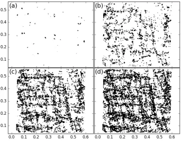
The shear bands can be visualized for different shear increments∆γin Figure8, where the shear
275
intensities∆εDhave been segmented thanks to a chosen threshold value∆ε0D: black zones correspond
276
to∆εD≥∆ε0Dand white zones correspond to∆εD <∆ε0D. The threshold value∆ε0Dhave been chosen
277
as the total macroscopic shear strain corresponding to the maximum achieved tilt, that is∆ε0D=3.6%,
278
and we checked that changing this value in the range 2.4% to 4.1% had no significant influence on the
279
observations presented below.
280
It can be noticed in these maps that, for lower strain increments (Figure8a), the bands are not
281
continuous at all, the highly sheared areas are very fragmented. For larger strain increments (Figures8b
282
and8c), these areas tend to aggregate in the form of bands, and on Figure8d, the bands seem to be
1 1.05 1.1 1.15 1.2 1.25 1.3
0 10 20 30 40 500
20 40 60 80 100 120
(a)
(b)
(c) (d)
q `/d
1/√∆γ
q 1 + 0.28 tanh(0.095/√∆γ) `/d
Figure 7.Evolution of theq-exponent of thepdfsof displacement fluctuations, and of the maximal length of shear bands`/d(number of mean diameters), when the shear strain increment∆γis increased (from right to left). The gray dashed line serves as guide to the eyes; the “tanh” function has no particular meaning excepted that it tends to 1 when∆γ→∞and it saturates at a plateau-value when∆γ→0. The vertical dashed lines indicate two transitions of both curves (qand`/d): from right to left, the first transition corresponds to the point whereqstarts to derive from the route to 1 (“tanh” function) and`/dstarts to take off; the second transition corresponds to the surge of bothqcorrelated with the percolation of the shear band throughout the sample.
Figure 8.Shear intensity map segmented with a threshold∆ε0
continuous from one border of the sample to an other. These four maps are spotted in Figure7so that
284
the relationship with theq-values can be done.
285
To better relate the growth of shear bands with theq-parameters, a new indicator is introduced:
286
the maximal length`of the shear bands. For each contiguous area of high shear strain (in black),
287
the length`is defined as the longest distance joining two grain centers belonging to the same area,
288
using the infinite norm (that is the maximal amplitude overxory). The indicator is then the largest
289
length for all contiguous area of high shear strain on the map. The evolution of this maximal length,
290
expressed in number of mean diameters`/d, is plotted as a function of 1/√∆γin Figure7in order to
291
draw a parallel with the evolution ofq. For smallest strain increments (right of abscissa)`is of the
292
order of a few diameters, which indicates that a few grains are involved and thus these “shear bands”
293
are actually local rearrangements. A faster evolution of`can then be noticed with an inflexion point
294
corresponding nearly at the start ofqdrift. Finally, unlike what the maps in Figure8may suggest,
295
the evolution of the length of the shear bands is not steady. A clear transition arises with length of
296
shear bands reaching suddenly the sample size. This transition occurs precisely for the same strain
297
increment that the transition observed with theq-parameter in Figure7. This latter observation is not
298
sensitive to threshold value employed in the analysis, which makes it very robust.
299
So, the raise of theq-parameter for largest increments of deformation could be assigned to the
300
percolation of shear bands, as it occurs exactly when the shear bands extension reach the sample size.
301
Besides, we found a linear dependence betweenqand` as the shear band length grows (data not
302
shown), with a negative linear coefficient up to the percolation transition. This is an strong evidence
303
that these two parameters are (anti-)correlated and, thus, both can be used as order parameter for the
304
transition. The possibility to anticipate the shear band formation by means of a direct measure over
305
the system is a very sound tool, and here we report very promising results in this direction.
306
5. Conclusions 307
The nature of grain displacement fluctuations in confined granular systems under shear was
308
investigated by means of statistical mechanics tools. We extend previous work which demonstrated
309
an unusual dependence of the nonextensive parameter q with the shear strain window scale by
310
characterizing the emergence of a shear band along the system. Our results have shown that the
311
q-parameter displays a singular non-monotonic behavior at large scales. Performing an independent
312
image analysis, we identify the emergence of a giant percolation cluster in the system associated with
313
the shear band localization. By comparing the behavior of the percolation order parameter and the
314
q-parameter dependence with the shear strain window scales has evinced a remarkable correlation
315
between the emergence of the shear band along the system and the sudden change in theq-value. This
316
remarkable observation obtained by an original approach with non-extensive statistical mechanics
317
tool has a great potential to impact the research field and also to other areas which deals with similar
318
systems.
319
We expect to perform more analysis concerning the character of the displacement fluctuations
320
inside the shear bands themselves (like in [35]). It is also planed to explore larger systems (with more
321
grains) and slower loadings (lower inertial numbers) in future investigations. We believe that the
322
approach introduced here has the potential to reveal interesting findings and new perspectives in
323
regard of the very special character of grain kinematics in confined granular systems.
324
Author Contributions:L V-G and G C performed the experiments. L V-G, G C, V R and APF A wrote the paper. 325
Funding:APF A thanks to brazilian agencies FAPEMIG and CNPq by financial support. The Laboratoire 3SR is 326
part of the LabEx Tec 21 (Investissements d’Avenir - grant agreement noANR-11-LABX-0030) 327
Acknowledgments:We are in debt to Constantino Tsallis for the fruitful discussions and suggestions. APF A and 328
G C thanks to 3SR Laboratory and ComUE Université Grenoble Alpes for the funding APF A visit in 2017. 329
Abbreviations 331
The following abbreviations are used in this manuscript: 332
333
pdf Probability Density Function clt central limit theorem DIC Digital Image Correlation DEM Discrete Element Model FEM Finite Element Model 334
335
1. Tolman, R.The principles of statistical mechanics; Dover Publications: New York, 1979. 336
2. Umarov, S.; Tsallis, C.; Steinberg, S. On a q-Central Limit Theorem Consistent with Nonextensive Statistical 337
Mechanics. Milan Journal of Mathematics2008,76, 307–328. doi:10.1007/s00032-008-0087-y. 338
3. Tsallis, C. Possible generalization of Boltzmann-Gibbs statistics. Journal of statistical physics1988, 339
52, 479–487. 340
4. Tsallis, C.Introduction to nonextensive statistical mechanics: approaching a complex world; Springer Science & 341
Business Media, 2009. 342
5. Marques, L.; Andrade-II, E.; Deppman, A. Nonextensivity of hadronic systems. Phys. Rev. D2013, 343
87, 114022. doi:10.1103/PhysRevD.87.114022. 344
6. Wilk, G.; Włodarczyk, Z. The imprints of nonextensive statistical mechanics in high-energy collisions. 345
Chaos, Solitons & Fractals2002,13, 581 – 594. Classical and Quantum Complexity and Non-Extensive 346
Thermodynamics, doi:https://doi.org/10.1016/S0960-0779(01)00041-8. 347
7. Picoli Jr., S.; Mendes, R.S.; Malacarne, L.C.; Santos, R.P.B. q-distributions in complex systems: a brief 348
review. Brazilian Journal of Physics2009,39, 468 – 474. 349
8. Sampaio, L.C.; de Albuquerque, M.P.; de Menezes, F.S. Nonextensivity and Tsallis statistics in magnetic 350
systems.Phys. Rev. B1997,55, 5611–5614. doi:10.1103/PhysRevB.55.5611. 351
9. Lyra, M.L.; Tsallis, C. Nonextensivity and Multifractality in Low-Dimensional Dissipative Systems. Phys. 352
Rev. Lett.1998,80, 53–56. 353
10. Radjai, F.; Roux, S. Turbulentlike fluctuations in quasistatic flow of granular media.Physical Review Letters 354
2002,89, 064302. 355
11. Arévalo, R.; Garcimartín, A.; Maza, D. Anomalous diffusion in silo drainage. The European Physical Journal 356
E2007,23, 191–198. doi:10.1140/epje/i2006-10174-1. 357
12. Coniglio, A.; de Candia, A.; Fierro, A.; Nicodemi, M.; Tarzia, M. Statistical mechanics approach 358
to the jamming transition in granular materials. Physica A: Statistical Mechanics and its Applications 359
2004, 344, 431 – 439. Proceedings of the International Workshop on ’Trends and perspectives in 360
extensive and non-extensive statistical mechanics’, in honor of the 60th birthday of Constantino Tsallis, 361
doi:https://doi.org/10.1016/j.physa.2004.06.011. 362
13. Richefeu, V.; Chrysochoos, A.; Huon, V.; Monerie, Y.; Peyroux, R.; Wattrisse, B. Toward local identification 363
of cohesive zone models using digital image correlation. European Journal of Mechanics-A/Solids,34, 38–51. 364
14. Combe, G.; Richefeu, V.; Stasiak, M.; Atman, A.P. Experimental validation of a nonextensive scaling law in 365
confined granular media. Physical review letters2015,115, 238301. 366
15. Combe, G.; Richefeu, V.; Viggiani, G.; Hall, S.A.; Tengattini, A.; Atman, A.P.F. Experimental evidence of 367
"Granulence". AIP Conference Proceedings2013,1542, 453–456. 368
16. Tsallis, C.; Bukman, D.J. Anomalous diffusion in the presence of external forces: Exact time-dependent 369
solutions and their thermostatistical basis. Physical Review E1996,54, R2197–R2200. 370
17. Metzler, R.; Klafter, J. The random walk’s guide to anomalous diffusion: a fractional dynamics approach. 371
Physics Reports2000,339, 1 – 77. doi:https://doi.org/10.1016/S0370-1573(00)00070-3. 372
18. Joer, H.; Lanier, J.; Desrues, J.; Flavigny, E. “1γ2ε”: A New Shear Apparatus to Study the Behavior of 373
Granular Materials.Geotechnical Testing Journal1992,15, 129–137. 374
19. Calvetti, F.; Combe, G.; Lanier, J.; others. Experimental micromechanical analysis of a 2D granular material: 375
relation between structure evolution and loading path. Mechanics of Cohesive-frictional Materials1997, 376
20. Charalampidou, E.M.; Combe, G.; Viggiani, G.; Lanier, J. Mechanical behavior of mixtures of circular and 378
rectangular 2D particles. Powders and Grains 2009, July 13-17, Colorado School of Mines, Golden, CO, USA, 379
20092009, pp. 821–824. 380
21. Szarf, K.; Combe, G.; Villard, P. Polygons vs. clumps of discs: A numerical study of the influence of grain 381
shape on the mechanical behaviour of granular materials. POWDER TECHNOLOGY2011,208, 279–288. 382
Symposium on Science and Technology of Powders and Sintered Materials (STPMF 2009), Montpellier, 383
FRANCE, MAY 25-27, 2009, doi:{10.1016/j.powtec.2010.08.017}. 384
22. Richefeu, V.; Combe, G.; Viggiani, G. An experimental assessment of displacement fluctuations in a 2D 385
granular material subjected to shear. Géotechnique Letters2012,2, 113–118. 386
23. Schneebeli, G. Une analogie mécanique pour les terres sans cohésion. Compte-rendu de l’Académie des 387
Sciences1956,243, 125–126. 388
24. J.-N. Roux, G.C. How granular materials deform in quasistatic conditions. IUTAM-ISIMM Symposium on 389
Mathematical Modeling and Physical Instances of Granular Flows, AIP Conference Proceedings2010,1227. 390
25. GDR Midi. On dense granular flows. European Physical Journal E 2004, 14, 341–365. 391
doi:10.1140/epje/i2003-10153-0. 392
26. Chu, T.; Ranson, W.; Sutton, M.A. Applications of digital-image-correlation techniques to experimental 393
mechanics.Experimental mechanics1985,25, 232–244. 394
27. Combe, G.; Richefeu, V. TRACKER: A particle image tracking (PIT) technique dedicated to nonsmooth 395
motions involved in granular packings. AIP Conference Proceedings. AIP, 2013, Vol. 1542, pp. 461–464. 396
28. Powell, M. An efficient method for finding the minimum of a function of several variables without 397
calculating derivatives. The Computer Journal1964,7, 155–162. 398
29. Fryer, J.G.; Brown, D.C. Lens distortion for close-range photogrammetry.Photogrammetric engineering and 399
remote sensing1986,52, 51–58. 400
30. Desrues, J.; Viggiani, G. Strain localization in sand: an overview of the experimental results obtained 401
in Grenoble using stereophotogrammetry. International Journal for Numerical and Analytical Methods in 402
Geomechanics2004,28, 279–321. 403
31. Hall, S.; Bornert, M.; Desrues, J.; Pannier, Y.; Lenoir, N.; Viggiani, G.; Bésuelle, P. Discrete and continuum 404
analysis of localised deformation in sand using X-rayµCT and volumetric digital image correlation. 405
Géotechnique2010,60, 315–322. 406
32. Szarf, K.; Combe, G.; Villard, P. Polygons vs. clumps of discs: A numerical study of the influence of grain 407
shape on the mechanical behaviour of granular materials.Powder technology2011,208, 279–288. 408
33. Shahin, G.; Desrues, J.; Dal Pont, S.; Combe, G.; Argilaga, A. A study of the influence of REV variability 409
in double-scale FEM×DEM analysis. International Journal for Numerical Methods in Engineering2016, 410
107, 882–900. 411
34. Bésuelle, P.; Lanatà, P. Emergence of Strain Localization in Porous Rocks Characterized by Full-Field 412
Measurement in Plane Strain Condition. Bifurcation and Degradation of Geomaterials with Engineering 413
Applications; Papamichos, E.; Papanastasiou, P.; Pasternak, E.; Dyskin, A., Eds.; Springer International 414
Publishing: Cham, 2017; pp. 25–31. 415
35. Kozicki, J.; Tejchman, J. Relationship between vortex structures and shear localization in 3D granular 416
specimens based on combined DEM and Helmholtz–Hodge decomposition. Granular Matter2018,20, 48. 417
![Figure 1. (a) sketch of 1γ2ε apparatus from [18]. (b) granular sample of 11 975 Schneebeli rods shearedin 1γ2ε](https://thumb-us.123doks.com/thumbv2/123dok_us/8046801.1340319/3.595.83.533.211.376/figure-sketch-apparatus-granular-sample-schneebeli-rods-shearedin.webp)