Measuring Strategic Communications

(1)

University of South Carolina

Scholar Commons

Theses and Dissertations

2016

Semiparametric Estimation Methods For Complex

Accelerated Failure Time Model

Yinding Wang

University of South Carolina

Follow this and additional works at:https://scholarcommons.sc.edu/etd Part of theBiostatistics Commons

This Open Access Dissertation is brought to you by Scholar Commons. It has been accepted for inclusion in Theses and Dissertations by an authorized administrator of Scholar Commons. For more information, please [email protected].

Recommended Citation

(2)

SEMIPARAMETRIC ESTIMATION METHODS FOR COMPLEX ACCELERATED

FAILURE TIME MODEL

by

Yinding Wang

Bachelor of Engineering Hefei University of Technology, 2005

Master of Engineering Chongqing University, 2008

Master of Science in Public Health University of South Carolina, 2012

Submitted in Partial Fulfillment of the Requirements

For the Degree of Doctor of Philosophy in

Biostatistics

The Norman J. Arnold School of Public Health

University of South Carolina

2016

Accepted by:

Jiajia Zhang, Major Professor

Suzanne McDermott, Committee Member

Bo Cai, Committee Member

Xiaoyan Lin, Committee Member

(3)

c

(4)

Acknowledgments

This dissertation would not have gotten this far without the guidance of my committee

members, and support from my family.

My first most sincere appreciation must go to my advisor, Dr. Jiajia Zhang, for

her support, encouragement, keen insights, selfless help and patient guidance, as well

as the enormous amount of time she has spent helping me with the preparation of

this dissertation.

Sincere gratitude is also given to my committee members, Dr. Suzanne

McDer-mott, Dr. Bo Cai, and Dr. Xiaoyan Lin, for their precious time, helpful suggestions,

and encouragements. Their contributions substantially improve the quality of this

dissertation.

Especially, I would like to express my sincere gratitude to Dr. Suzanne McDermott

for her selfless help, financial support and advices during my graduate studies in USC.

My gratitude also goes to Dr. Bo Cai for his selfless help and patient guidance during

my research as a research assistant in USC.

Finally, I am very grateful for the unconditional love and full support from my

family. Without their love and support, I would not have the chance to make my

(5)

Abstract

The proportional hazards (PH) model and the accelerated failure time (AFT) model

are the two most popular survival models in fitting the right-censored data. The AFT

model is a useful alternative to the PH model, particularly when the PH assumption

is not satisfied. Usually, the linear association is assumed with logarithm of survival

time in the AFT model. However, the nonlinear association may exist in practice.

The first project aims to handle the nonlinear component in the AFT model, which is

called the semiparametric additive partial accelerated failure time (AP-AFT) model.

Two estimation methods based on the rank-smooth method and the profile likelihood

method are proposed, along with the variance estimation.

The other interest situation in practice is heterogeneity among subjects, which

may lead to the different baseline distribution of patients with different characteristics.

The AFT mixture model with latent subgroup is investigated in the second project.

The semiparametric estimation method is improved by the expectation-maximization

(EM) algorithm with the profile likelihood estimation method.

In practice, there exists the cases where either the PH model or the AFT model is

appropriate to capture the data characteristic. The extended hazards (EH) model is

developed to capture more general forms in survival data, which includes the PH and

AFT models as its special cases. With the development of medical research, more

and more diseases can be cured. Thus, patients may not die from the disease even

with enough follow up time. Mixture cure model is developed to handle the survival

data with possible cure fraction. The concepts of mixture model have been adapted

(6)

the EH model.

The third and fourth projects aim to estimate the EH and EH mixture cure

models with the monotone splines. The advantage of the monotone spline is that

it can capture any shape of the survival function with the appropriate knots and

degrees. The estimated survival curve is parametric, and the inference is easy.

All the above projects are studied through the comprehensive simulation studies.

The appropriate data are used for illustration purposes. For example , Mayo primary

biliary cirrhosis (PBC) data is used in the AP-AFT model, pregnancy data is applied

in the AFT mixture model, Stanford heart transplant data is used in the EH model,

the melanoma data from the ECOG phase III clinical trial E1684, and the leukemia

(7)

List of Tables

Table 2.1 Bias, EMPSD, ESTSD and CP of ˆβ, and IMSE1, IMSE2 for

g1(Z1), g2(Z2) from the 500 simulations data set under normal

distribution: N(0,0.5) . . . 20

Table 2.2 Bias, EMPSD, ESTSD and CP of ˆβ, and IMSE1, IMSE2 for

g1(Z1), g2(Z2) from the 500 simulations data set under mixture

normal distribution: 0.5N(0,0.5)+0.5N(0,5) . . . 21

Table 2.3 Estimates, SD and 95% CI of estimated parameters for the PBC data from AP-AFT model, under rank-like estimation method, rank-smooth estimation method and profile likelihood based

es-timation method . . . 26

Table 3.1 Bias and SE of ˆψ1 of 500 simulated data sets with a sample size

of 200 and 400 from the E-BJ algorithm . . . 40

Table 3.2 Bias, SE, SD and CP of ˆψ1 of 500 simulated data sets with a

sample size of 200 and 400 from the EM algorithm . . . 41

Table 3.3 Demographic characteristics of data of pregnancy mothers (n =

1342) . . . 44

Table 3.4 Semiparametric AFT mixture model results: estimate and 95%

confidence interval for biological efficacy ψ1 . . . 45

Table 4.1 Bias, ESD and BSD of ˆα1, ˆα2, ˆβ1, ˆβ2 of 500 simulated data sets

with a sample size of 200 and 400 from the EH model . . . 51

with a sample size of 200 and 400 from the RPH model . . . 53

(11)

Table 4.4 Estimates, standard errors (SE), and 95% confidence intervals of estimated parameters for the Stanford heart transplant data

under the EH model . . . 55

Table 5.1 Bias, SE, SD and CP of ˆα1, ˆα2, ˆβ1, ˆβ2, ˆd1and ˆd2 of 500 simulated data sets with a sample size of 200 and 400 from the EH mixture

cure model . . . 64

Table 5.2 Bias, SE, SD and CP of ˆα1, ˆα2, ˆβ1, ˆβ2, ˆd1 and ˆd2 of 500 simu-lated data sets with a sample size of 200 and 400 from the RPH

mixture cure model . . . 65

Table 5.3 Bias, SE, SD and CP of ˆα1, ˆα2, ˆβ1, ˆβ2, ˆd1and ˆd2 of 500 simulated data sets with a sample size of 200 and 400 from the RAFT

mixture cure model . . . 66

Table 5.4 Estimates, SE and P values of estimated parameters for the melanoma data from the ECOG phase III clinical trial E1684

under the PH mixture cure model . . . 68

Table 5.5 Estimates, SE and 95% confidence intervals of estimated param-eters for the melanoma data from the ECOG phase III clinical

trial E1684 under the EH mixture cure model . . . 68

Table 5.6 Estimates, SE and P values of estimated parameters for the bone

marrow transplant data under the AFT mixture cure model . . . . 69

Table 5.7 Estimates, SE and 95% confidence intervals of estimated param-eters for the bone marrow transplant data under the EH mixture

(12)

List of Figures

Figure 2.1 Estimated g1(Z1) and g2(Z2) obtained from the rank-smooth estimation method with sample size 800 and 15 % censoring

rate when the error term comes from a normal distribution . . . . 23

Figure 2.2 Estimated g1(Z1) and g2(Z2) obtained from the profile likeli-hood based estimation method with sample size 800 and 15 % censoring rate when the error term comes from a normal

distri-bution . . . 23

Figure 2.3 Computational time patterns for rank-like estimation method, rank-smooth estimation method and profile likelihood based es-timation method, under different sample size of 100, 200, 400

and 800 . . . 24

Figure 2.4 Estimated nonlinear terms g1(bilirubin) and g2(albumin) ob-tained from rank-smooth estimation method and profile likeli-hood based estimation method along with their 95% confidence

(13)

Chapter 1 Introduction

1.1 Standard Survival Model

Survival data is commonly seen in many areas, such as epidemiological studies, clinical

trails and biomedical science. Survival models are developed to handle survival data,

and the most popular survival models are the proportional hazards (PH) model [13]

and the accelerated failure time (AFT) model [7,60]. One of the special characteristics

in survival data is censoring, which happens when the information about the survival

time is insufficient. For example, during the study, the patients do not experience the

interested event, such as death, or they are loss to follow up. Therefore, the survival

time of these patients is not complete, and what we observe is the last observed time

of patients, which is referred to as censoring. The right censoring is most commonly

seen in survival analysis. The presence of censoring time in the survival data leads

to the investigations on the estimation methods for survival models. We will review

the PH model and the AFT model in this section.

PH Model

The PH model aims to directly evaluate the covariates effects on the hazard function

and assumes the regression structure on the logarithm of hazard function. The PH

model can be expressed as

λT|Z(t) =λ0(t)eα

0_Z

(14)

where λ0(t) is the baseline hazard function which is unspecified, λT|Z(t) is the

haz-ard function, Z is the covariates, and α is a vector of unknown parameters. The

corresponding survival function is as follows:

ST|Z(t) = S0(t)exp(α

0_Z)

(1.2)

where S0(t) =e

−Rt

0λ0(u)du is the survival function of baseline distribution.

The most important indicator to evaluate the effects of the covariates is the hazard

ratio (HR), which can be defined as the ratio of the hazard rates related to the two

levels of covariates. The estimated HR of two individuals with different covariates Z

and Z∗ can be described as

d

HR = λT|Z∗(t)

λT|Z(t)

= λ0(t)e ˆ α0Z∗

λ0(t)eαˆ

0_Z =e

ˆ

α0(Z∗−Z) _(1.3)

Based on the estimated parameters ˆα, and the known covariates: Z and Z∗, the

estimated HR is a constant independent on time. If HR >d 1, it means a group

under condition of Z∗ has a higher chance to experience event than another group

under condition of Z. If HRd = 1, it means a group under condition of Z∗ has an

equivalent chance to experience event, compared to another group under condition

of Z. If HR <d 1, it means a group under condition of Z∗ has a lower chance to

experience event than another group under condition ofZ. For example, we define the

survival timeTi as the time to death of liver cancer patients, and we want to evaluate

whether the surgery treatmentZi has the significant effects on the death of patients.

We assume that the estimated value of parameter αis -0.6, and its corresponding P

value is less than 0.05. Zi = 1 means the patients received the surgery treatment, and

Zi = 0 means they did not receive any surgery treatment. Based on these conditions,

d

HR related to surgery treatment can be calculated as e−0.6×(1−0) ₌_e−0.6 _{= 0}_.₅₄₈₈_<

1, which means that patients receiving surgery treatment have lower risk of death

(15)

Estimation methods for the PH model have been widely developed. Lin and Wei

[32] derived the maximum partial likelihood estimators, proposed robust covariance

matrix estimators, and performed the robust score tests for the PH model. Schemper

and Smith [50] proposed the probability imputation technique to handle the missing

values. Gray [22] developed flexible methods by using splines and applied penalized

partial likelihood to estimate the parameters. Most statistical software packages,

such as “coxph” in R and “Proc Phreg” in SAS, have been developed for the PH

model, and they have been widely used in dealing with survival data.

AFT Model

Serving as an alternative survival model to the PH model, the AFT model is proposed

to measure the covariates effects on the survival time directly. Let T be the failure

time, the AFT model can be written as

log(T) =β0Z+ε (1.4)

whereβis p-dimensional unknown parameters,Zdenotes thep×1 possible covariates,

andε is a random error independent ofZ. Without the distribution assumption ofε,

model (1.4) is called as the semiparametric AFT model. The corresponding survival

function of failure time T can be written as

S(t|Z) = S0(teβ

0_Z

) (1.5)

where S0(t) is the baseline survival function of t.

Different from HR in the PH model, the time ratio (TR) of the two groups are often

used to evaluate the effects of the covariates in the AFT model. After exponentiation

transformation of equation (1.4), we can obtain the following equation

(16)

Given Z and Z∗, the estimated TR of the two groups can be expressed as

d

T R = T

∗

T =

eβˆ0Z∗eε eβˆ0_Z

eε =e

ˆ

β0(Z∗−Z) _(1.7)

Similar toHRd, we can also compare the effects of two covariates on the survival time

based on the value of T Rd. If T R >d 1, it means a group under condition of Z∗ has

a longer survival time to interested event than another group under condition of Z.

If T Rd = 1, it means a group under condition of Z∗ has an equivalent survival time

to interested event, compared to another group under condition of Z. If T R <d 1, it

means a group under condition of Z∗ has a shorter survival time to interested event

than another group under condition of Z. For example, we define the survival time

Ti as the time to death of liver cancer patients, and we want to evaluate whether the

surgery treatmentZi has the significant effects on prolonging the life of patients. We

assume that the estimated value of parameterβis 0.8, and its corresponding P value

is less than 0.05. Zi = 1 means the patients received the surgery treatment, and

Zi = 0 means they did not receive any surgery treatment. Based on these conditions,

d

T R related to surgery treatment can be calculated as e0.8×(1−0) =e0.8 = 2.2255>1,

which means that patients receiving surgery treatment have longer survival time

than those without surgery treatment. That is to say, the surgery treatment has

successfully prolonged the life of liver cancer patients.

The estimation methods for the semiparametric AFT model have been widely

discussed in literature, which includes the least square method, the rank estimation

method, the induced smooth estimation method, and the profile likelihood estimation

method.

The least square method was first proposed by Buckley and James [7]. The

least square method using the Kaplan-Meier weights was further investigated by

Stute and Wang [51]. On the basis of the least square method, Huang, Ma and Xie

[24] used the least absolute shrinkage and selection operator method, as well as the

(17)

also applied a bootstrap approach to estimate the variance of estimated parameters.

Jin, Lin and Ying [26] utilized the Gehan rank estimator as its initial values to improve

the least square method.

The rank estimation method is another important estimation method in the AFT

model. Prentice [45] developed linear rank statistics for testing the regression

coeffi-cients, and proved that the log rank test was the asymptotically fully efficient rank

test. Tsiatis [56] proposed the rank estimation method. The equivalence of the rank

estimation method and the least square method were given by Ritov [48]. In order to

overcome the difficulties of variance estimation when censoring information existed,

Wei et al. [61] proposed a simple rank estimation method through considering

nui-sance parameters. Without assuming any parametric form for the distribution of the

error terms in the AFT model, Lai et al. [30] proposed a rank estimation method

for the regression analysis by use of martingale theory and a tightness lemma for

stochastic integrals of multiparameter empirical processes. Yang et al. [67]

devel-oped weighted integrals of the log-rank estimating function for estimating the

pa-rameters in the AFT model, and their asymptotic covariance matrices of estimators

could be estimated reliably and efficiently. Jin, Lin, Wei and Ying [25] simplified

the estimation procedure of the rank estimation method based on the Gehan-type

estimator, and extended it to other weight functions. Additionally, they introduced

the resampling technique to estimate the variance of estimators.

In order to handle the estimation difficulties caused by the non-smoothness, Brown

et al. [5, 6] proposed the induced smoothing to the Gehan-Wilcoxon weighted rank

regression, which could obtain the variance directly. Zeng and Lin [70] proposed

a profile likelihood method by approximating the profile likelihood function with a

kernel function. The variance of estimated parameters can be easily obtained through

the inverse of the second derivative of the kernel-smoothed profile likelihood function.

(18)

developed for the AFT model. These software packages have provided effective help

for researchers to deal with survival data.

1.2 Standard Cure Model

In the PH model and the AFT model, we often assume that given long enough

follow-up time, all patients in the studies will finally experience the interesting event, such

as death or relapse of certain disease. However, along with the medical research

development, not all patients will experience the event, since these patients may be

cured. Since diseases can be potentially cured, this motivates researchers to develop

more specific models to evaluate these interesting problems: what is the proportion

of patients who may be cured? What are the risk factors which can influence the cure

rate of cured patients and the failure time of uncured patients? Fortunately, Boag

[4], and Berkson and Gage [3] have successfully developed the mixture cure model,

which can be used to evaluate the cure rate for cured patients and the failure time

for uncured patients. We will review the mixture cure model, the semiparametric PH

mixture cure model and the semiparametric AFT mixture cure model in this section.

Mixture Cure Model

Let T be the survival time, Z be p-dimensional vector of covariates, and X be

another p-dimensional vector of covariates independent from Z, and f(t|X,Z) and

S(t|X,Z) be the probability density function and the survival function of failure time

T, respectively. Then the mixture cure model proposed by Boag [4], and Berkson and

Gage [3] can be expressed as

S(t|X,Z) = 1−π(X) +π(X)Su(t|Z) (1.8)

where π(X), which is called “incidence”, is the proportion of uncured patients

(19)

time distribution of uncured patients depending on Z.

Denote the density function of failure time distribution of uncured patients as

fu(t|Z). Let δi be an indicator of censoring with δi = 1 for the uncensored time

and δi = 0 for the censored time. Given the observed value (ti, δi,Zi,Xi) for theith

subject,i= 1,2,3, ..., n, the likelihood function can be written as

lo ∝ n Y

i=1

n

π(Xi)fu(ti|Zi)

oδin

1−π(Xi) +π(Xi)Su(ti|Zi)

o1−δi

(1.9)

Therefore, specifying the distribution of either fu(t|Z) or Su(t|Z) in equation (1.9)

can lead to the parametric mixture model or the semiparametric mixture model.

Many estimation methods have been developed for the parametric mixture cure

model. Farewell [19] employed the Weibull regression for the latency part and the

logistic regression for the incidence part. Yamaguchi [66] utilized the extended family

of generalized Gamma distribution for the latency, and applied the logistic function

for the regression model of the surviving fraction. Peng [44] applied the generalized

F distribution to a mixture model for cure rate estimation, since the generalized F

mixture model could provide great flexibility to model the survival time distribution

of uncured patients, as well as covariate effects on the cure rate.

The disadvantage of the parametric mixture cure model is that unsuitably strong

distributional assumptions are involved. In order to improve this disadvantage, more

and more researchers have committed to develop semiparametric mixture cure models

and their estimation methods. Most of them have been focusing on the two

impor-tant semiparametric mixture cure models: the PH mixture cure model and the AFT

mixture cure model.

Semiparametric PH Mixture Cure Model

If the latency part of the mixture cure model (1.8) is modelled with PH model,

(20)

PH mixture cure model is usually modelled with logit link function, which can be

expressed as

π(X) = e

d0X

1 +ed0_X (1.10)

whered is a row vector of unknown parameters, X is the vector of covariates. Other

link functions are also used for the incidence part of the PH mixture cure model,

including probit link function, which can be expressed as

π(X) = Φ(d0X) (1.11)

where Φ(·) is the cumulative distribution function of a standard normal distribution

and complementary log-log link function, which is

π(X) = 1−exp(−ed0X₎ _(1.12)

The latency component can be described with PH model as follows:

λu(t|Z) = λ0(t)eα

0_Z

(1.13)

where λ0(t) is the baseline hazard function of uncured patients. Based on the PH

assumption of the latency part, the survival function of uncured patients can be

expressed

Su(t|Z) =S0(t)exp(α

0_Z)

(1.14)

where S0(t) is the baseline survival function of uncured patients. Until now, many

discussions have been focused on developing the estimation methods for the

semi-parametric PH mixture cure model [18, 29, 43, 52, 53].

Semiparametric AFT Mixture Cure Model

If the latency part of the mixture cure model is modelled with AFT model, the

mixture cure model is called AFT mixture cure model. AFT mixture cure model is

(21)

to the PH mixture cure model, the incidence part of AFT mixture cure model is also

modelled with logit link function, probit link function, and complementary log-log

link function. The latency component can be described with AFT model as follows:

log(T) = β0Z+ε (1.15)

whereβis ap-dimensional unknown parameters, and the distribution ofεis unknown.

Then the survival function of uncured patients can be expressed

Su(t|Z) =S0(teβ

0_Z

) (1.16)

Similar to the PH mixture cure model, many estimation methods have been discussed

and developed for the semiparametric AFT mixture cure model [31, 35, 64, 65, 71].

1.3 Outline of Dissertation

In Chapter 2, we focus on the AP-AFT model, which incorporates multiple nonlinear

structures of covariates. We propose both rank-smooth estimation method and the

profile likelihood estimation method for the AP-AFT model. We also conduct

sev-eral simulation studies to evaluate the performance of our two proposed estimation

methods. An example is given to illustrate the usage of our two proposed estimation

methods.

In Chapter 3, we propose a profile likelihood based estimation method for the

AFT mixture model with latent subgroups. That is, given the observed subgroup

information for the subjects, we develop an E-step to evaluate the conditional

prob-ability of subgroup membership in the control set. Then we incorporate the profile

likelihood estimation method in the maximization step to maximize the derived

like-lihood functions for the observed data. We also provide simulation studies results

and apply our proposed estimation method to the pregnancy data.

In Chapter 4, we develop an alternative estimation method for the EH model,

(22)

esti-mation method aims to use monotone splines of Ramsay to approximate the baseline

hazard functions in the EH model, and apply resampling techniques to evaluate the

variance of parameters. Simulation studies are conducted to investigate the

effective-ness of our proposed estimation method, and a real data analysis is also provided for

illustration.

In Chapter 5, we propose an EH mixture cure model, which incorporates a logistic

regression for the incidence part and an EH model for the latency part of mixture cure

model. Based on monotone splines of Ramsay, we also propose an efficient estimation

method for the EH mixture cure model. Simulation studies based on the proposed

estimation method and application of proposed estimation method to the real data

will be discussed.

We summarize our conclusions of this thesis and discuss the future work in Chapter

(23)

Chapter 2 Semiparametric Estimations for Additive

Partial Accelerated Failure Time Models

2.1 Abstract

The semiparametric additive partial accelerated failure time model is more flexible

in use than the semiparametric accelerated failure time partial linear model, since

it incorporates multiple nonlinear structures of covariates. Two estimation methods

based on the rank-smooth method or the profile likelihood method are proposed.

In the rank smooth method, the induced smooth technique is used to estimate the

variance of parameters; while in the profile likelihood, the variance is approximately

calculated by the secondary derivative. The simulation study shows that both

ap-proaches can produce the valid estimations. The proposed estimation methods are

illustrated by the study on primary biliary cirrhosis of the liver.

2.2 Introduction

The AFT model, which regresses the logarithm of the survival time, has been

popu-larly applied in survival analysis. In order to make the AFT model be easily used in

practice, there are many discussions in its estimation procedures. Tsiatis [56] utilized

the linear rank estimate technique to estimate the parameters of the AFT model,

and showed that the estimates are approximately fully efficient with the appropriate

weight function. Since then, many discussions are focused on the improvement of the

(24)

rank-based monotone estimating functions for the AFT model, and used the resampling

technique to estimate the covariance matrix of parameters. However, the resampling

technique is time consuming and Brown et al. [5, 6] applied an induced smoothing

technique to handle the estimation difficulties due to the non-smoothness. At the

same time, the profile likelihood estimation was proposed by Zeng et al. [70], which

is easy to estimate the variance of parameters through the inverse of the second

derivative of the kernel-smoothed profile likelihood function.

Partial linear models are widely used in regression in order to model the

non-linear association between the covariate and response variable, especially when the

dependence of the response on one of the covariates is not certain. The AFT partial

linear model (AFT-PLM), which incorporated the nonlinear component into the AFT

model was discussed in [10, 72]. Chen et al. [10] used the rank estimation method

for the AFT-PLM based on stratifying the nonlinear covaraite, which ignored the

nonlinear structure in estimation; Zou et al. [72] developed a rank-like estimation

method for the AFT-PLM based on the penalized method which can estimate the

linear and nonlinear effects simultaneously. The resampling technique was adapted in

its variance estimation. Both discussions were limited to one nonlinear component,

therefore, when there is more than one nonlinear component, the potential extension

and performances need to be investigated.

In this chapter, we extend the partial linear model to the model with more than

one nonlinear component, which is called the additive partial accelerated failure time

(AP-AFT) model. In order to overcome time-consuming issues in the resampling

approach, the induced smoothing technique is applied to the rank estimation

ap-proach. At the same time, we also extend the profile likelihood estimation method

to the AP-AFT model. The comparison between these two approaches is evaluated

through comprehensive simulation studies. The remaining sections in this chapter are

(25)

the rank-smooth estimation method and the profile likelihood method. Simulation

studies are conducted in Section 2.5 to investigate the performance of the proposed

methods. Real data analysis about primary biliary cirrhosis of the liver is discussed

in Section 2.6. Finally, discussion and conclusion are made in Section 2.7.

2.3 Additive Partial Accelerated Failure Time Model

LetT be the survival time,Xbe thep-dimensional vector of covariates andZ1, . . . , ZL

be L one-dimensional covariates. The AP-AFT model can be described as:

log(T) = β0+X0β+

L X

l=1

gl(Zl) +ε, (2.1)

where β is the p-dimensional vector of regression coefficient. The AP-AFT model

assumes that the covariate Zl is related with log(T) by a centered nonparametric

function gl(·), l = 1, . . . , L, and ε’s are independent error terms with a common

distribution.

Similar to the definition in Yu and Ruppert [69], we approximategl(·) by centered

rlth-degree spline function with lS fixed knots kl1, . . . , klS for l = 1, . . . , L under the

working assumption. Then we have

gl(zl) =π0l(zl)αl, l = 1, . . . , L

whereπl(zl) = (B1(zl), . . . , BNl(zl))

0 _{is a vector of}_r

lth-degree B-spline basis functions

and αl∈RNl is the spline coefficient vector.

Replacing the nonparametric function gl(zl) by π0l(zl)αl, l = 1, . . . , L, the

AP-AFT model (2.1) can be rewritten as

log(Ti) =Xi0β+ L X

l=1

π0_l(zli)αl+εi =Di0θ+εi (2.2)

where Di = (Xi0,π

0

1(z1i), . . . ,π0L(zLi))0 and θ = (β0,α01, . . . ,α

0

L)

(26)

2.4 Estimation Procedure

Let (Ti, δi,Xi, Z1i, . . . , ZLi) denote the observed dataset for the ith individual, i =

1, . . . , n, whereTi is the observed survival time,δi is a censoring indicator withδi = 1

for the uncensored time and δi = 0 for the censored one. It is common to assume the

censoring is independent and noninformative about the parameters of interest.

Rank-smooth estimation method

The Gehan-rank estimation method proposed by Jin et al. [25] can be expressed as:

UG(θ) =

1

n

n X

i=1

n X

j=1

δi(Di−Dj)I(ej(θ)≥ei(θ)),

whereei(θ) = log(Ti)−Di0θandI(·) is an indicator function. The estimating equation

is the gradient of the convex function

LG(θ) =

1

n

n X

i=1

n X

j=1

δi(ei(θ)−ej(θ))I(ej(θ)≥ei(θ)), (2.3)

The minimization of LG(θ) with respect to θ can be carried out by the linear

pro-gramming method.

To achieve a smooth fit, a penalty term is added into the loss function (2.3). The

penalized loss function can be defined as

L∗_G(θ) = 1

n

n X

i=1

n X

j=1

δi(ei(θ)−ej(θ))I(ej(θ)≥ei(θ)) +

1 2

L X

l=1

λlα0lΨlαl (2.4)

(27)

a Nl×Nl matrix. According to Eilers and Marx [17],Ψl is a belt-shaped matrix as

Ψl=                        

1 −1 0 · · · 0 0 0

−1 2 −1 · · · 0 0 0

0 −1 2 · · · 0 0 0

· · · ·

0 0 0 · · · 2 −1 0

0 0 0 · · · −1 2 −1

0 0 0 · · · 0 −1 1

                       

Nl×Nl

.

The corresponding penalized Gehan-rank estimating equation is

U_G∗(θ) = 1

n n X i=1 n X j=1

δi(Di−Dj)I(ej(θ)≥ei(θ)) + (0,(λ1Ψ1α1)0,· · ·,(λLΨLαL)0)

0

where 0 is a p×pzero matrix.

The estimator ˆθ of θ0 can be obtained by either minimizing L∗G(θ) or solving

U_G∗(θ) = 0, equivalently. We utilize the Nelder-Mead algorithm in obtaining the

estimator, which is an option in “optim” function in R. The initial value is specified

by the linear regression with respect toDi. Then, ˆgl(zl) can be estimated byπl0(zl) ˆαl.

Assuming λl =op(√1_n), l = 1, . . . , L, according to the general asymptotic theory for

the rank estimator, the random vector √n( ˆθ−θ) is asymptotically distributed as a

zero-mean normal.

Choice of smoothing parameters

Selecting suitable values for the smoothing parameters λl is crucial to good curve

fitting. We define the generalized cross-validation (GCV) score [27, 46] as

GCV(λ1, . . . , λL) =

LG(θ)

(1−df /n)2, (2.5)

wheredf = trace{H(λ1, . . . , λL)}is the effective degree of freedom, andH(λ1, . . . , λL)

=∂2LG(θ)

∂θ∂θ0 +Ψ

−1 _∂2_L

G(θ)

(28)

defined as             0

λ1Ψ1 . ..

λLΨL            

and all other elements are zeros. The best combination of smoothing parameters

λ1, . . . , λL will be the minimizer of the GCV score, which is

(ˆλ1, . . . ,λˆL) = argmin

(λ1,...,λL)

GCV(λ1, . . . , λL).

In practice, the minimization can be carried out by grid search over a sequence of

possible (λ1, . . . , λL) values. Similar to Yu and Ruppert [69], we selectλlover 11 grid

points ranging equally from 10−6 _{to 10}7 _{in our study.}

Variance estimation

Based on Brown et al. [5, 6], we add a perturbation qΣR

n Z to θ, where Z is a

continuous, mean zero normal random vector independent of all of the data. The

smoothing rank estimating function of θ can be naturally defined as ˜U(θ,ΣR) =

E{UG(θ+ q

ΣR

n Z)}, which is the expectation of the nonsmoothed estimating function

with respect toZ. Then, the smoothing rank estimating function reduces to

˜

U(θ,ΣR) = EZ{UG(θ+ s

ΣR

n Z)}=

1 n n X i=1 n X j=1

δi(Di−Dj)Φ

ej(θ)−ei(θ)

rij

!

(2.6)

where r2_ij = _n1(Di −Dj)0ΣR(Di−Dj) and Φ(·) is the cumulative density function

of standard normal distribution. When ΣR is given, the smoothing rank estimating

equation (2.6) is convex and continuously differentiable. The asymptotic variance of

estimated parameter can be consistently estimated via ˜H−1_B_ˆ_H_˜−1 _where

˜

H(θ,ΣR) =

∂U˜(θ,ΣR)

∂θ =− 1 n n X i=1 n X j=1

(29)

and

ˆ

B(θ,ΣR) =

1

n2

n X

i=1

h

δi n X

j=1

(Di−Dj)Φ(dij)

i⊗2

,

where dij =

ej(θ)−ei(θ)

rij , φ(·) is the density function of standard normal distribution. As suggested in Pang et al. [42], an iterative procedure can be used to

simultane-ously estimate the covariance, which also avoids computational challenges. Let initial

˜

ΣR asIp, repeatedly update ˜ΣRas ˜H−1BˆH˜−1 until convergence of ˜ΣR is achieved to

a specified tolerance. ˜ΣR is the variance estimation of θ.

Algorithm

We summarize the algorithm process for the rank-smooth estimation method as

fol-lows:

Step 1: Apply the linear regression model to the data by “glm” in R to obtain

the initial value of θ.

Step 2: For all the combinations of grid points (λ1, . . . , λL), minimize (2.4) to

obtain the estimates of θ. Calculate the GCV score through equation (2.5)

based on optimizedθ at the same time. The combination of (λ1, . . . , λL) which

gives the minimum GCV score can be considered the best choice of (λ1, . . . , λL),

and the corresponding ˆθ can be considered the estimates of θ.

Step 3: The approximation of variance of ˆθ can be obtained through the

(30)

Profile Likelihood Based Estimation Method

Based on the theory of Zeng et al. [70], the kernel-smoothed profile likelihood function

of (2.2) can be written as

Lz(θ) =−

1

n

n X

i=1

δi(Di0θ+β0)− 1

n

n X

i=1

δiRi(θ)

+1

n

n X

i=1

δilog

₁

nan n X

j=1

δjK

_R

j(θ)−Ri(θ)

an −1 n n X i=1

δilog

₁ n n X j=1 Z Rj

(θ)−_Ri(θ)

an

−∞

K(s)ds

(2.7)

whereRi(θ) = log(Ti)−Di0θ−β0,K(·) is a kernel function, andan is the bandwidth.

In order to obtain the smoothing estimators, we also take into account

incorpo-rating a penalty term into (2.7); then the full penalized profile likelihood function

can be expressed as

P Lz(θ) =Lz(θ) +

1 2

L X

l=1

λlα0lΨlαl=−

1

n

n X

i=1

δi(D0iθ+β0)− 1

n

n X

i=1

δiRi(θ)

+1

n

n X

i=1

δilog

₁

nan n X

j=1

δjK

_R

j(θ)−Ri(θ)

an −1 n n X i=1

δilog

1 n n X j=1 Z Rj

(θ)−_Ri(θ)

an

−∞ K

(s)ds

+1 2 L X l=1

λlα0lΨlαl

(2.8)

Similar to the definition of penalty term in the penalized loss function (2.4),λl is the

smoothing parameter of the function gl(·), where l = 1, . . . , L. Ψl is a belt-shaped

matrix with dimension Nl×Nl [17]. The unknown parameter θ can be obtained by

maximizing the penalized profile likelihood function (2.8).

Similarly to the smoothing parameters selection of the rank-smooth estimation

method, the smoothing parameter λl can be selected through the cross-validation

method [27, 46, 72]. The GCV score can be defined as

GCV(λ1, . . . , λL) =

Lz(θ)

(31)

wheredf = trace{H(λ1, . . . , λL)}and H(λ1, . . . , λL) =

_∂2_L

z(θ)

∂θ∂θ0 +Ψ

−1 _∂2_L

z(θ)

∂θ∂θ0 . Here,

Ψ is a (p+PL_l₌₁Nl)×(p+PLl=1Nl) penalized matrix. After minimizing equation

(2.9), we can obtain the best smooth parameter λl.

Compared with the rank-smooth estimation method, the profile likelihood method

can be used to estimate variance of parameters directly. After selecting the optimized

smooth parameter ˆλl through the minimizing equation (2.9), we plug ˆλl back into

the kernel-smoothed profile likelihood function (2.8), and the variance of ˆθ can be

estimated through the inverse of the second derivative of equation (2.8), which is

ΣZ =

1

M

M X

h=1

∂2

∂θ∂θ0P Lz(θ)

!−1

_θˆ

The algorithm is similar to that of the rank-smooth estimation method.

2.5 Simulation Study

We evaluate the performance of the proposed methods through simulations. The

model considered is

log(Ti) = 1 +xi+z13i+sin(πz2i) +εi, i= 1, . . . , n,

where xi is from the standard normal distribution N(0,1), andz1i,z2i are generated

from the uniform distributionU(0,1). Two types of error distributions are considered:

one is from the normal distribution with mean 0 and standard deviation 0.5; the other

is from the mixture normal distribution 0.5N(0,0.5) + 0.5N(0,5). The censoring time

is from the exponential distribution, which achieves 15% (light censoring) and 30%

(moderate censoring) censoring rate. 500 simulation data sets are generated under

sample sizes n= 200, n= 400 and n = 800.

We fit the data sets by the proposed methods: rank-smooth estimation method

(rank-smooth) and profile likelihood based estimation method (profile). For the

(32)

(rank-like) proposed by Zou et al. [72] . The bias (Bias), empirical standard deviation

(EMPSD) (average of 500 simulations), estimated standard deviation (ESTSD) and

the 95% coverage probability (CP) are recorded for the estimated parameter βˆ. For

the nonparametric functions z3

1 denoted by g1(z1), and sin(πz2) denoted by g2(z2), the estimated integrated mean square errors (IMSE1 and IMSE2) are reported, where

IMSEl =

1

n

n X

i=1

(ˆgl(zli)−gl(zli))2, l= 1,2.

The results reported in Table 2.1 and Table 2.2 are for error distributions: normal

distribution N(0,0.5) and mixture normal distribution 0.5N(0,0.5) + 0.5N(0,5),

re-spectively.

Table 2.1 Bias, EMPSD, ESTSD and CP of ˆβ, and IMSE1, IMSE2 for g1(Z1),

g2(Z2) from the 500 simulations data set under normal distribution: N(0,0.5)

n Rate (%) Method βˆ g1(Z1) g2(Z2)

Bias EMPSD ESTSD CP IMSE1 IMSE2

200 15 rank-like -0.0006 0.0428 0.0318 0.840 0.0376 0.0459 rank-smooth -0.0006 0.0428 0.0572 0.962 0.0376 0.0459 profile 0.0066 0.0459 0.0485 0.964 0.0444 0.0586 30 rank-like -0.0076 0.0446 0.0333 0.844 0.0558 0.0522 rank-smooth -0.0076 0.0446 0.0621 0.952 0.0558 0.0522 profile 0.0073 0.0484 0.0527 0.966 0.0592 0.0679

400 15 rank-like 0.0001 0.0290 0.0287 0.952 0.0224 0.0206 rank-smooth 0.0001 0.0290 0.0338 0.950 0.0224 0.0206 profile 0.0064 0.0325 0.0327 0.956 0.0285 0.0407 30 rank-like -0.0033 0.0314 0.0307 0.936 0.0247 0.0273 rank-smooth -0.0033 0.0314 0.0379 0.958 0.0247 0.0273 profile 0.0085 0.0337 0.0358 0.970 0.0309 0.0404

From Table 2.1-2.2, we can see that the biases, empirical standard deviation,

(33)

Table 2.2 Bias, EMPSD, ESTSD and CP of ˆβ, and IMSE1, IMSE2 for g1(Z1),

g2(Z2) from the 500 simulations data set under mixture normal distribution: 0.5N(0,0.5)+0.5N(0,5)

n Rate (%) Method βˆ g1(Z1) g2(Z2)

Bias EMPSD ESTSD CP IMSE1 IMSE2

200 15 rank-like -0.0017 0.0455 0.0384 0.874 0.0753 0.1046 rank-smooth -0.0017 0.0455 0.0640 0.954 0.0753 0.1046 profile 0.0070 0.0484 0.0531 0.956 0.1286 0.1618 30 rank-like 0.0000 0.0541 0.0410 0.850 0.0984 0.0997 rank-smooth 0.0000 0.0541 0.0752 0.968 0.0984 0.0997 profile 0.0208 0.0587 0.0599 0.942 0.1459 0.1449

800 15 rank-like 0.0000 0.0223 0.0322 0.990 0.0210 0.0206 rank-smooth 0.0000 0.0223 0.0246 0.962 0.0210 0.0206 profile 0.0060 0.0223 0.0235 0.964 0.0203 0.0224 30 rank-like 0.0000 0.0246 0.0356 0.988 0.0272 0.0256 rank-smooth 0.0000 0.0246 0.0278 0.938 0.0272 0.0256 profile 0.0145 0.0239 0.0263 0.952 0.0263 0.0245

method, the profile likelihood based estimation method, and the rank-like

estima-tion method are comparable under the normal and mixture normal distribuestima-tions. It

also demonstrates that the empirical standard deviation and the estimated standard

deviation from both the rank-smooth estimation method and the profile likelihood

based estimation method are very similar, which shows that the estimated standard

deviations from both the induced smoothing technique and the inverse of the second

derivative of the kernel-smoothed profile likelihood function work well. The coverage

probabilities are most stable with our two proposed methods, and all their coverage

probabilities are close to 95%. However, the coverage probability of the rank-like

estimation method is far below from 95% when the sample size is 200, which shows

(34)

sample size is small.

When the sample size increases, empirical standard deviation, estimated standard

deviation, IMSE1 and IMSE2 tend to decrease. For example, under the normal

dis-tribution, 15% censoring rate, and 200 sample size, the empirical standard deviation,

estimated standard deviation, IMSE1 and IMSE2 are (0.0428, 0.0572, 0.0376, 0.0459)

from the rank-smooth estimation method, (0.0428, 0.0318, 0.0376, 0.0459) from the

rank-like estimation method, and (0.0459, 0.0485, 0.0444, 0.0586) from the profile

likelihood based estimation method. When the sample size increases to 400, the

empirical standard deviation, estimated standard deviation, IMSE1 and IMSE2 are

(0.0290, 0.0338, 0.0224, 0.0206) from the rank-smooth estimation method, (0.0290,

0.0287, 0.0224, 0.0206) from the rank-like estimation method, and (0.0325, 0.0327,

0.0285, 0.0407) from the profile likelihood based estimation method.

We further investigate the proposed methods by comparing the estimated

non-parametric functionsg1(z1) and g2(z2) along with their 95% confidence intervals with

their true functions. The estimated confidence interval is obtained from the normal

approximation using the empirical standard error of ˆg1(z1) and ˆg2(z2). For illustration

purposes, we only illustrate the curve from the normal distribution with sample size

800 under 15% censoring rate. From Figure 2.1 to 2.2, we can see that the estimated

curve ˆg1(z1) is very close to the true curve z13, ˆg2(z2) is very close to sin(πz2) as well,

and both the estimated curves and true curves lie in the 95% confidence intervals.

All the above results show that the two proposed methods are valid.

In order to compare the computational time, we model 10 sets of data with a

sample size of 100, 200, 400, and 800 through the rank-like estimation method, the

rank-smooth estimation method and the profile likelihood based estimation method.

We record the computational time by hours, so under a sample size of 100, 200, 400,

and 800, the computational time of the rank-like estimation method, rank-smooth

(35)

0.0 0.2 0.4 0.6 0.8 1.0 −1.0 −0.5 0.0 0.5 1.0

rank−smooth estimation method

Z1

g1(Z1)

(a) 95% confidence interval from empir-ical standard error of g1(Z1)

0.0 0.2 0.4 0.6 0.8 1.0

−1.0

−0.5

0.0

0.5

1.0

rank−smooth estimation method

Z2

g2(Z2)

(b) 95% confidence interval from empir-ical standard error ofg2(Z2)

Figure 2.1 Estimated g1(Z1) andg2(Z2) obtained from the rank-smooth estimation method with sample size 800 and 15 % censoring rate when the error term comes from a normal distribution

0.0 0.2 0.4 0.6 0.8 1.0

−1.0

−0.5

0.0

0.5

1.0

profile likelihood estimation method

Z1

g1(Z1)

(a) 95% confidence interval from empir-ical standard error of g1(Z1)

0.0 0.2 0.4 0.6 0.8 1.0

−1.0

−0.5

0.0

0.5

1.0

profile likelihood estimation method

Z2

g2(Z2)

(b) 95% confidence interval from empir-ical standard error ofg2(Z2)

Figure 2.2 Estimated g1(Z1) and g2(Z2) obtained from the profile likelihood based estimation method with sample size 800 and 15 % censoring rate when the error term comes from a normal distribution

2.4297, 5.4071), (0.1678, 0.1862, 0.3297, 0.6885), (0.1962, 0.6888, 2.3972, 6.6362),

respectively. The time consuming patterns are shown in Figure 2.3. From this

fig-ure, we can see that the rank-smooth estimation method saves more running time

than both the profile likelihood based estimation method and the rank-like estimation

method. In comparison with the rank-like estimation method, the profile likelihood

based estimation method saves lots of time when the sample size is below 400.

How-ever, when the sample size is above 400, especially when the sample size is 800, the

(36)

estimation method.

100 200 300 400 500 600 700 800

0

1

2

3

4

5

6

Sample size

Time consuming (hours)

rank−like rank−smooth profile

Figure 2.3 Computational time patterns for rank-like estimation method, rank-smooth estimation method and profile likelihood based estimation method, under different sample size of 100, 200, 400 and 800

2.6 Real Data Analysis

The Mayo primary biliary cirrhosis (PBC) data reported by Fleming and Harrington

(37)

and 1984. Similar to [10], we define the survival time as follows: if the patients were

dead, the survival time is the number of days between registration and the earlier of

death; if the patients did the liver transplantation, the survival time is the number

of days between registration and the liver transplantation; if the patients were alive,

the survival time is the number of days between registration and the last time the

patients are found in the study. If the patients were alive or did liver transplantation,

we treat their status as “censored or no event”; If the patients were dead, we treat

their status as “event”. Other risk factors include sex (female vs. male), presence

of edema (0 means no edema and no diuretic therapy for edema; 0.5 means edema

present without diuretics, or edema resolved by diuretics; 1 means edema present

despite diuretic therapy), level of bilirubin (mg/dl) which is a liver bile pigment, and

level of albumin (mg/dl) which is a protein found in the blood.

It is hypothesized that both level of bilirubin and level of albumin would be

nonlin-early related with the time to death of patients. To assess the nonlinear hypotheses,

we utilized the generalized additive model (GAM), which is a well-established

gen-eralized linear model allowing for nonlinear association [23, 63]. When we model the

logarithm of the time to death of patients against the smooth term of bilirubin by

“gam” in R, the result shows that there is a nonlinear relationship between the

loga-rithm of the time to death and bilirubin (estimated degree of freedom: 3.977, p-value

< 0.0001). Similarly, when we model the logarithm of the time to death against the

smooth term of albumin, the result also shows that albumin has a nonlinear

associa-tion with the logarithm of time to death (estimated degree of freedom: 2.424, p-value

<0.0001). Therefore, we consider both bilirubin and albumin with nonlinear effects

in the proposed AP-AFT model.

The AP-AFT model we consider for the PBC data is as follows:

log(Time) =β1×sex +β2×edema +g1(bilirubin) +g2(albumin) +ε (2.10)

(38)

intervals (CI) of parameters for the PBC data through fitting our proposed AP-AFT

model under three estimation methods. From this table, we can see that estimates

and their standard deviations are similar across the rank-like estimation method, the

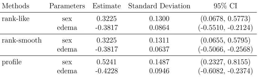
rank-smooth estimation method and the profile likelihood based estimation method.

There are consistent conclusions for both sex and edema from the three estimation

methods, that is, both sex and edema have the significant effects on the time to death

of patients, since the 95% confidence intervals for either sex or edema do not include

zero. The results also show that under either the rank-like estimation method or the

rank-smooth estimation method, the time to death of male patients is estimated to

reduce to e−0.3225 _{= 0}_._{7243 of those female patients, and if edema is present among}

the patients, the time to death is estimated to reduce to e−0.3817 _{= 0}_._{6827 of those}

without edema. Under the profile likelihood based estimation method, the time to

death of male patients is estimated to reduce to e−0.5241 _{= 0}_._{5921 of those female}

patients, and the time to death of patients with edema is estimated to reduce to

e−0.4228 = 0.6552 of those without edema.

Table 2.3 Estimates, SD and 95% CI of estimated parameters for the PBC data from AP-AFT model, under rank-like estimation method, rank-smooth estimation method and profile likelihood based estimation method

Methods Parameters Estimate Standard Deviation 95% CI

rank-like sex 0.3225 0.1300 (0.0678, 0.5773) edema -0.3817 0.0864 (-0.5510, -0.2124)

rank-smooth sex 0.3225 0.1311 (0.0655, 0.5795) edema -0.3817 0.0637 (-0.5066, -0.2568)

profile sex 0.5241 0.1487 (0.2327, 0.8155) edema -0.4228 0.0946 (-0.6082, -0.2374)

Figure 2.4 shows the nonlinear effects of the risk factors on the time to death

of patients. Both bilirubin and albumin have the nonliner significant effects on the

time to death of patients. Along with the increase of bilirubin, the time to death of

(39)

0 5 10 15 20 25

−5

−4

−3

−2

−1

0

bilirubin

f(bilir

ubin)

rank−smooth

95% CI of rank−smooth profile

95% CI of profile

2.0 2.5 3.0 3.5 4.0 4.5

−2

−1

0

1

2

3

albumin

f(alb

umin)

rank−smooth

95% CI of rank−smooth profile

95% CI of profile

Figure 2.4 Estimated nonlinear terms g1(bilirubin) and g2(albumin) obtained from rank-smooth estimation method and profile likelihood based estimation method along with their 95% confidence intervals

tend to have higher death probability than those with low level of bilirubin. We also

(40)

2.7 Discussion and Conclusion

In this chapter, we have proposed an additive partial AFT model, and its

corre-sponding estimation methods based on either the rank-smooth method or the profile

likelihood method. The simulation studies show the good performance of the

pro-posed methods. The main difference between the rank-smooth estimation method and

the rank-like estimation method is that the variance of the estimated parameters are

different. The rank-like estimation method used the the resampling techniques while

the other one used the induced smooth techniques. Furthermore, comparing with

the rank-smooth estimation method, the variance estimation of parameters based on

the profile likelihood based method is easy and straightforward, since the variance of

estimated parameters can be obtained through the inverse of the second derivative of

the kernel smoothed profile likelihood function. However, with the increase of sample

size, it may need more time than the rank-smooth method. In summary, we suggest

to using either the rank-smooth method or the profile likelihood method in practice

when sample size is moderate, and otherwise, the rank-smooth estimation method is

(41)

Chapter 3 Profile Likelihood based Estimation Method

for the Accelerated Failure Time Mixture

Model with Latent Subgroups

3.1 Abstract

In randomized clinical trials, subgroup analysis is very important and popular. Latent

subgroups arise since we can only know the subgroup membership in the treatment

set, and we know nothing about subgroup membership in the control set.

Biologi-cal efficacy, related to the subgroup of patients who benefit from the treatment, is

an important index for researchers to evaluate the treatment effects in the

treat-ment set. In this chapter, we develop a new estimation method for the

semipara-metric accelerated failure time mixture model with a latent subgroup based on the

expectation-maximization algorithm and the profile likelihood estimation method.

Simulation studies show that the proposed method is comparable to the existing

E-BJ algorithm, which incorporates a weighted Buckley-James optimization in the

maximization step. For illustration, we apply the proposed method to pregnancy data

obtained from Medicaid billing records, birth certificates, Department of Education,

(42)

3.2 Introduction

The PH model and the AFT model are the two most popular survival models in

fitting the right censored data. There are broad investigations into the estimation

methods for the AFT model. Miller [40] proposed the least square estimation method

to estimate the parameters in the AFT model. Buckley and James [7] developed a

least square estimation method based on the modified normal equations. Jin, Lin and

Ying [26] proposed one least square estimation method based on the Buckley-James

estimating equation. Tsiatis [56] used the linear rank test technique to estimate the

parameters of the AFT model. Wei, Ying and Lin [61] also used the linear rank

statistics as estimating functions for the regression parameters. Zeng et al. [70]

proposed an approximate nonparametric maximum likelihood method for the AFT

model. This method can be easily used to estimate the variance of parameters through

the inverse of the second derivative of the kernel-smoothed profile likelihood function.

In randomized clinical trials, subgroup analysis is very important and popular,

since it pertains to the assessment of treatment effects for a specific end point in

sub-groups of patients defined by baseline characteristics [58]. We focus on the situation

where patients who are treatable or not treatable do not receive any allocated

treat-ment in the control set. In comparison, patients in the treattreat-ment set may or may not

receive the treatment based on the baseline characteristics. For example, based on

race (African American and White), participants are randomized into two sets:

treat-ment set (all are African American) and control set (all are White) to test prostate

cancer. The participants with positive prostate biopsy are classified as treatable

sub-jects, and untreatable subjects are those without positive prostate biopsy. Whether

the participants are treatable subjects or not is not influenced by the randomization.

Treatable subjects in the treatment set belong to treatable subgroup A. The

untreat-able subjects in the treatment set belong to untreatuntreat-able subgroup B. Whether the

Measuring Strategic Communications

University of South Carolina

Scholar Commons

Semiparametric Estimation Methods For Complex

Accelerated Failure Time Model

Yinding Wang

SEMIPARAMETRIC ESTIMATION METHODS FOR COMPLEX ACCELERATED

FAILURE TIME MODEL

Acknowledgments

Abstract

Table of Contents

List of Tables

List of Figures

Chapter 1

Introduction

PH Model

AFT Model

Mixture Cure Model

Semiparametric PH Mixture Cure Model

Semiparametric AFT Mixture Cure Model

Chapter 2

Semiparametric Estimations for Additive

Partial Accelerated Failure Time Models

Rank-smooth estimation method

Profile Likelihood Based Estimation Method

Chapter 3

Profile Likelihood based Estimation Method

for the Accelerated Failure Time Mixture

Model with Latent Subgroups