Measuring Strategic Communications

(1)

University of South Carolina

Scholar Commons

Theses and Dissertations

2016

Modeling Embankment Breach Due To

Overtopping

Ali Asghari Tabrizi

University of South Carolina

Follow this and additional works at:https://scholarcommons.sc.edu/etd Part of theCivil Engineering Commons

This Open Access Dissertation is brought to you by Scholar Commons. It has been accepted for inclusion in Theses and Dissertations by an authorized administrator of Scholar Commons. For more information, please [email protected].

Recommended Citation

(2)

M

ODELING EMBANKMENT BREACH DUE TO OVERTOPPING

by

Ali Asghari Tabrizi Bachelor of Science

Isfahan University of Technology, 2006 Master of Science

Shiraz University, 2009 Master of Science

University of California Los Angeles, 2011

Submitted in Partial Fulfillment of the Requirements For the Degree of Doctor of Philosophy in

Civil Engineering

College of Engineering and Computing University of South Carolina

2016 Accepted by:

M. Hanif Chaudhry, Major Professor Jasim Imran, Committee Member Shamia Hoque, Committee Member

Jamil Khan, Committee Member

(3)

(4)

D

EDICATION

(5)

A

CKNOWLEDGEMENTS

(6)

A

BSTRACT

Despite numerous embankment failures around the world, in-depth assessments as well as reliable, comprehensive sets of data of such failures are limited. Detailed

(7)

bedload transport formula is the main component. A comparison between the simulated and observed breach outflow hydrograph shows that the simulations and observations are in better agreement by using the Meyer-Peter and Muller (M.P.M.) formula than the Ashida and Michiue (A.M.) formula. However, the A.M. formula predicts better the bed and water surface profiles after the initial failure stage. 3) For the Jet tests of cohesive samples with different levels of compaction, erodibility varies over a wide range and the effects of compaction energy and water content on the erodibility coefficients are

(8)

(9)

T

ABLE OF

C

ONTENTS

DEDICATION ... iii

ACKNOWLEDGEMENTS ... iv

ABSTRACT ...v

LIST OF TABLES ... xi

LIST OF FIGURES ... xii

CHAPTER 1INTRODUCTION ...1

1.1EARTHEN EMBANKMENT ...1

1.2MOTIVATION AND OBJECTIVES ...2

1.3ORGANIZATION OF THE DISSERTATION ...4

CHAPTER 2LITERATURE REVIEW ...5

2.1EARTHEN DAM FAILURE ...5

2.2SOIL ERODIBILITY MEASUREMENTS USING THE SUBMERGED JET TEST ...8

2.3EARTHEN LEVEE FAILURE ...10

CHAPTER 3EXPERIMENTAL STUDY ON EMBANKMENT BREACH DUE TO OVERTOPPING: EFFECTS OF COMPACTION ...11

3.1EXPERIMENTAL SETUP ...11

3.2TEST PROCEDURE ...12

3.3RESULTS ...14

(10)

4.3MODEL DESCRIPTION ...42

4.4RESULTS ...47

CHAPTER 5INVESTIGATING THE EFFECT OF COMPACTION CHARACTERISTICS ON THE ERODIBILITY OF A COHESIVE SOIL USING THE JET METHOD ...71

5.2RESULTS ...72

CHAPTER 6EXPERIMENTAL MODELING OF LEVEE FAILURE PROCESS DUE TO OVERTOPPING ...78

6.2MEASUREMENT METHODS ...79

6.3RESULTS ...81

CHAPTER 7EXPERIMENTAL MODELING OF EARTHEN LEVEE FAILURE BY OVERTOPPING: EFFECTS OF HYDRAULIC LOADS ...92

7.3MEASUREMENT METHODS ...94

7.4RESULTS ...94

7.5ANALYSIS OF BREACH CHARACTERISTICS ...98

CHAPTER 8EXPERIMENTAL MODELING OF EARTHEN LEVEE FAILURE BY OVERTOPPING: EFFECTS OF COMPACTION AND COHESION ...119

8.1EXPERIMENTAL DESCRIPTION ...119

(11)

8.4COMPARING COMPACTION WITH COHESION EFFECTS ...129

CHAPTER 9SUMMARY AND CONCLUSIONS ...159

9.1EXPERIMENTAL STUDY ON EMBANKMENT BREACH DUE TO OVERTOPPING: EFFECTS OF COMPACTION ...159

9.2NUMERICAL MODELING OF EARTHEN DAM BREACH DUE TO OVERTOPPING: INFLUENCE OF DIFFERENT MODEL PARAMETERS ...160

9.3INVESTIGATING THE EFFECT OF COMPACTION CHARACTERISTICS ON THE ERODIBILITY OF A COHESIVE SOIL USING THE JET METHOD ...161

9.4EXPERIMENTAL MODELING OF LEVEE FAILURE PROCESS DUE TO OVERTOPPING ...161

9.5EXPERIMENTAL MODELING OF EARTHEN LEVEE FAILURE BY OVERTOPPING: EFFECTS OF HYDRAULIC LOADS ...162

9.6EXPERIMENTAL MODELING OF EARTHEN LEVEE FAILURE BY OVERTOPPING: EFFECTS OF COMPACTION AND COHESION ...163

9.7RECOMMENDATIONS ...165

REFERENCES ...167

(12)

L

IST OF

T

ABLES

Table 3.1 Numerical cases by various modeling parameters ...26

Table 4.2 Averaged root mean square error for numerical cases with A.M. formula and M.P.M. formula ...52

Table 5.1 Soil sample properties used in Submerged Jet tests ...74

Table 7.1 Test data ...103

Table 7.2 RMSE of the breach shape predictions at different times ...103

(13)

L

IST OF

F

IGURES

Figure 3.1 Schematic diagram of the experimental tests (a) side view, (b) plan view ...27 Figure 3.2 Repeatability of the progressive failure process for Nb = 10 blows/layer

at: (a) t = 5 s; (b) 10 s; (c) 15 s; (d) 25 s; (e) 40 s; and (f) 60 s ...28 Figure 3.3 Breach evolution for different compaction efforts:

Nb = 0 (a); Nb = 10 (b); Nb = 20 (c); and Nb = 30 (d) ...29

Figure 3.4 Degradation rate of the embankment crest for different compaction levels ....30 Figure 3.5 Downstream hydrograph for different compaction efforts ...30 Figure 3.6 Correlation of normalized peak breach discharge and normalized dry density

of the embankment ...31 Figure 3.7 Correlation of normalized time to peak discharge and normalized dry density

of the embankment ...31 Figure 3.8 Comparison between experimental and empirical results of the breach outflow

hydrograph for: (a) Nb = 0; (b) Nb = 10; (c) Nb = 20; and (d) Nb = 30 ...32

Figure 3.8 (continued) Comparison between experimental and empirical results of the breach outflow hydrograph for: (a) Nb = 0; (b) Nb = 10; (c) Nb = 20; and (d) Nb

= 30 ...33 Figure 3.9 Time variation of dimensionless embankment crest height for different

compaction levels using Eq. (3.3) ...34 Figure 3.10 Comparison between experimental and empirical results of temporal changes

of normalized crest height for: (a) Nb = 0; and (b) Nb = 20 ...34

Figure 3.11 Time variation of dimensionless embankment length for different compaction levels using Eq. (3.4) ...35 Figure 3.12 Comparison between experimental and empirical results of temporal

(14)

Figure 3.13 Schematic diagram of proposed triangular model to predict the progressive

breach shape (image by author) ...36

Figure 3.14 Measured and predicted bed surface profiles using the triangular model for Nb = 20 at: (a) t = 10 s; (b) t = 25 s; (c) t = 40 s; and (d) t = 60 s ...37

Figure 3.15 Observed and predicted normalized crest height variation with time ...38

Figure 3.16 Outflow Characteristics vs. eroded volume ...38

Figure 3.17 Breach development time vs. eroded volume ...39

Figure 3.18 Time variation of dam crest level using the experimental data of no-compaction and the results of the mathematical model with different values of 𝛼𝛼₂ ...39

Figure 4.1 Breach outflow hydrograph according to experimental tests ...53

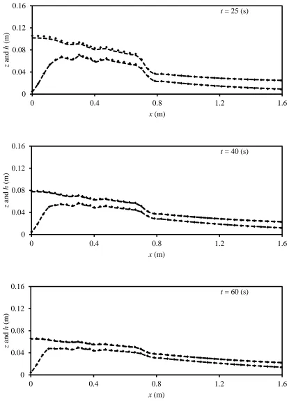
Figure 4.2 Embankment surface profile z (x) and water surface profiles h(x) at various times t for three experimental tests ...54

Figure 4.3 Averaged outflow hydrograph of the three tests ...56

Figure 4.4 Averaged embankment surface profiles z(x) of three tests at various times t ..56

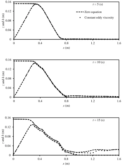
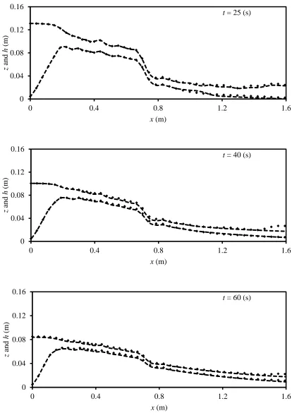
Figure 4.5 Turbulent model effect: simulated bed and water surface profiles at various times for Case 15 with constant eddy viscosity model and Case 16 with zero equation model ...57

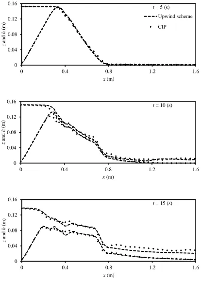
Figure 4.6 Finite difference approximations of advection terms effect: simulated bed and water surface profiles at various times for Case 1 with upwind scheme method and Case 9 with CIP method ...59

Figure 4.7 Suspended load effect: simulated bed and water surface profiles at various times for Case 1 with bedload and suspended load and Case 5 with bedload only ...61

Figure 4.8 Outflow hydrographs for Case 1 with bedload and suspended load and Case 5 with bedload only ...63

(15)

formula ...66 Figure 4.11 Bed and water surface profiles at various times t according to averaged

experimental tests and numerical simulations for Case 10 (A.M.) and 12 (M.P.M) ...68 Figure 4.12 Outflow hydrographs according to the averaged experimental tests and

simulations for Case 4 (M.P.M.) with Case 1 (A.M.) ...70 Figure 5.1 Submerged Jet test apparatus and the standard proctor compaction mold and

rammer ...74 Figure 5.2 Standard proctor compaction test curve ...75 Figure 5.3 Relationship of kd and 𝜏𝜏c from the Submerged Jet test results for three levels of

compaction and water content ...75 Figure 5.4 kd vs. water content for 25 B/L, 15 B/L, and 10 B/L compaction effort ...76

Figure 5.5 Averaged kd vs. water content for 25 B/L, 15 B/L, and 10 B/L compaction

effort ...76 Figure 5.6 Averaged τc vs. water content for 25 B/L, 15 B/L, and 10 B/L compaction

effort ...77 Figure 6.1 Plan view of experimental setup (dimensions are in meter) ...85 Figure 6.2 Front view of the proposed method for measuring the breach shape with

time ...85 Figure 6.3 Spatial variation of water surface velocity at different times ...86 Figure 6.4 Time series of breach width for the left and right bank of the breach (flow

direction in the channel is from left to right) ...86 Figure 6.5 Hydrographs of inflow to the flume, outflow from the downstream weir, and

outflow from the breach ...87 Figure 6.6 Time series of breach evolution (flow direction in the channel is from

right to left) ...87 Figure 6.7 Time series of water depth at breach location (flow direction in the channel is

(16)

Figure 6.9 Non-dimensional deepening and widening rate with time ...90 Figure 6.10 Correlation of deepening and widening rate with excess shear stress ...91 Figure 7.1 Time history of: (a) maximum breach depth; (b) top width of the breach; (c)

breach area along the centerline of the crest; and (d) total breach volume ....104 Figure 7.2 Breach evolution along the center of the levee crest ...105 Figure 7.3 Breach evolution for Test A3 (flow direction in the main channel is from right to left) ...107 Figure 7.4 Longitudinal profiles along the centerline of the pilot channel at different

times for Test A3 ...108 Figure 7.5 Breach top width for the downstream and upstream breach walls at different

times for Test A3 (centerline of the pilot channel is shown as dash line) ...109 Figure 7.6 Water surface velocity distribution for Test A3 at different times ...110 Figure 7.7 Weir flow and breach overflow hydrographs for all tests ...111 Figure 7.8 Comparison of experimental and empirical normalized breach top width with

time for: (a) Test A2; and (b) Test B3 ...112 Figure 7.9 Empirical results of normalized breach top width with time for all tests ...113 Figure 7.10 Comparison of experimental and empirical normalized maximum breach

depth with time for: (a) Test A3; and (b) Test B2 ...114 Figure 7.11 Empirical results of normalized maximum breach depth with time for all

tests ...115 Figure 7.12 Comparison of experimental and empirical normalized breach volume with

time for: (a) Test A2; and (b) for Test B1 ...116 Figure 7.13 Empirical results of normalized breach volume with time for all tests ...117 Figure 7.14 Comparison of the experimental and the predicted breach shape at different

times using the trapezoidal model for Test A3 ...118 Figure 8.1 Experimental setup in: (a) schematic view; and (b) plan view. Location of the

(17)

Figure 8.3 Time history of the maximum breach depth along the centerline of the levee

crest for four levels of compaction ...132

Figure 8.4 Breach profiles along the crest centerline at various times for: (a) Nb = 0; (b) Nb = 2; (c) Nb = 4; and (d) Nb = 10 ...133

Figure 8.5 Breach evolution for test with NB = 0 at t = 10, 20, 25, 30, 35, and 40 s ...135

Figure 8.9 Time series of longitudinal bed profiles along the centerline of the pilot channel for: (a) Nb = 0; (b) Nb = 2; (c) Nb = 4; and (d) Nb = 10 ...139

Figure 8.10 Cumulative breach eroded volume with time for four levels of compaction ...141

Figure 8.11 Time series of the submerged area along the centerline of the levee crest for four levels of compaction...141

Figure 8.12 Weir flow and breach overflow for four levels of compaction: (a) Nb = 0; (b) Nb = 2; (c) Nb = 4; and (d) Nb = 10 ...142

Figure 8.13 Correlation of the breach deepening rate along the crest centerline and the excess shear stress on the bed ...144

Figure 8.14 Correlation of the breach widening rate along the crest centerline and the excess shear stress on the sidewalls ...144

Figure 8.15Comparisons of observed and predicted normalized deepening rate ...145

Figure 8.16Comparisons of observed and predicted normalized widening rate ...145

Figure 8.17Normalized eroded load versus the excess Shields number for different tests ...146

Figure 8.18Comparisons of observed and predicted normalized eroded volume ...146

Figure 8.19Breach evolution for Test 5 at t = 5, 20, 40, 60, 80, and 110s ...147

Figure 8.20Breach evolution for Test 6 at t = 10, 40, 80, 120, 150, and 170s ...148

(18)

Figure 8.22Breach evolution for Test 8 at t = 1, 5, 10, 15, 19, and 21 min ...150 Figure 8.23Time changes of breach top width for levees with different cohesion ...151 Figure 8.24Time changes of breach depth for levees with different cohesion ...151 Figure 8.25Breach profiles at different times for: (a) Test 5; (b) Test 6; (c) Test 7; and

and (d) Test 8 ...152 Figure 8.26Weir flow and breach overflow for four levels of cohesion: (a) Test 5; (b)

Test 6; (c) Test 7; and (d) Test 8 ...154 Figure 8.27Envelope curves of breach top width for different levels of compaction and

cohesion ...156 Figure 8.28Envelope curves of breach depth for different levels of compaction and

cohesion ...156 Figure 8.29Envelope curves of breach eroded volume for different levels of compaction

and cohesion ...157 Figure 8.30Envelope curves of breach submerged area for different levels of compaction and cohesion ...157 Figure 8.31Envelope curves of breach total area for different levels of compaction

(19)

CHAPTER

1 I

NTRODUCTION

1.1Earthen Embankment

Embankment structures are volume of erodible (earthen) and/or non-erodible (concrete) material built by humans or formed naturally. These are used for flood protection and water storage for drinking and irrigation, energy production, and recreation purposes. The number of extreme hydrological events, e.g. hurricanes, rainstorms, and typhoons, has increased in recent years due to climate change (Kakinuma and Shimizu, 2014), thereby increasing the risk of embankment failure and flooding. Earthen embankments are emplaced to control water flow and provide protection from flood. They may be classified based on their orientation with respect to the flow direction, namely, 1) built along a river to prevent overflow, called a levee or dike, and 2) built perpendicular to the general flow direction, called a dam.

Flood disasters are common worldwide, due to levee breach and occasionally dam failure resulting in fatalities and considerable economic losses. Failure of earthen

embankments may be due to various reasons, such as overtopping, seepage, internal erosion and piping, and slope instability. However, overtopping is the most common cause of the embankment failure (ASCE/EWRI Task Committee on Dam/Levee

(20)

An accurate prediction of the embankment failure by overtopping (i.e., breach shape, breach outflow and flow field) is necessary for emergency planning, proper risk assessment and management, and protection measures. Estimating the soil erodibility by flowing water is an essential step in studying, modeling, and predicting earthen

embankment failures. An embankment breach is influenced by both hydraulic load and geotechnical properties of the embankment material (Schmocker and Hager, 2012). The most important geotechnical parameters affecting the embankment erodibility are: grain size distribution which implies cohesion and plasticity, compaction energy, and water content.

1.2Motivation and Objectives

Despite numerous examples of embankment breaching around the world (e.g., the Elbe flood disaster in 2002 and 2013, the New Orleans flood in 2005, and most recently the October 2015 flood in the Midlands area of South Carolina), in-depth assessments as well as useful data of such failures are limited due to a variety of reasons, including the lack of proper documentation and organization in data collection. Furthermore, detailed understanding of the embankment failure process and the dominant parameters affecting the failure is a crucial step in predicting and modeling the breach process for risk

assessment and preparing emergency plans and hazard maps. The objectives of the present study are:

(21)

breach, downstream outflow hydrograph, and rate of erosion of the embankment crest for different compactions. The main goal is to develop non-dimensional relationships for the crest height and embankment bottom length as a function of time and compaction energy based on the measured data and to develop a simple relationship which enables the prediction of the progressive breach shape.

2) To model the overtopping failure of the homogenous, compacted, non-cohesive embankment dam case, applying the iRIC-Nays2D softwaredeveloped by Foundation of Hokkaido River Disaster Prevention Research Center to study the influence of different model parameters, i.e. turbulence model,

finite-difference approximation of the advection term, sediment transport type, and bedload formula, on model prediction.

3) To measure the erodibility of the cohesive (sandy loam) soil samples for three levels of compaction and water content (i.e., low, medium, and high) assuming erosion detachment model using the Submerged Jet method.

4) To conduct a series of levee embankment overtopping experiments in which the levee is aligned parallel to the dominant flow direction, similar to field conditions and quantitatively determine the effects of hydraulics loads, compaction level, and cohesion on the failure process of overtopped homogenous levees (i.e., breach evolution using a sliding-rod technique, measurement of breach outflow, and water surface velocity distributions using a particle-image velocimetry method). Erodibility coefficients in both vertical and horizontal directions are estimated from the experimental results to assess the compaction effects and the

(22)

formulas are proposed. Envelope curves of breach characteristics (e.g., breach top width and breach depth with time) are also developed from experimental results for a range of compaction and cohesion.

1.3 Organization of the Dissertation

This dissertation has nine chapters. Characteristics and importance of the embankment structures and their failure modes are presented in this chapter. The

motivation and objectives of the study are identified. The background and the literatures relevant to the current study are reviewed in Chapter 2. The experimental setup,

(23)

CHAPTER 2 L

ITERATURE

R

EVIEW

Literature on earthen dam failure (experimental and numerical investigations), soil erodibility measurements using the Submerged Jet test, and earthen levee failure are reviewed in this chapter.

2.1 Earthen Dam Failure

Morris (2009) and a forum paper by the ASCE/EWRI Task Committee on Dam/Levee Breaching (2011) summarized the state of the knowledge on earthen embankment breaching. Wahl (2007) reviewed the laboratory investigations on embankment breach process conducted over the past decades. Furthermore, Schmocker and Hager (2009) and Schmocker (2011) have summarized the past hydraulic modeling of embankment breach due to overtopping.

Experimental Investigations

(24)

over an embankment: 1) subcritical flow from the reservoir to the upstream portion of the embankment crest; 2) supercritical flow on the remainder of the crest; and 3) rapidly accelerating turbulent supercritical flow on the downstream slope of the embankment.

Coleman et al. (2002) investigated the overtopping failure of non-cohesive

homogeneous embankments subject to a constant-head reservoir. The evolution of breach was discussed and non-dimensional relationships for the breach cross-section width and breach discharge were presented. Hanson et al (2003) defined four stages for the erosion process based on the observations on large-scale overtopping failure experiments on cohesive embankment. Chinnarasri et al. (2003) analyzed the results from nine

experimental runs of overtopping failure of non-cohesive embankments with variations of the downstream slope of the dike. They classified the progressive failure of the

embankment into four stages, namely: 1) small erosion on the embankment crest; 2) slope sliding failure; 3) wavelike-shape embankment profile; and 4) large wedge of eroded embankment with a small bed slope along the flume. The degradation rate of the dike crest was found to be dependent on and directly correlated to the downstream slope. Dupont et al. (2007) performed an experimental study of the progressive breaching of an overtopped dam. Just before the actual overtopping, they observed sliding at the lower portion of the downstream slope because of water seepage. Then, the erosion advances from the downstream face to the upstream face of the embankment by rotation of the downstream face around a pivot point. Antidunes are then formed on the downstream face and the embankment profile stabilizes.

(25)

breach section develops vertically at the beginning and enlarges further laterally. They presented non-dimensional relations for the peak outflow through the breached

embankment and breach deformation time from their measured data and a number of historical dataset. Schmocker and Hager (2009) conducted a series of laboratory tests on non-cohesive plane dike breach to examine model limitations regarding the test

repeatability, side wall effects, and scale effects. More recently, Schmocker and Hager (2012) performed several hydraulic model tests to investigate the effects of dike dimension, sediment diameter, and inflow discharge on the failure of the overtopped embankments. They presented non-dimensional relations for the maximum dike height, dike volume, and maximum breach discharge.

Numerical Investigations

According to the forum paper by the ASCE/EWRI Task Committee on Dam/Levee Breaching (2011), embankment breach models are classified as parametric, simplified physically-based, or detailed physically based. Parametric models use regression equations that are developed based on the data from historic dam failures (Kirkpatrick 1977; Hagen 1982; Von Thun and Gillette 1990; Xu and Zhang 2009; Pierce et al. 2010).

(26)

Detailed physically-based models of breaching process are relatively recent and include one-dimensional, depth-averaged two-dimensional and three-dimensional hydrodynamic models and various sediment transport models (Tingsanchali and

Chinnarasri 2001; Wang and Bowles 2006; Wang et al. 2008; Cao et al. 2011). There is considerable amount of diversity in these models in terms of solution methods, numerical accuracy, sediment entrainment and transport modeling. The depth-averaged 1D and 2D models are computationally efficient and preferable over 3D models due to the

requirement of considerable amount of computational resources and run time for the application of the latter. For both 2D and 3D Reynolds-averaged models, local

equilibrium in turbulence and sediment transport are assumed. These assumptions may lead to inaccurate results due to rapid changes in bed level and high sediment

concentration during breach evolution. Systematic sensitivity studies of numerical models are necessary to study the effect of turbulence models, choice of numerical scheme, sediment transport formula, and mode of sediment transport on model predictions.

2.2 Soil Erodibility Measurements Using the Submerged Jet Test

Estimating the soil erodibility by flowing water is an essential step in studying, modeling, and predicting embankment failures which can be widely used in emergency action plans and risk assessments. Furthermore, estimating erodibility of cohesive soil is more

complex because of the large number of parameters controlling the erosion behavior and the difficulty of estimating these parameters.

(27)

the critical shear stress. The detachment model is a fundamental and widely accepted equation used in characterizing erodibility for embankment overtopping (Temple et al., 2005) and has been used by several investigators (Hutchinson, 1972; Foster et al., 1977; Dillaha and Beasley. 1983; Temple, 1985; Hanson, 1989; Stein and Nett, 1997; Wan and Fell, 2004).

𝜀𝜀 =𝑘𝑘𝑑𝑑(𝜏𝜏𝑒𝑒− 𝜏𝜏𝑐𝑐) (2.1)

where 𝜀𝜀 is the erosion rate (m/s), 𝑘𝑘_𝑑𝑑 is the erodibility or detachment coefficient (m3/N-s),

𝜏𝜏𝑒𝑒 is the hydraulically applied shear stress (Pa), and 𝜏𝜏𝑐𝑐 is the critical shear stress (Pa).

(28)

2.3 Earthen Levee Failure

An accurate prediction of the levee failure process by overtopping (i.e., breach shape, breach outflow, and flow field) is necessary for emergency planning, risk assessment and management, and protection measures. Estimating the soil erodibility by flowing water is an essential step in studying, modeling, and predicting earthen embankment failures. Characterizing erodibility of levees becomes even more complicated considering downward and lateral directions of erosion. Majority of the levee breach experiments have been conducted in flumes with the flow direction perpendicular to the embankment (Wahl 2007).

(29)

CHAPTER 3 E

XPERIMENTAL

S

TUDY ON

E

MBANKMENT

B

REACH DUE TO

O

VERTOPPING

:

E

FFECTS OF

C

OMPACTION∗

The effects of the soil compaction energy on the plane embankment breach process due to overtopping are investigated in this chapter. Experiments were conducted in the Hydraulics Laboratory, University of South Carolina, considering four levels of compaction energy and a simple trapezoidal shape for embankments consisting of uniform sand. Of particular interest was time evolution of the breach, downstream outflow hydrograph, and degradation rate of the embankment crest for different

compactions. The main goal was to develop non-dimensional relationships for the crest height and embankment bottom length as a function of time and compaction energy based on the measured data and ultimately to introduce a simple relationship which enables the prediction of the progressive breach shape.

3.1 Experimental Setup

The experiments were carried out in a 6.1 m long, 0.25 m deep, and 0.2 m wide horizontal rectangular flume. Figure 3.1 shows the schematic diagram of the plan and side view of the setup. One sidewall of the flume is made of Plexiglas to enable video recording of the longitudinal breach evolution process, i.e., changes of sediment surface profiles with time. Recording was done using a high-definition (HD) video camera, at a

∗_{Asghari Tabrizi, A., Elalfy, E., Elkholy, M., Chaudhry, M.H., Imran, J. 2016. “Effects of compaction on}

(30)

resolution of 1280 x 720 pixels, facing the cross profile of the embankment. To visually differentiate the bed and water surfaces, dye was injected into water close to the upstream face of the embankment during the breach evolution. The intake length was 0.5 m and a flow straightener honeycomb was used to reduce the inflow turbulence. A basin was located at the downstream end of the flume to collect the water discharging from the breached embankment. The inflow discharge was kept constant at 0.0005 m3_/s.

3.2 Test Procedure

Prior to the embankment overtopping tests, Standard Proctor Compaction tests (ASTM D698) were carried out to determine the optimum water content of the homogenous, non-cohesive soil (i.e., sand only) used in the experiments. The optimum water content was found to be 5.2% and the corresponding maximum dry unit weight, 𝛾𝛾_𝑑𝑑_,_{𝑚𝑚𝑚𝑚𝑚𝑚}, is 15.44 kN/m3. The trapezoidal earthen embankments of uniform sand with the mean diameter of 0.55 mm were placed 3.1 m downstream from the intake in the streamwise direction. The upstream toe of the embankment was considered to be the origin of the coordinate

system. The dimensions of the embankment for all the tests were: embankment height = 0.15 m, embankment width = 0.2 m, embankment crest length = 0.1 m, upstream and downstream embankment slopes, s (V: H) = 1:2. Four different cases were considered by applying different levels of compaction to build the embankments using a 4.54 kg

(31)

compaction), 10, 20, and 30. For each layer, the soil surface was trimmed and levelled to 5 cm precisely after the compaction. After placing and compacting the third layer, the upstream and downstream faces of the embankment were trimmed carefully to reach the final trapezoidal shape. The seepage through the embankment was controlled and reduced by a thin clay layer with low permeability placed on the upstream face of the

embankment. The parameters for the test cases are presented in Table 3.1. The compaction energy is denoted by 𝐶𝐶_𝑒𝑒.

To reduce the contact time between water and the upstream embankment face prior to overtopping and in turn to reduce the seepage through the embankment, the reservoir was filled at a relatively fast rate using two additional hoses along with the pump inflow. As the water surface reached about 5 cm below the embankment crest, the extra supply of water was cut off (i.e., the inflow was provided by the pump only). Small initial waves generated due to the rapid filling of the reservoir dissipated after a few seconds and the water surface was almost horizontal when the overtopping started. The valve for the dye container was opened slightly to add color to the water (the inflow from the color container was negligible). The starting time of the failure process was

considered to be the time when the water surface reached the upstream edge of the embankment crest. Furthermore, sand-cone tests were conducted to determine the dry unit weight of the embankment material for each compaction level. The dry unit weights,

𝛾𝛾𝑑𝑑, were found to be 13.35, 14.75, 15.46, and 15.47 kN/m3 for Nb = 0, 10, 20, and 30,

respectively.

Because of the limited width (i.e., 0.2 m), all of the embankments were

(32)

et al. 2010, Schmocker and Hager 2009). So, the longitudinal embankment profile observed through the Plexiglas side of the flume represents the entire embankment. As observed by Schmocker and Hager (2009), the sidewall effect was negligible. During the breach evolution, the bed surface profiles were recorded by an HD camera. The videos were first converted into frames for one-second time intervals and then the longitudinal bed surface profiles were obtained by digitizing the frames with an expected error of ±1 mm. The breach outflow was measured at the downstream end of the flume using the volumetric technique. Each test was repeated at least three times to confirm the repeatability of the tests. With the repeatability confirmed, the measured temporal changes of longitudinal embankment bed profile were averaged and analyzed.

3.3 Results

Repeatability

To ensure the reliability of the measurements, the repeatability of the tests was checked by considering both the embankment bed evolution and also the breach outflow

hydrograph for all four cases of compaction prior to analyzing the results. Each case was repeated at least three times using identical conditions to reduce uncertainty of the measured data. Figure 3.2 shows the development of the breach with time for three different runs for the case with Nb = 10 blows/layer. Bed surface profiles of different runs

(33)

found to have better repeatability as compared to the cases with compaction. The averaged RMSE, over the time and over the repetitions, was calculated for all the test cases, and was about 0.005 m for all of the test cases for the bed evolution. A better repeatability was also observed for the breach hydrograph for the case with no

compaction (RMSE = 0.001 m3s-1m-1 for no-compaction case and RMSE = 0.002 m3s-1m -1_{for the compacted cases). The better repeatability for the case with no-compaction may}

be due to the fact that surface erosion was the only mechanism that governed the failure process, while for the cases with compaction both head cut erosion (i.e., irregular detachment of soil chunks) and surface erosion controlled the failure process.

Breach Shape Evolution

Figure 3.3 shows the progressive failure of the embankment for different levels of

compaction, Nb = 0, 10, 20, and 30. A relatively similar erosion process was observed for

the overtopped embankments with different compaction efforts, but the failure process was faster in the case of non-compacted embankment. The starting time of the

overtopping process, i.e. t = 0 s, is the time when the water surface at the reservoir reached the upstream edge of the crest. The upstream and downstream faces of the

embankment remained relatively intact until about t = 5 s and 15 s for Nb = 0 and Nb = 10,

(34)

on the fixed upstream slope. At around t = 60±5 s (as the time step of image processing was 5 s), the erosion process reached an equilibrium condition (i.e., when the bed and water surface profiles remained almost unchanged) and the stable embankment surface profiles were formed with a relatively small downstream slope. The observations of the temporal advance of embankment erosion in the current study are consistent with the erosion processes described by Dupont et al. (2007) and Schmocker and Hager (2009).

Some irregular bed surface profiles from t = 25 to 40 s were observed on the downstream face of the compacted embankments as compared to the non-compacted one. This may be due to the effects of combined head cut and surface erosion processes for the compacted embankments, while the surface erosion is the only mechanism during the failure of the non-compacted embankment. The equilibrium embankment crest height (i.e., the height of the crest at the end of the failure process when the bed and water surface profiles remained almost unchanged) increased with compaction effort, with no major differences between Nb = 20 and Nb = 30 since the soil dry unit weight reached its

maximum value (based on the standard proctor compaction test) for Nb = 20.

Figure 3.4 shows the variation of the crest degradation rate with time for various levels of compaction. The crest degradation plots of compacted embankments are generally

similar. For the non-compacted embankment, the degradation rate of the crest increased rapidly and reached its maximum value (Drate,max = 0.0035 m/s) during the early stage of

(35)

with a milder slope such that the final degradation rates were higher as compared to the non-compacted embankment.

Downstream Hydrograph

The discharge from the breached embankment constructed with different compaction levels was measured at the downstream end of the flume (Figure 3.5). The starting time of the hydrographs is the time when the water reached the end of the flume. The breach discharge increased at a fast rate during initial stages of failure until it reached its peak. Then, it decreased with a smaller rate until it was constant and equal to the inflow

discharge. A minor rise was observed on the falling limb of the hydrographs at around t = 15 s. This minor increase may be due to the release of water stored behind the

embankment when the headcut erosion reached the upstream edge of the crest. The amplitude of the second rise increased with the compaction level. This was consistent with the experimental observation that the dominance of the headcut erosion mechanism increased with the compaction level compared to the surface erosion mechanism and resulted in more abrupt water release. It was found that the peak discharge decreased while the time to peak increased with the compaction level. As mentioned previously, the embankment overtopping tests were run for different number of blows per layer, Nb. To

have a more general variable representing compaction, normalized dry density, 𝛼𝛼=

𝛾𝛾𝑑𝑑/𝛾𝛾𝑑𝑑,𝑚𝑚𝑚𝑚𝑚𝑚 , is used in this study, corresponding to each Nb where 𝛾𝛾_𝑑𝑑 is the dry unit

weight of the embankment material obtained from sand-cone test and 𝛾𝛾_𝑑𝑑_,_{𝑚𝑚𝑚𝑚𝑚𝑚} is the maximum dry unit weight from the standard proctor compaction test. The relationship

between these two variables is 𝛼𝛼 = 0.045𝑁𝑁_𝑏𝑏0.37+ 0.86 with R2_{= 0.95. The fitted}

(36)

normalized dry density are derived as 𝑞𝑞_{𝑝𝑝𝑒𝑒𝑚𝑚𝑝𝑝}⁄𝑞𝑞_{𝑏𝑏𝑚𝑚𝑏𝑏𝑒𝑒} = −12.80α+ 17.42 (R2_{of 0.93) and} 𝑡𝑡𝑝𝑝𝑒𝑒𝑚𝑚𝑝𝑝⁄𝑡𝑡0 = 16.62𝛼𝛼 −10.74 (R2of 0.64), respectively (Figure 3.6 and Figure 3.7), where

𝑞𝑞𝑝𝑝𝑒𝑒𝑚𝑚𝑝𝑝 is peak discharge per unit width, 𝑞𝑞𝑏𝑏𝑚𝑚𝑏𝑏𝑒𝑒 is constant inflow discharge to the flume

per unit width, 𝑡𝑡_{𝑝𝑝𝑒𝑒𝑚𝑚𝑝𝑝} is time to peak, and 𝑡𝑡₀ is the travel time of a wave in the upstream

reservoir defined as 𝑡𝑡₀ = 𝐿𝐿_𝑜𝑜⁄�𝑔𝑔ℎ_𝑜𝑜, where Lo is the length of the upstream reservoir and

ho is the initial height of water in the upstream reservoir.Although there are only limited

data points in these figures, a clear trend can be observed. The last two data points in these figures have almost the same α value since the optimum compaction level was reached with Nb = 20 and further compaction did not change the value of α significantly.

Using the experimental results of the breach outflow and regression analysis, two non-dimensional fitted equations are developed that express the rising limb and the falling limb of the breach outflow hydrograph separately for different levels of compaction and they are presented as

𝑞𝑞𝑟𝑟𝑟𝑟𝑏𝑏𝑟𝑟𝑟𝑟𝑟𝑟⁄𝑞𝑞𝑏𝑏𝑚𝑚𝑏𝑏𝑒𝑒 = (−6.4𝛼𝛼+ 7.1)(𝑡𝑡 𝑡𝑡⁄ 0) for 𝑡𝑡 ≤ 𝑡𝑡𝑝𝑝𝑒𝑒𝑚𝑚𝑝𝑝 (3.1)

𝑞𝑞𝑓𝑓𝑚𝑚𝑓𝑓𝑓𝑓𝑟𝑟𝑟𝑟𝑟𝑟⁄𝑞𝑞𝑏𝑏𝑚𝑚𝑏𝑏𝑒𝑒 = (35.1𝛼𝛼 −11.5)(𝑡𝑡 𝑡𝑡⁄ 0)−0.8 for 𝑡𝑡> 𝑡𝑡𝑝𝑝𝑒𝑒𝑚𝑚𝑝𝑝 (3.2)

where 𝑞𝑞_{𝑟𝑟𝑟𝑟𝑏𝑏𝑟𝑟𝑟𝑟𝑟𝑟} is the unit discharge on the rising limb of the hydrograph and 𝑞𝑞_{𝑓𝑓𝑚𝑚𝑓𝑓𝑓𝑓𝑟𝑟𝑟𝑟𝑟𝑟} is the

(37)

results for different levels of compaction as shown in Figure 3.8. The predicted and the experimental results correlate well for all the compaction levels with the average RMSE of 0.31, except some minor differences for the case with Nb = 20.

Crest Height

The temporal changes of the maximum embankment height were measured for different normalized dry densities. Using regression analysis, the best fit curve for these changes is obtained as

𝑍𝑍𝑐𝑐𝑟𝑟𝑒𝑒𝑏𝑏𝑐𝑐⁄𝑍𝑍𝑟𝑟𝑟𝑟𝑟𝑟𝑐𝑐𝑟𝑟𝑚𝑚𝑓𝑓 = �6.34 × 10−5(𝑡𝑡 𝑡𝑡⁄ 0)3−0.0014(𝑡𝑡 𝑡𝑡⁄ 0)2−0.024(𝑡𝑡 𝑡𝑡⁄ 0) +

1

𝛼𝛼−2.502�(𝛼𝛼)−2.502 (3.3)

where 𝑍𝑍_{𝑐𝑐𝑟𝑟𝑒𝑒𝑏𝑏𝑐𝑐} = crest height at each time step, 𝑍𝑍_{𝑟𝑟𝑟𝑟𝑟𝑟𝑐𝑐𝑟𝑟𝑚𝑚𝑓𝑓} = initial height of the crest before overtopping, and 𝑡𝑡 = time from starting of overtopping. The fitted equation (Eq. 3.3) was chosen as a 3rd order polynomial equation since it satisfactorily describes the physical phenomenon which includes acceleration and deceleration of the crest height changes. Figure 3.9 shows the variation of the normalized crest height, 𝑍𝑍_{𝑐𝑐𝑟𝑟𝑒𝑒𝑏𝑏𝑐𝑐}⁄𝑍𝑍_{𝑟𝑟𝑟𝑟𝑟𝑟𝑐𝑐𝑟𝑟𝑚𝑚𝑓𝑓}, with normalized time, 𝑡𝑡 𝑡𝑡⁄ ₀, for different compaction levels using Eq. 3.3. For a given normalized time, differences between the normalized crest height decreased with the compaction effort such that increasing the compaction beyond Nb = 20 (which

(38)

compared for different levels of compaction. Except for some small deviations, the measured data from laboratory experiments and the estimated ones from Eq. 3.3 are in satisfactory agreement with R2_{values greater than 0.94 for all the cases. Figures 3.10(a}

and b) show the comparison between the empirical and experimental results for Nb = 0

(R2 of0.94) and 20 (R2 of 0.99), respectively.

Embankment Length

The development of the embankment bottom length (i.e., distance from the upstream toe to the downstream toe of the embankment at each time step), 𝐿𝐿_{𝑏𝑏𝑚𝑚𝑏𝑏𝑒𝑒}, was measured during the failure process of the overtopped embankments. The empirical relation of the

normalized embankment length as a function of time and dry unit weight is obtained by regression analysis as

𝐿𝐿𝑏𝑏𝑚𝑚𝑏𝑏𝑒𝑒⁄𝐿𝐿𝑟𝑟𝑟𝑟𝑟𝑟𝑐𝑐𝑟𝑟𝑚𝑚𝑓𝑓 = [−4.95 × 10−4(𝑡𝑡 𝑡𝑡⁄ 0)3+ 1.56 × 10−2(𝑡𝑡 𝑡𝑡⁄ 0)2 −5.99 × 10−2(𝑡𝑡 𝑡𝑡⁄ 0) +

1.01](𝛼𝛼)−0.5 _(3.4)

where 𝐿𝐿_{𝑟𝑟𝑟𝑟𝑟𝑟𝑐𝑐𝑟𝑟𝑚𝑚𝑓𝑓} = initial length of the embankment before overtopping. Similar to the crest height regression analysis, a 3rd order equation better explains the actual changes of the embankment bottom length. Figure 3.11 shows the time variation of the normalized embankment length, 𝐿𝐿_{𝑏𝑏𝑚𝑚𝑏𝑏𝑒𝑒}⁄𝐿𝐿_{𝑟𝑟𝑟𝑟𝑟𝑟𝑐𝑐𝑟𝑟𝑚𝑚𝑓𝑓}, for different compaction levels by applying Eq. 3.4. The deviation between the curves at a given time step decreases with increasing the compaction and the compaction effect becomes insignificant beyond Nb = 20. Figures

(39)

Modeling Evolution of the Breach

As mentioned previously, when the water overtopped the embankment, first, the crest eroded from the downstream to the upstream edge. With time, a wedge-shaped embankment formed with the downstream face rotating around a pivot point which resulted in an advance of the downstream toe of the embankment and degradation of the crest point along the fixed upstream slope. Therefore, by applying the empirical equations for the crest height and the bottom length (Eqs. 3.3 and 3.4, respectively), a triangular embankment model is proposed to predict the progressive failure of embankments with different dry unit weights. Figure 3.13 shows the schematic diagram of the proposed triangular model with Cartesian coordinates of the three edges: 1) upstream toe which is a fixed point with x = 0 and z = 0; 2) crest point with z = 𝑍𝑍_{𝑐𝑐𝑟𝑟𝑒𝑒𝑏𝑏𝑐𝑐} from Eq. 3.3 and x = (1/s)𝑍𝑍𝑐𝑐𝑟𝑟𝑒𝑒𝑏𝑏𝑐𝑐 since the crest point is located on the fixed upstream slope of the

embankment, s (V:H), with s=1/2 in this study; 3) downstream toe with x = 𝐿𝐿_{𝑏𝑏𝑚𝑚𝑏𝑏𝑒𝑒} from Eq. 3.4 and z = 0.

The temporal changes of longitudinal embankment bed surface profiles from experimental tests are compared with those from the proposed model for different compaction levels. Some deviations are observed during the initial stages of the breach development, i.e. 𝑡𝑡 < 10 s, with smaller deviations for the compacted embankments, while at the later stage, the measured and the predicted results agree well for all

(40)

comparison between the experimental and modeled bed surface profiles at different times for Nb = 20. At early stages of the failure, the compacted cases were predicted relatively

better than the case with no compaction. The time-averaged RMSE was calculated for the test cases and it was almost the same (0.009 m) for all of the tests.

Comparison with Laboratory and Real-life cases

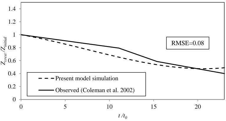
The proposed model of the breach crest height is compared against data from the work of Coleman et al. (2002) to test the model against similar cases. The experiments presented by Coleman et al. (2002) were originally conducted by Jack (1996) and Andrews (1998). This study is selected for the following reasons: 1) the availability of the input parameters required for the proposed model; 2) similarity of the grain sizes; and 3) use of

non-cohesive soil.

Using Eq. 3.3, variation of the maximum breach crest height with time was predicted for the case with medium sand (0.5 mm). The following parameters are used in the model: upstream reservoir length Lo = 11.16 m; initial water height in the upstream

reservoir ho = 0.3 m; initial height of the crest 𝑍𝑍_{𝑟𝑟𝑟𝑟𝑟𝑟𝑐𝑐𝑟𝑟𝑚𝑚𝑓𝑓} = 0.3 m; and non-dimensional dry

(41)

crest degraded mostly on a fixed upstream slope while the breach invert rotated around a pivot point. However, the pivot point in their study was along the base of the

embankment which prevented the embankment bottom length to advance farther

downstream. In the present study, the pivot point was located above the base and on the original downstream slope of the embankment, thereby allowing the advancement of the embankment bottom length with time. The proposed model (Eq. 3.3) is also used to estimate the final crest height for three small dam failures, i.e. Spring Lake Dam, Lower Rocky Ford Dam, and Upper Rocky Ford Dam, during the October 2015 flood in the Midlands area of South Carolina. The failure times for the above three cases are estimated by using USBR (1988) or Froehlich (1995). The comparison between the predicted and observed crest heights is in satisfactory agreement, as shown in Table 3.2 with RMSE equals to 0.28 m.

Moreover, the applicability of two selected models available in the literature, i.e. MacDonald and Monopolis (1984) and Singh and Scarlatos (1988), to predict the

experimental data presented in this study is examined. MacDonald and Monopolis (1984) studied 42 reported dam failure cases and developed two graphical relationships. The first one is relating the breach formation factor (BFF) which is the product of the outflow volume of water and the difference in elevation of the peak reservoir water surface and breach base plotted against the volume of the breach material removed, as shown in Figure 3.16 for earthen dams. The dashed line in the figure is the extension of their relationships since all their data were for field-scale dams. From the figure, it is seen that there is a small deviation between the experimental results and the fitted line. The

(42)

eroded material matches the recent cases of three small dam failures in South Carolina. The second relationship is relating the breach development time versus the volume of material removed during breaching. The relation for breach development time versus volume of eroded material proposed by MacDonald and Monopolis (1984) underpredicts breach time for both the experiments and the aforementioned field cases (Figure 3.17). Singh and Scarlatos (1988) developed analytical models for the analysis of

non-compacted gradual earth-dam failure. They used mass balance equation of reservoir, broad crested weir equation with the assumption of critical flow condition over the dam crest, and a breach-erosion equation. They applied the model to three breach shapes: rectangular, triangular, and trapezoidal. The comparison with the present work is only based on the rectangular breach shape to render the assumption of plane embankment erosion valid. The breach width is assumed to be equal to the entire width of the dam and the dam crest erodes vertically downward. According to the experimental data for the case with no-compaction, the relation between crest level (Zcrest) and time is non-linear

as shown in Figure 3.18. Therefore, non-linear erosion model of Singh and Scarlatos (1988) is applied. The input data for their model are as follows: Ho = 0.155 m, Zo = 0.15

m, 𝛼𝛼₁ = 1.5, As = 0.72 m2, b = 0.2 m. Singh and Scarlatos (1988) suggested a range of 𝛼𝛼₂

= 0.00015 to 0.0021 based on the comparison with historical data. When these values are tested with the present experimental data no agreement is found. Thus, four other

(43)

more gradual. As stated by Singh and Scarlatos (1988) the main drawback of their model is the value of 𝛼𝛼₂which is taken arbitrary and does not reflect any of the soil

(44)

Table 3.1 Test case characteristics

Test case Nb

(B/L)

𝛾𝛾𝑑𝑑

(kNm-3)

𝐶𝐶𝑒𝑒*

(kgcm-2)

1 0 13.35 0.00

2 10 14.75 0.91

3 20 15.46 1.82

4 30 15.47 2.72

* The compaction energy, 𝐶𝐶_𝑒𝑒, is defined as 𝐶𝐶_𝑒𝑒=(𝑁𝑁𝑏𝑏×𝑁𝑁𝑁𝑁𝑚𝑚𝑏𝑏𝑒𝑒𝑟𝑟𝑜𝑜𝑓𝑓𝑓𝑓𝑚𝑚𝑙𝑙𝑒𝑒𝑟𝑟𝑏𝑏×𝑅𝑅𝑚𝑚𝑚𝑚𝑚𝑚𝑒𝑒𝑟𝑟𝑤𝑤𝑒𝑒𝑟𝑟𝑟𝑟ℎ𝑐𝑐×𝑅𝑅𝑒𝑒𝑓𝑓𝑒𝑒𝑚𝑚𝑏𝑏𝑒𝑒ℎ𝑒𝑒𝑟𝑟𝑟𝑟ℎ𝑐𝑐)

𝑆𝑆𝑜𝑜𝑟𝑟𝑓𝑓𝑣𝑣𝑜𝑜𝑓𝑓𝑁𝑁𝑚𝑚𝑒𝑒𝑁𝑁𝑟𝑟𝑑𝑑𝑒𝑒𝑟𝑟𝑟𝑟𝑚𝑚𝑚𝑚𝑚𝑚𝑒𝑒𝑟𝑟

Table 3.2 Comparison between the predicted and observed crest heights for the SC floods

Lake area (m2₎

Breach width

(m)

Breach depth

(m)

Observed

Zcrest (m)

Predicted

Zcrest (m)

Spring Lake 192311 21.4 3.16 1.11 0.67

Lower Rocky Ford 102856 18 4.6 1.47 1.56

(45)

27

Figure 3.1 Schematic diagram of the experimental tests: (a) side view; (b) plan view (a)

(b)

Flow straightener

Dye container

Upstream edge of the

crest Dye container

Q

Camera

(46)

Figure 3.2 Repeatability of the progressive failure process for Nb = 10 blows/layer at: (a) t = 5 s;

(b) 10 s; (c) 15 s; (d) 25 s; (e) 40 s; and (f) 60 s

0 0.05 0.1 0.15

0 0.5 1 1.5

Be d E le v at io n ( m )

Distance from Upstream (m) Time = 10 s

0 0.05 0.1 0.15

0 0.5 1 1.5

0 0.05 0.1 0.15

0 0.5 1 1.5

0 0.05 0.1 0.15

0 0.5 1 1.5

0 0.05 0.1 0.15

0 0.5 1 1.5

Distance from Upstream (m) Time = 60 s 0

0.05 0.1 0.15

0 0.5 1 1.5

Exp. 1 Bed

Exp. 2 Bed Exp. 4 Bed

(47)

Figure 3.3 Breach evolution for different compaction efforts: Nb = 0 (a); Nb = 10 (b); Nb = 20 (c);

and Nb = 30 (d) 0.00 0.05 0.10 0.15

0.0 0.5 1.0 1.5

E le v at io n ( m )

Distance in x-direction (m)

Nb= 30 0.00

0.05 0.10 0.15

0.0 0.5 1.0 1.5

N_b= 20 0.00

0.05 0.10 0.15

0.0 0.5 1.0 1.5

Nb= 10 0.00

0.05 0.10 0.15

0.0 0.5 1.0 1.5

N_b= 0

t = 5 s t = 10 s t = 15 s t = 25 s t = 40 s t = 60 s

(48)

Figure 3.4 Degradation rate of the embankment crest for different compaction levels

Figure 3.5 Downstream hydrograph for different compaction efforts

0 0.0005 0.001 0.0015 0.002 0.0025 0.003 0.0035 0.004 0.0045 0.005

10 20 30 40 50 60

Dra

te

(m

/s

)

t(s)

No Compaction

10 B/L

20 B/L

30 B/L N_b= 0 N_b= 10

N_b= 20 Nb= 30

0.000 0.006 0.012 0.018

0 10 20 30 40 50 60 70 80 90

q

(m

3/s

/m

)

t(s)

Nb = 0

Nb = 10

Nb = 20

(49)

Figure 3.6 Correlation of normalized peak breach discharge and normalized dry density of the embankment

Figure 3.7 Correlation of normalized time to peak discharge and normalized dry density of the embankment

y = -12.80x + 17.42 R² = 0.93

0 1 2 3 4 5 6 7

0.84 0.86 0.88 0.9 0.92 0.94 0.96 0.98 1

qpe

ak

/qbas

e

α

y = 16.62x - 10.74 R² = 0.64

0 1 2 3 4 5 6 7 8

0.84 0.86 0.88 0.9 0.92 0.94 0.96 0.98 1

tpeak

/t0

(50)

Figure 3.8 Comparison between experimental and empirical results of the breach outflow hydrograph for: (a) Nb = 0; (b) Nb = 10; (c) Nb = 20; and (d) Nb = 30

0 1 2 3 4 5 6 7

0 5 10 15 20 25 30 35

q

/qbas

e

t/t₀

Experimental

Equations

RMSE = 0.24

(a)

0 1 2 3 4 5 6 7

0 5 10 15 20 25 30 35

q

/qbas

e

t/t₀

Experimental

Equations

RMSE = 0.28

(51)

Figure 3.8 (continued) Comparison between experimental and empirical results of the breach outflow hydrograph for: (a) Nb = 0; (b) Nb = 10; (c) Nb = 20; and (d) Nb = 30

0 1 2 3 4 5 6 7

0 5 10 15 20 25 30 35

q

/qbas

e

t/t₀

Experimental

Equations

RMSE = 0.42

(c)

0 1 2 3 4 5 6 7

0 5 10 15 20 25 30 35

q

/qbas

e

t/t₀

Experimental

Equations

RMSE = 0.30

(52)

Figure 3.9 Time variation of dimensionless embankment crest height for different compaction levels using Eq. 3.3

0.00 0.20 0.40 0.60 0.80 1.00

0 5 10 15 20

Zcr es t /Zin it ial t/t0 No compaction 10 B/L 20 B/L 30 B/L

N_b= 0 N_b= 10 N_b= 20 N_b= 30

0.00 0.20 0.40 0.60 0.80 1.00

0 5 10 15 20

Zcr es t /Z in it ial t/t₀ Experimental Equation (a)

N_b= 0

R2_{= 0.94}

0.00 0.20 0.40 0.60 0.80 1.00

0 5 10 15 20

Zcr es t /Z in it ial t/t0 Experimental Equation

N_b= 20

R2_{= 0.99}

(53)

Figure 3.11 Time variation of dimensionless embankment length for different compaction levels using Eq. 3.4

0.00 0.50 1.00 1.50 2.00 2.50

0 5 10 15 20

Lbase

/L

in

it

ial

t/to No compaction

10 B/L

20 B/L

30 B/L

(54)

Figure 3.12 Comparison between experimental and empirical results of temporal changes of normalized embankment bottom length for: (a) Nb = 10; and (b) Nb = 30

Figure 3.13 Schematic diagram of proposed triangular model to predict the progressive breach shape (image by author)

0.00 0.50 1.00 1.50 2.00 2.50

0 5 10 15 20

Lbase /Lin

it

ial

t/to Experimental

Equation

N_b= 10

R2_{= 0.94}

(a)

0.00 0.50 1.00 1.50 2.00 2.50

0 5 10 15 20

Lbase

/L

in

it

ial

t/t_o

Experimental

Equation

Nb= 30

R2_{= 0.97}

(55)

Figure 3.14 Measured and predicted bed surface profiles using the triangular model for Nb = 20

at: (a) t = 10 s; (b) t = 25 s; (c) t = 40 s; and (d) t = 60 s

0.00 0.05 0.10 0.15

0.0 0.2 0.4 0.6 0.8 1.0 1.2 1.4

z

(m)

t= 10 s Experiment

Equation

(a)

0.00 0.05 0.10 0.15

0.0 0.2 0.4 0.6 0.8 1.0 1.2 1.4

z

(m)

t= 25 s Experiment

Equation

(b)

0.00 0.05 0.10 0.15

0.0 0.2 0.4 0.6 0.8 1.0 1.2 1.4

z

(m)

t= 40 s Experiment

Equation

(c)

0.00 0.05 0.10 0.15

0.0 0.2 0.4 0.6 0.8 1.0 1.2 1.4

z

(m)

t= 60 s Experiment

Equation

(56)

Figure 3.15 Observed and predicted normalized crest height variation with time

Figure 3.16 Outflow Characteristics vs. eroded volume

0 0.2 0.4 0.6 0.8 1 1.2 1.4

0 5 10 15 20

Zcr

es

t

/Zinitia

l

t /t0 Present model simulation

Observed (Coleman et al. 2002)

RMSE=0.08

1E-05 1E-03 1E-01 1E+01 1E+03 1E+05 1E+07 1E+09 1E+11

1E-05 1E-03 1E-01 1E+01 1E+03 1E+05 1E+07

B

F

(m

3.m)

Volume of eroded material(m3₎

MacDonald and Monopolis (1984) Experimental

(57)

Figure 3.17 Breach development time vs. eroded volume

Figure 3.18 Time variation of dam crest level using the experimental data of no-compaction and the results of the mathematical model with different values of 𝛼𝛼₂

1E+00 1E+01 1E+02 1E+03 1E+04 1E+05

1E-03 1E-01 1E+01 1E+03 1E+05 1E+07

B rea ch in g tim e (s )

Volume of eroded material(m3₎

MacDonald and Monopolis (1984) Experimental

Spring Lake Lower Rocky Ford Upper Rocky Ford

0 0.02 0.04 0.06 0.08 0.1 0.12 0.14 0.16 0.18

0 10 20 30 40 50 60

Zcr

es

t

(m)

t(s)

Experimental (0 B/L)

Singh&Scarlatos 1988 (alpha 2=0.15) Singh&Scarlatos 1988 (alpha 2=0.20) Singh&Scarlatos 1988 (alpha 2=0.25) Singh&Scarlatos 1988 (alpha 2=0.3)

(α2=0.15)

(α₂=0.20) (α2=0.25)

(58)

CHAPTER 4 N

UMERICAL

M

ODELING OF

E

ARTHEN

D

AM

B

REACH DUE TO

O

VERTOPPING

:

I

NFLUENCE OF

D

IFFERENT

M

ODEL

P

ARAMETERS

In this chapter, the iRIC-Nays2D software, developed by Foundation of Hokkaido River Disaster Prevention Research Center for the calculation of unsteady 2D plane flow based on depth-averaged shallow water equations and morphology, is applied to a homogenous dam failure to study the influence of the different model parameters on dam failure prediction. Experiments on embankment failure by overtopping were conducted in a flume at the Hydraulics Laboratory, University of South Carolina. The model was run using different solution schemes, turbulence models, bedload formulas, and sediment transport mode (bed load only or bed load and suspended load). The Manning roughness coefficient and void ratio are selected by conducting a number of preliminary model runs.

4.1 Experimental Setup

(59)

The upstream toe of the embankment was considered to be the origin of the coordinate system. The embankment dimensions for all three tests were: embankment height = 0.15 m, embankment width = 0.2 m, embankment crest length = 0.1 m, upstream and

downstream embankment slopes (V: H) = 1:2.

4.2 Test Procedure

Prior to the embankment overtopping tests, Standard Proctor Compaction tests (ASTM D698) were carried out to determine the optimum water content of the homogenous, non-cohesive soil (i.e., sand only) used in the experiments. The optimum water content was found to be 5.2%. For each overtopping experiment, the soil was uniformly mixed with water to attain the optimum water content. To avoid compression, the soil was placed into three, 5 cm loose layers and no compaction was applied. For each layer, the soil surface was levelled precisely. After placing the third layer, the upstream and downstream faces of the embankment were trimmed carefully to reach the final trapezoidal shape. The seepage through the embankment was controlled and reduced by a thin clay layer with low permeability placed on the upstream face of the embankment.

(60)

negligible). The starting time of the failure process was considered to be the time when the water surface reached the front edge of the embankment crest.

Because of the limited width (i.e., 0.2 m), all three embankments were overtopped by the flow over the entire width resulting in a plane breach process (Pontillo et al. 2010, Schmocker and Hager 2009). So, the longitudinal embankment profile observed through the Plexiglas side of the flume represents the entire embankment. As indicated by Schmocker and Hager (2009), the sidewall effect was negligible. During the breach evolution, the water surface and bed surface profiles were recorded by an HD camera. By an image processing MATLAB code, the videos were converted into frames for one-second time intervals and then the longitudinal water and bed surface profiles were obtained by digitizing the frames.

4.3 Model Description

Numerical simulations were carried out using the iRIC software-Nays2D solver

(61)

In the following paragraphs, the basic flow and sediment transport equations in orthogonal coordinate system (x,y) are presented. To conserve space, the transformed forms of these equations into general coordinate system are not discussed here. The equations in general coordinate system are solved using the finite-difference method on the boundary-fitted structured grids. In addition, the software has a slope collapse model. If the angle of the bed exceeds a specified critical angle, the bed elevation is modified to satisfy the critical angle. The slope collapse model was not used in this investigation.

Following is the sequence of computations in the model: First, the 2D depth-averaged flow filed is calculated on the boundary-fitted structured grid using the finite-difference method based on the initial and boundary conditions Second, sediment

transport rate equations (i.e., bedload and suspended load) are calculated; finally, the bed deformation is determined using the 2D sediment continuity equation and bed elevation for all nodes is updated. An iterative process is applied to solve the equations for the unknown nodal values and these steps are repeated for a given time duration.

Flow Equations

The depth-averaged continuity equation for two-dimensional unsteady flow is:

𝜕𝜕ℎ 𝜕𝜕𝑡𝑡 +

𝜕𝜕(𝑢𝑢ℎ)

𝜕𝜕𝜕𝜕 +

𝜕𝜕(𝑣𝑣ℎ)

𝜕𝜕𝜕𝜕 = 0 (4.1)

in which t = time, h = water depth, x = streamwise coordinate, y = transverse coordinate,

u = velocity in the x direction, and v = velocity in the y direction.

The depth-averaged momentum equations in the x- and y- direction are

𝜕𝜕(𝑢𝑢ℎ)

𝜕𝜕𝑡𝑡 +

𝜕𝜕(ℎ𝑢𝑢2₎

𝜕𝜕𝜕𝜕 +

𝜕𝜕(ℎ𝑢𝑢𝑣𝑣)

𝜕𝜕𝜕𝜕 = −ℎ𝑔𝑔

𝜕𝜕ℎ 𝜕𝜕𝜕𝜕 −

𝜏𝜏𝑚𝑚

(62)

𝜕𝜕(𝑣𝑣ℎ)

𝜕𝜕𝑡𝑡 +

𝜕𝜕(ℎ𝑢𝑢𝑣𝑣)

𝜕𝜕𝜕𝜕 +

𝜕𝜕(ℎ𝑣𝑣2₎

𝜕𝜕𝜕𝜕 = −ℎ𝑔𝑔

𝜕𝜕ℎ 𝜕𝜕𝜕𝜕 −

𝜏𝜏𝑙𝑙

𝜌𝜌 +𝐷𝐷𝑙𝑙 (4.3)

where

𝜏𝜏𝑚𝑚

𝜌𝜌 = 𝐶𝐶𝑓𝑓𝑢𝑢�𝑢𝑢2+𝑣𝑣2 (4.4)

𝜏𝜏𝑙𝑙

𝜌𝜌 =𝐶𝐶𝑓𝑓𝑣𝑣�𝑢𝑢2+𝑣𝑣2 (4.5)

𝐷𝐷𝑚𝑚 ₌ 𝜕𝜕 𝜕𝜕𝜕𝜕 �𝑉𝑉𝑐𝑐 𝜕𝜕(𝑢𝑢ℎ) 𝜕𝜕𝜕𝜕 �+ 𝜕𝜕 𝜕𝜕𝜕𝜕 �𝑉𝑉𝑐𝑐 𝜕𝜕(𝑢𝑢ℎ)

𝜕𝜕𝜕𝜕 � (4.6)

𝐷𝐷𝑙𝑙 ₌ 𝜕𝜕 𝜕𝜕𝜕𝜕 �𝑉𝑉𝑐𝑐 𝜕𝜕(𝑣𝑣ℎ) 𝜕𝜕𝜕𝜕 �+ 𝜕𝜕 𝜕𝜕𝜕𝜕 �𝑉𝑉𝑐𝑐 𝜕𝜕(𝑣𝑣ℎ)

𝜕𝜕𝜕𝜕 � (4.7)

where g = gravitational acceleration, 𝜏𝜏_𝑚𝑚 = bed shear stress in the x direction, 𝜏𝜏_𝑙𝑙 = bed

shear stress in the y direction, 𝐶𝐶_𝑓𝑓 = bed shear coefficient, and 𝑉𝑉_𝑐𝑐 = eddy viscosity

coefficient. The 𝐷𝐷𝑚𝑚 and 𝐷𝐷𝑙𝑙 in the momentum equations are known as diffusion terms. Two available finite-difference methods in the model can be applied to the advection terms in the momentum equations: ‘the upwind difference method’ and the ‘CIP method’. The bed friction coefficient, 𝐶𝐶_𝑓𝑓, is estimated using Manning constant, 𝑛𝑛_𝑚𝑚, as follows

𝐶𝐶𝑓𝑓 =g𝑛𝑛𝑚𝑚 2

ℎ1/3 (4.8)

Sediment Transport and Bed Deformation Equations

In order to calculate the bedload transport rate by using either the A.M. formula or the M.P.M formula, the value of the dimensionless bed shear stress, 𝜏𝜏_∗, should be known. By applying Manning equation, 𝜏𝜏_∗ can be expressed as follows

𝜏𝜏∗ =_𝑠𝑠ℎ𝐼𝐼𝑒𝑒 𝑟𝑟𝑑𝑑 =

𝐶𝐶𝑓𝑓𝑉𝑉2 s𝑟𝑟𝑔𝑔𝑑𝑑 =

𝑛𝑛𝑚𝑚2𝑉𝑉2

(63)

bed material, and V is the composite velocity defined by the following equation

𝑉𝑉 =�𝑢𝑢2₊_𝑣𝑣2 (4.10)

A.M. formula for bedload transport rate, (1972)

The total bedload transport rate in the depth-averaged velocity direction (in the V

direction), 𝑞𝑞_𝑏𝑏, is given by

𝑞𝑞𝑏𝑏 = 17𝜏𝜏∗3/2�1−𝜏𝜏_𝜏𝜏∗𝑐𝑐

∗� �1− �

𝜏𝜏∗𝑐𝑐

𝜏𝜏∗� �s𝑟𝑟𝑔𝑔𝑑𝑑

3 _(4.11)

The dimensionless critical shear stress,𝜏𝜏_∗𝑐𝑐, is obtained from the Iwagaki’s equation (Iwagaki 1956).

M.P.M formula for bedload transport rate, (1948)

𝑞𝑞𝑏𝑏 = 8(𝜏𝜏∗− 𝜏𝜏∗𝑐𝑐)1.5�s𝑟𝑟𝑔𝑔𝑑𝑑3 (4.12)

Two-dimensional continuity equation of sediment transport, Exner equation

𝜕𝜕𝜕𝜕 𝜕𝜕𝑡𝑡 +

1 1− 𝜆𝜆 �

𝜕𝜕𝑞𝑞_𝑏𝑏𝑚𝑚

𝜕𝜕𝜕𝜕 + 𝜕𝜕𝑞𝑞_𝑏𝑏𝑙𝑙

𝜕𝜕𝜕𝜕 +𝑞𝑞𝑏𝑏𝑁𝑁− 𝑤𝑤𝑓𝑓𝑐𝑐𝑏𝑏�= 0 (4.13)

in which 𝜕𝜕 = bed elevation, 𝑞𝑞_𝑏𝑏𝑚𝑚 and 𝑞𝑞_𝑏𝑏𝑙𝑙 = bed load transport rate per unit width in the x

and y directions, respectively, 𝑞𝑞_{𝑏𝑏𝑁𝑁} = suspended load supplied per unit area of bed and is calculated based on the equation proposed by Itakura and Kishi (1980), 𝑤𝑤_𝑓𝑓 = settling

velocity of suspended sediment which is obtained with Rubey’s equation (Rubey 1933),

𝑐𝑐𝑏𝑏 = concentration at the control point (i.e., near the bottom), and 𝜆𝜆= void ratio of bed