ABSTRACT
CHENG, YIJING. Underfunding of State and Local Pension Plans in the United States: The Role of the Dependency Ratio. (Under the direction of Lee Craig).
The underfunding of public sector pension plans in the United States is a potentially serious problem. According to analysis conducted by the Pew Center, as of 2008, there was a $1 trillion funding gap between the $2.35 trillion states and participating localities ha ve set aside to pay for employees‘ retirement benefits and the $3.35 trillion value of their pension liabilities. Many observers have noted that the cause of the funding gap is the poor performance of the U.S. stock market since 2007. This performance reduced the returns on the assets in the pension fund portfolios and thus exacerbated the funding gap. However, my thesis focuses on another important factor—the dependency ratio, which is the ratio of pension fund beneficiaries to workers. Specifically, I focus on how the dependency ratio affects the funding ratio.
Underfunding of State and Local Pension Plans in the United States: The Role of the Dependency Ratio
by Yijing Cheng
A thesis submitted to the Graduate Faculty of North Carolina State University
in partial fulfillment of the requirements for the degree of
Master of Arts
Economics
Raleigh, North Carolina 2011
APPROVED BY:
_______________________________ ______________________________ Lee Craig Robert Clark
Committee Chair
DEDICATION
致父母
谢谢你们一直在我身后支持我,鼓励我
BIOGRAPHY
ACKNOWLEDGMENTS
I want to express my deepest and most sincere gratitude to Professor Lee Craig. From the very beginning of this thesis, he helped me learn the background of the research field, and motivated me to do the analysis so as to successfully complete my thesis. He has been so patient to explain all kinds of questions I had during the research and analysis. Furthermore, he edited the draft of my thesis so carefully and made it the way it is now.
I also want to convey my appreciation to Professor Robert Clark from the Department of Economics and Professor Wenbin Lu from the Department of Statistics who are the other committee members who helped me with some questions regarding my thesis. In additio n, I would like to thank Dr. Tamah Morant and Ms. Robin Carpenter, who offered me a lot of important information and helped with my two-year study and the graduation application as well.
TABLE OF CONTENTS
LIST OF TABLES………..vi
LIST OF FIGURES………vii
Issues………1
Model………...6
Data………15
Results………19
Conclusions………25
Tables……….30
Figures………....37
LIST OF TABLES
Table 1 Employee Contribution Rates in 2006 and 2008………...30 Table 2 Descriptive Statistics: Means and Standard Deviations of the Data………..31 Table 3 Linear Model of Funding Ratio with Dependency Ratio………...32 Table 4 Linear Model of Funding Ratio with Dependency Ratio
and Benefit Value………...33 Table 5 Linear Model of Funding Ratio with Dependency Ratio
Benefit Value and Employee Contribution………....34 Table 6 State and Local Pension Plans, Which Have Large Dependency Ratios…...35 Table 7 The Number of Beneficiaries and Workers for the Pension Plans having a
Larger Dependency Ratio in 2008 than in 1990……….36
LIST OF FIGURES
Issues
By the end of the twentieth century, defined benefit retirement plans remained
the major type of pension plans in the public sector in the United States ; whereas in
the private sector, defined contribution plans are the most prominent type of plan
(Clark et al 2011, p. 159-160). With a defined benefit pension, public sector
employees, such as those who work for states and municipalities, promise
workers--including teachers, firefighters and policemen--a specified benefit at retirement. The
benefit is predetermined by a formula, typically based on three things: the employee ‘s
earning history, years of service, and a multiplier or ―generosity factor‖. So if all goes
well, when the employees retire, they will receive the promised benefits from their
employers. But what happens if the public employers face some type of financial
crisis? Will the employees actually receive the full value of the promises they have
received at or beyond the time of retirement?
An analysis by the Pew Center on the States1 states that ―at the end of fiscal year
2008, there was a $1 trillion gap between the $2.35 trillion the states and participating
localities had set aside to pay for their employees‘ retirement benefits and the $3.35
1
trillion price tag of those promises‖ (Pew Center, 2010, p.1). To be specific, in the
fiscal year 2008, public employers have promised employees $3.35 in future benefits,
but those employers can only have $2.35 in assets to make those payments. Thus there
is a $1 trillion gap between these two figures, which means the retirees may not get
fully paid as promised; or public employers, which means taxpayers, will have to
increase their contributions to the plans; or current employees will have to increase
their contributions; or some combination of these will be required to balance the plans‘
liabilities and assets. (Other estimates, using a different rate to discount future
liabilities, place the gap as high as $2.5 trillion. See Rauh and Novy-Marx, 2011.)
Furthermore, Pew‘s figure is arguably conservative because it onl y calculates
total assets in the public sector plans to the end of fiscal year 2008, which usually
ends on June 30, 2008. So the downturn of the pension fund investments , which were
subsequently affected by the worse economic environment in the second half year of
2008 were not shown in the figure. Another reason is that ―most states‘ retirement
systems allow for the ‗smoothing‘ of gains and losses over time‖ (Pew Center, 2010,
p. 1), which means that the effect of the losses in the investment returns will continue
to erode the balance sheets of the public sector pension plans over the next couple of
years. Because of these two reasons, the funding gap from Pew‘s analysis might be
This funding gap creates a potential crisis in the state‘s pension systems, whic h
may cause many other problems. For example, employees may become dissatisfied
with the states‘ systems, and fewer people will be attracted to work for public sector
employers. Or if taxpayers are called upon to ―bail out‖ the plans, the upward pressure
on tax rates would create a deadweight loss and might discourage real economic
activity, which would shrink the tax base and put even more upward pressure on tax
rates, creating a potentially harmful spiral.
It is worth considering how the nation‘s state and local pension plans got in so
much trouble. Pew‘s analysis also compared the current situation with that in 2000.
There was no big shortfall in pension funding at the beginning of the twenty-first
century; the problem began more recently. ―In 2000, state-run pension plans were
actually running a $56 billion surplus. From 2000 to 2008, growth in pension
liabilities had outstripped growth in assets by more than $500 billion. In 2000, more
than half the states were fully funded. By 2006, that number had shrunk to six states.
By 2008, only Florida, New York, Washington and Wisconsin could make that claim‖
(Pew Center, 2010, p.16).
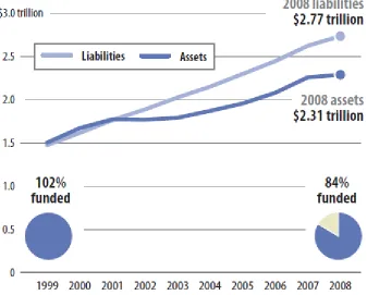
From Figure 1, we can see that in 1999 and 2000, the funding was quite strong,
in that pension plans were 102% funde d on average, which means that the assets
could fully cover the liabilities in those years, and the public sector employees could
follow the increase in liabilities. In fiscal year 2008, the state systems were 84 percent
funded in the aggregate. In other words, the assets could only cover 84 percent of the
total liabilities, which yields the gap between assets and liabilities, which is the $1
trillion mentioned earlier.
Figure 1
According to the National Bureau of Economic Research, the recent recession
began in December 2007. And it also affected the stock market severely. ―In calendar
year 2008, public sector pension plans experienced a median 25 perce nt decline in
their investments‖ (Pew Center, 2010, p. 5). Therefore, many analysts and scholars
argue that the $1 trillion gap between assets and liabilities was caused by the
recession. Is this true? Partly. Refer back to Figure 1. Note that the gap between
liabilities and assets from 2001 to 2007 is increasing all the time. So even before the
recession, the state pension systems were underfunded, and had been for several years.
In this case, the recession in 2007 might be a reason for making the funding situation
worse; and it might be the most dominant reason why the gap is increasing; but it is
not the only reason.
There is other evidence which shows that the economic recession is not the only
this bill coming due. States such as Florida, Idaho, New York, North Carolina and
Wisconsin all entered the current recession with fully funded pensions . But many
other states are struggling. At the end of fiscal year 2008, 21 states had funding levels
below the 80 percent mark, compared with 19 below that level in 2006‖ (Pew Center,
2010, p.17). The influence of the recession and the stock market is nationwide, but the
performance of the states is quite different. In this thesis, I argue that there is at least
one other major factor at work, one that differs state to state; one that affects the
different performance of the states. In other words, the funding ratio might have a
relationship with some other factors, which can be identified among different states.
One of these which I look at is the ―dependency ratio‖, which is the ratio of the
number of dependents of a pension plan to its current contributors. In other words it is
the ratio of retirees (who receive a pension) to employees (who contribute to the
Model
The funding ratio provides valuable information about the actuarial soundness of
a pension fund, and is thus of much interest to us. In the model that follows I propose
to explain the behavior of the funding ratio in state-managed pension funds in the
United States. Recall that the funding ratio is the ratio of assets held by the pension
fund to the present value of fund liabilities – that is the promises to the employees. If
a state ‘s system is fully funded, then the funding ratio is 1 or greater than 1. In general,
the larger the funding ratio, the better funded is the state ‘s pension plan. I‘m interested
in how the funding ratio is related to other factors. Henceforth, I refer to the funding
ratio as ―FRATIO‖.
A variable that plays a role in explaining the behavior of the funding ratio is the
dependency ratio, which, again, is the ratio of beneficiaries to workers – i.e. ―it is the
number of retirees dependent on benefits relative to the number of workers supporting
them‖ (Scheiber and Shoven, 1999, p.72). If the dependency ratio is 1, it means that
for every retiree receiving a pension from a particular fund, there is one employee
contributing to the fund. Of course this scenario is unlikely to happen in real world.
Conversely, if the dependency ratio is zero, there are no retirees receiving a benefit
from the fund. The larger the dependency ratio, the larger is the number of retirees per
To see the relationship between the dependency ratio and the funding ratio,
consider the simple ―pay-as-you-go‖ retirement system, in which the total benefits
paid to the employees every year, which are expenditures for the pension system,
have to be equal to the total contributions collected. In other words, ―The amount of
benefits paid is equal to the total number of people getting benefits times the average
benefit paid by the system‖ (Scheiber and Shoven, 1999, p.72). The amount of
contributions, from workers and employers, available to the system is equal to the
contribution rate, including both the employer and employee portion of the
contribution, times the number of workers who contribute to the fund, times workers‘
average earnings.
Although most public sector retirement plans in the United States do not operate
on a pay-as-you-go basis, the basic model will help set up the connection between the
dependency ratio and the funding ratio. The math of such a system is shown in
equation [1] below. The required contribute rate to support such a system is the
product of the relative number of beneficiaries and wor kers times the ratio of average
benefits to average covered earnings, which is shown in equation [2].
The Mathematical Operations of an ideal Retirement Plan
Contributions = Expenditures
where:
c = contribution rate paid by employers and employees
NW = number of covered workers employed in a year
W = average wages of workers during the year
NB = number of retirees receiving benefits
B = average benefits paid to retirees
and such that:
[2] c = (NB / NW) · (B / W)
So the dependency ratio in this simple model is the ratio of beneficiaries to
workers (NB / NW); while (B / W) is the ratio of average benefits to average wages in
a retirement, which is often referred to as the ―replacement rate‖ – ―it reflects how
much of an average worker‘s earnings are replaced by the retirement benefit when he
or she retires‖ (Sylvester, 1999, p.72). As a result, the contribution rate equals the
product of the dependency ratio and the replacement rate.
Equation [2] shows that if the dependency ratio increases, then either the
contribution rate must increase, or the replacement rate must decrease. In the United
States, on average, for many public sector pension plans, the replacement rate has
increased over time. ―In 1982 the mean replacement rate for teachers was 53.0 percent.
(that is, roughly 10 percent) to 58.5 percent‖ (Clark et al., 2011, p. 88). So we can see
that if the replacement rate has been increasing, then either the contribution rate will
increase or the dependency ratio must decrease.
Of course, this model is a simplification. The creation of a pension fund
complicates matters, because the funding strategy of the employer might be very
complex. In what follows it might be best to think of the changes in the funding ratio
as a response to unanticipated changes in the dependency ratio, since presumably
anticipated changes would have already been a part of the employer‘s funding
strategy2.
We now connect this relationship to the funding ratios of the state -managed
plans. Recall that the funding ratio is the ratio of assets to the present value of
liabilities. The denominator is a function of the dependency ratio, in that if the
dependency ratio goes up (i.e. there are more beneficiaries given the same number of
workers), holding other variables constant, then the system has to pay more to the
retirees and the present value of liabilities increases. So if the value of fund assets
stays the same, the funding ratio will decrease as the dependency ratio increases.
But the assets in the numerator are mathematically linked with worker and
employer contributions. At any point in time the current assets are a function of past
contributions and earnings from the fund.
2
[3] Assett = (ρ t-1 * Assetst-1) + Assett-1 + Contributionst-1 – Distributionst-1
Like in Equation [3], the amount of assets in tth period is the summary of the
investment returns of the (t-1)th period, the amount of the assets in the (t-1)th period,
the contributions of employers and employees in the (t-1)th period, and then minus
the distributions in (t-1)th period – that is the payments from the fund to retirees.
Specifically, ρ t-1 is the rate of investment returns in the (t-1)th period, so (ρ t-1 *
Assetst-1) is the increased investment from the asset in (t-1)th period. And the
distributions include the money paid to the retirees and other management and
administrative costs.
So if employers and employees contribute more to the fund, ceteris paribus, the
system has more assets, and from equation [2] above we already know that the
contribution rate will increase as the dependency ratio increases, holding the
replacement rate constant. (And since we know the replacement rate has on averaged
increased over time, this puts further upward pressure on the contribution rate.) So
holding earnings on the fund‘s assets constant, the numerator of the funding ratio
should increase as the dependency ratio increases, through higher contribution rates.
However, if contribution rates do not increase enough to offset the increase in the
constant. Consequently, we now see how the funding ratio is related to the
dependency ratio. What we now need is to estimate the size of this relationship.
Henceforth, I will use the name ―DEPRATIO‖ to represent dependency ratio.
Then I will build a linear model using FRATIO and DEPRATIO as the depe ndent and
independent variables, respectively.
[4] FRATIOit= α +β 1 DEPPRATIOit+ eit
Specifically, FRATIOit is the funding ratio of the ith state in tth year in the
United States; DEPRATIOit is the dependency ratio of the ith state in tth year; and eit
is the error of the model for every i and t, and eit has a mean of zero and a finite
variance. As for the coefficients, α is the intercept of the model, andβ 1 is the
coefficient of the variable DEPRATIO, i.e. it tells us the size of the rel ationship
between the dependency ratio and the funding ratio. If we cannot reject the hypothesis
that β 1 =0, it means that FRATIOit has no relationship with DEPPRATIOit . In other
words, such a result would lead me to conclude that the funding ratio for the state
pension plans in my sample has no linear relationship with dependency ratio. If
however β 1 >0, the n the funding ratio has a positive relationship with dependency
ratio, which means that if the dependency ratio increases, the funding ratio will also
however β 1 <0, the funding ratio will decrease as dependency ratio incre ases, the
finding suggested by our model above. So from this model, we can see how the
funding ratio changes as dependency ratio changes.
Considering that there are some other factors – other than the stock market, of
course – which may also influence the funding ratio, I will add some other variables
in model shown in equation [4]. The first other variable I will add is ―BenefitValue‖,
which is the formula multiplier or generosity factor in the pension plan. Since the
formula multiplier determines the pension annuity payment an employee will receive
from their employer, it will affect the denominator of funding ratio, ceteris paribus. So
my hypothesis is ―BenefitValue ‖ also has a relationship with ―FRATIO‖.
The multipliers vary from plan to plan. ―There are a wide range of formula
multipliers in effect for these 70 plans [the plans in the Wisconsin sample that are ―coordinated‖ with Social Security], which sometimes vary by number of years of
service, by date of employment, or by age at retirement. For 2008, the average
formula multiplier for the coordinated plans that are not money purchase plans,
defined contribution plans, or plans in which the employer determines the formula
multiplier is approximately 1.94%‖ (Schmidt, 2009, p. 26). In 2002, the average
formula multiplier was 1.99%. BenefitValueit is the formula multiplier of the ith state
[5] FRATIOit= α + β 1 DEPPRATIOit + β 2 BenefitValueit + eit
Running this model will yield the estimates of α , β 1 andβ 2. The explanation of
α and β 1 is the same as in the first model as shown in equation [4]. As for β 2, if it is
positive, it means that as the formula multiplier increases, funding ratio will also
increase. If, however, β 2 is negative, it shows that funding ratio has a negative
relationship with the formula multiplier. Because an increase in the multiplier will
increase pension liabilities, ceteris paribus, my hypothesis is that β 2 is negative.
Besides the signs of β 1 andβ 2, I will also see whether they are statistically
significant in this model, that is I want to test the hypotheses: β 1 = 0 andβ 2 = 0. If β 1 is statistically significant in this model, it means that the dependency ratio has a
statistically significant influence on the funding ratio. In addition, I am interested in
the size of the impact of the left-hand side variables on the funding ratio.
As our simple model above suggests, another important factor which may
influence funding ratio is employee contribution rates. ―Most public employee
pension plans at least nominally require employees to contribute a certain percentage
of their salary to the plan, although some public employee pension plans provide for
employer ‗pick-up‘ of the employee contribution‖ (Schmidt, 2009, p.19). So the
employee contribution rate is shown as a percentage of salary, or it is the ratio of the
salary. As Clark et al. note, ―We also analyzed employee contribution rates, which
vary from a low of zero – in Florida, Tennessee and Utah – to a high of 11.0 percent
in Massachusetts. Between 1984 and 2006, 22 states increased employee
contributions while nine states reduced the employee contributions rate‖ (Clark et al.,
2011, p. 96). Also, ―It appears most of the increase in employee contribution rates
occurred before 2002, as Brainard (2007), using a survey of plan administrators,
reports, as the mean employee contribution rates remained stable between 2002 and
2006. The employee contribution rate for states with Social Security coverage was 5.0
percent during this later period and the contribution rates for employees that were not
part of Social Security was 8.0 percent‖ (Clark et al., 2011, p.112).
The column in [Table 1] entitled ―Employee Contribution‖ shows the employee
contribution rates, expressed as a percentage of payrolls, for the 85 state-managed
plans covered in the report of Wisconsin Legislative Council in 2008.
So in the new model, there are now three independent variables: dependency
ratio, formula multiplier and employee contribution rates.
[6] FRATIOit=α + β 1 DEPPRATIOit+ β 2 BenefitValueit + β 3 EmployeeContit +
eit
In the next section I discuss the data used to run the three models, and in section
four I will present the results, focusing on the sign, statistical significance, and size of
Data
In this thesis, I employ data on the ―major‖ state-managed public employee
retirement systems in the United States. These data are from 85 of pension plans that
cover teachers, other state employees, and in some cases local employees as well. By ―major‖ plans, I mean the largest plans. Although there are more 2,500 state and local
pension plans in the United States (219 of which are state-managed), the 85 plans in
my sample represent the vast majority of state workers as well as the majority of local
workers. For example, Clark et al. note that 60 percent of local workers covered by a
plan are covered in the state-managed plans in the Wisconsin Legislative Council data.
The data are from the Wisconsin Legislative Council3, from 1990 to 2008 and they
are reported every other year (except 1998).
There are 85 plans in 9 years from 1990 to 2008 in the original data, which gives
me 765 observations. Then I deleted the observations with missing values of
employee contribution or benefit value (i.e. generosity parameter), so one or more
pension plans in the following states are missing data for one or more years: Arkansas,
3
California, Delaware, Florida, Georgia, Hawaii, Iowa, Kentucky, Maryland,
Massachusetts, Michigan, Mississippi, Missouri, Nebraska, Nevada, New Hampshire,
New Jersey, New Mexico, Oklahoma, Rhode Island, Tennessee, Texas, Utah,
Vermont, and Wisconsin. Finally, following this process, I ended up with 402
observations in my sample, and I sorted the final data by year and state.
From the original data, which provided much information on the state-managed
pension plans, I am interested in the following: Year, State, FundName,
EmployeeCov (i.e. what kind of employee does the plan cover); SSCoverage (if social
security is covered in the plan, then this variable equals 1; otherwise it is 0);
EmployeeCont (Employee Contribution rate, from 0 to 1); BenefitValue (formula
multiplier in a pension fund); FundRatio (i.e. the ratio of assets to the present value of
liabilities, displayed in percent); and the DepRatio (dependency ratio). Then I add a
new variable ―New_Fundratio‖, which displays FundRatio as a percentage – i.e. 95
rather than 0.95. I also created a set of dummy variables Dum1990, Dum 1992 ……
Dum2008, which represent the years.
To get a general idea of what the data look like, I generated descriptive statistics
for the variables. See [Table 2]. The data in [Table 2] show that the average funding
ratio in 2008 (0.796) is far less than the overall pool average from 1990 to 2008
(0.888), which means the underfunded situation has gotten more serious in recent
1990 to 0.532 in 2008. This change is driven by the much faster increase in retirees
than workers. (See Table 7, below.)
[Table 2]
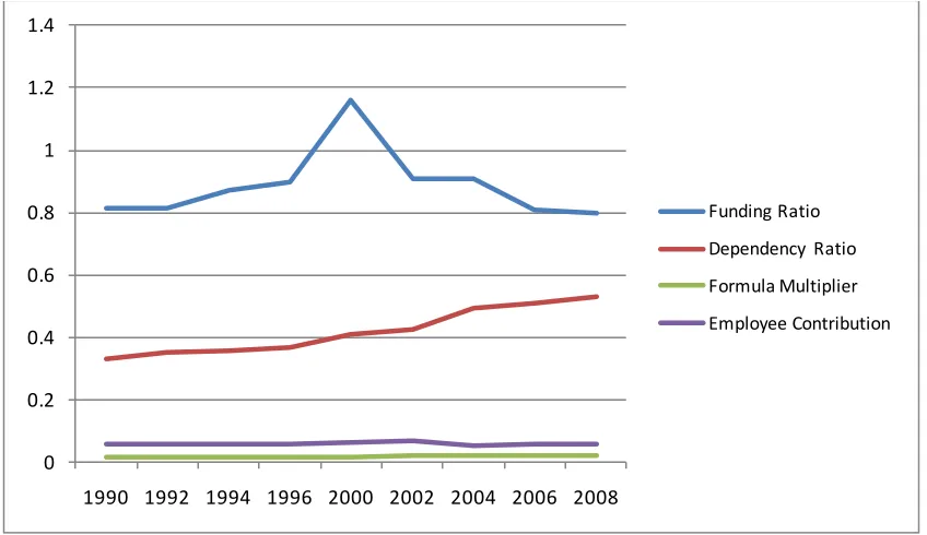
I also generated a figure to show how the mean values of these variables
developed from 1990 to 2008. In Figure 2, from the top to the bottom, they display
the development of the funding ratio, dependency ratio, formula multiplier and
employee contribution rate from 1990 to 2008, in the state-managed plans of my
sample.
With respect to the funding ratio, the figure shows a rapid increase from about
1997 to 2002, as the stock market performed well during that time. ―Defying skeptics
and historical precedent, the U.S. stock market soared again in 1997, allowing the
Dow Jones industrial average to post a gain of more than 20 percent for the third
consecutive year. It was a feat never before accomplished ‖ (Myers, February 1998, p.
21). And recall Equation [3] in Section 2, because the rate of investment returns is
high due to the soaring stock market during that time, the value of the assets in the
pension fund is also large. Therefore, the funding ratio increases rapidly after 1997.
Then it reached the peak in 2000, and faced a deep downturn after that. From
2002, the NASDAQ dropped to as low as 1,108.49 – a 78.4 percent decline from its
all-time high of 5,132.52, the level it had established in March 2000. The ups and
downs of the stock market clearly affected the funding ratio.
Now let us look at the most independent variable in our model – the dependency
ratio. It increases all the time, and in 1996, the increasing rate got a bit higher than ti
had been and even higher in 2002, until 2004.
As for the other two variables, the employee contribution bounced twice and
came back to the same level as in 1990. The mean formula multiplier remained almost
roughly constant from 1990 to 2008.
Results
A reminder: for convenience of interpretation, I express the funding ratio in
percentage terms and refer to it as ―New_Fundratio‖. In addition, I have added the
dummy variables to the base model, as reported in equation [4]; so the model I
actually estimate is:
[7] New_Fundratioit = α +β 1 DEPPRATIOit + γ 1 Dum1990 + γ 2 Dum1992 +γ 3
Dum1994 +γ 4 Dum1996 +γ 5 Dum2000 +γ 6 Dum2002 +γ 7 Dum2004 +γ 8
Dum2006 + eit
The results from estimating model (7) are shown in [Table 3]. The estimated
value of β 1 – i.e. the impact of the dependency ratio on the funding ratio is -0.45567
(0.18767). (Standard errors are in parentheses.) In other words, if in ith state in tth
year the dependency ratio increases by ten percentage points, which is less than one
standard deviation from the mean (from [Table 3]), the funding ratio will decrease by
4.5 percentage points. I would argue that, i n addition to being statistically significant,
the finding is economically significant, perhaps the equivalent of one year of liability
To explain the negative sign of β 1, I argue that if there are more retirees given
the same number of workers, i.e. if the dependency ratio increases, then the
underfunded situation will get worse. To see this, refer back to Section 2; the
dependency ratio equals beneficiaries divided by current employees, and the funding
ratio equals assets divided by liabilities. Thus, if beneficiaries increase relative to
employees (who make contributions to the fund, which increases assets), then, ceteris
paribus, there will be fewer contributions to assets in the numerator of the funding
ratio, relatively speaking of course, and more liabilities in the denominator.
As noted in Section 3, the dependency ratio has been increasing; so the present
value of liabilities is also increasing. And the amount of assets increases as the
contribution increases, again, ceteris paribus, which has a positive impact on the
funding ratio. But the funding ratio has been decreasing; so it follows that
contributions have not increased enough to keep up with the decrease in assets from
other causes (for example, the general decline in the value of financial assets during
the recent recession). (Clark et al. agree with this point (2011, p. 112)). Thus asset
values have fallen as liabilities have increased. In short, increases in contribution rates
cannot keep up with increases in retirees, holding other variables constant.
The t value of the estimated β 1 is -2.43, and the probability of the value that is
greater than the absolute value of t is 0.0156, which is smaller than 5 percent. So I can
reject the null hypothesis that the value of β 1 is zero, at the 5 percent level. Literally,
the dependency ratio can negatively affect the funding ratio in both economically and
statistically significant ways, regardless of what is happening in the stock market!
Now let us add another variable, BenifitValue, to model (4), which yields model
(5):
[8] New_Fundratioit = α +β 1 DEPPRATIOit +β 2 BenifitValue +γ 1 Dum1990 +
γ 2 Dum1992 +γ 3 Dum1994 +γ 4 Dum1996 +γ 5 Dum2000 +γ 6 Dum2002 +γ 7
Dum2004 +γ 8 Dum2006 + eit
From [Table 4], I get the estimated value of β 1 as -0.44472 (0.18888), which in
absolute value is a little smaller than the one in the model as expressed in equation [7].
In other words, if in the ith state in the tth year the dependency ratio increases by ten
percentage points, which, again, is less than one standard deviation from the mean,
and then the funding ratio will decrease by 4.4 percentage points. Again, I argue that
this result is statistically and economically significant. The t value of the estimated β
0.0190, which is smaller than 5 percent. So, again I conclude that the estimated value
of β 1 is statistically significant on the 5 percent level.
[Table 4]
As for the coefficient of ―BenefitValue‖ – i.e. the generosity parameter of benefit
multiplier in the defined benefit pension plan – β 2; in the model, the estimated
value is -4.09132 (7.39979). So, keeping the dependency ratio constant, if the
formula multiplier increases for 0.1, which would be a rather large increase (see
[Table 4]) the funding ratio will decrease 0.409132, which, would seem to be an
economically significant amount, though considerably smaller than the impact of
the dependency ratio. However, the t value is only 0.55, and the probability of
obtaining a value that is greater than the absolute value of t is 0.5806 , which is
much greater than 10 percent. So the estimated value of β 2 is not statistically
significant – that is to say, I cannot reject the hypothesis that β 2 is zero. In any case,
it is worth discussing the negative sign of β 2. It says, in essence, if the formula
multiplier increases, then employers will promise to pay more to the beneficiaries,
which will increase the present value of liabilities. So the funding ratio will
Now let‘s add the third variable Employee Contribution Rate (EmployeeCont)
and build model (6), as shown in equation [9]:
[9] New_Fundratioit = α +β 1 DEPPRATIOit +β 2 BenifitValue +β 3 EmployeeCont
+γ 1 Dum1990 + γ 2 Dum1992 +γ 3 Dum1994 +γ 4 Dum1996 +γ 5 Dum2000 +
γ 6 Dum2002 +γ 7 Dum2004 +γ 8 Dum2006 + eit
From the results in [Table 5], I obtained an estimated value of β 1 as -0.44475
(0.18912), which is almost the same as found in the earlier estimates. So the
discussion is similar. Besides, the estimated value of the coefficient of Employee
Contribution is 0.00542 (0.06221). This means that, keeping the dependency ratio and
formula multiplier unchanged, if the employee contribution increases by 10
percentage points, the funding ratio will increase 0.000542. This would seem to be a
rather low number, and hence I conclude the impact of this variable is not
economically significant. Furthermore, t he probability of the value that is greater than
the absolute value of t is 0.9307, which is much greater than 10 percent. So, like the
benefit multiplier, it is not statistically significant.
From all the results above, I can conclude that the estimated value of β 1 is
between -0.44 and -0.46, which means that no matter whether the formula multiplier
and employee contribution affect the funding ratio or not, the estimated value of the
coefficient of dependency value is in the neighborhood of -0.45, and it is consistently
statistically significant. This result provides evidence to support the arguments I made
earlier in this thesis; that is, specifically, besides the huge investment losses resulting
from the large economic recession in the last a few years, the decreasing funding ratio
in the last 10 years has been at least partly driven by the increasing dependency ratio4.
Since many observers and scholars focus on the poor performance of the stock market
of recent years, my work suggests that we should transfer our attention to another
component of the reason that the state-managed pension plans are underfunded. From
the results of this thesis, I conclude the increasing dependency r atio is also an
important cause of the huge funding gap.
4
Conclusions
Scholars and others studying the recent ―crisis‖ in the funding of state and local
pension plans in the United States have focused on the performance of the stock
market since 2007. In contrast, this thesis analyzes the relationship between the
funding ratio (i.e. the ratio of pension plan assets to liabilities) of state -managed
pension plans and dependency ratio (i.e. the ratio of plan beneficiaries to workers).
Using the data on the major public employee retirement systems, which are provided
by Wisconsin Legislative Council from 1990 to 2008, I show that one of the key
reasons many state-managed retirement systems are currently so underfunded is
because of the movement in the dependency ratio, which worsened the funding status
of the plans in my sample.
As noted in section 1, there is currently a funding gap in state managed pension
plans. Estimates of the size of this gap range from $500 billion to several trillion
dollars, which means that the underfunded situation in the major public employee
retirement systems is really severe. From the data I employed in this study, the mean
funding ratio in 2008 was 0.796; while the mean ratio between 1990 and 2008 was
0.888. Thus roughly 20 percent of the aggregate pension liabilities of the
state-managed pension funds could not currently be paid to the retirees. ―Between the start
budget gap of $304 billion, according to the National Conference of State Legislatures
(NCSL). And revenues are expected to continue to drop still more during the next two
years. Under these conditions, many states have been and will continue to be forced to
make difficult decisions about where to invest their limited resources‖ (Pew Center,
2010, p. 22-23).
Since the onset of the recent recession, the stock market has declined
substantially. The Dow Jones Industrial Average closed at 14,164 on October 9, 2007
and has not come close since. It bottomed out below 6,600 in March 2009, a peak to
trough decline of more than 53 percent and currently remains around 12,000. So the
investment returns of the retirement systems have been decreasing, which to some
extent causes the value of assets to diverge from the present value of liabilities,
holding other factors constant. As noted, many people have already noticed and
studied the impact of the stock market. (Clark et al. show the importance of stock
market investments in the portfolios of public sector pension funds (2011, pp.
180-194).) However, this is not the only factor influencing the funding ratio. Instead, I‘m
looking at the relationship between dependency ratio and funding ratio.
Since the funding ratio is the ratio of assets in the fund to the present value of
liabilities, and as described in section 2, an increase in the dependency ratio will tend
to worsen the funding ratio, ceteris paribus, by increasing the present value of
ratio, an increase in retirees, ceteris paribus, increases the ratio and decreases the
funding ratio; whereas an increase in workers, again ceteris paribus, decreases the
dependency ratio but increases the funding ratio through increased contributions. As
we cannot determine unambiguously how the funding ratio changes as the
dependency ratio changes, I chose to employ econometrics to analyze the impact of
the dependency ratio on the funding ratio, controlling for other factors.
From section 4, we see that in the linear regression models the coefficient on the
dependency ratio is between -0.44 and -0.46, which suggests: (1) that funding ratio
has a negative linear relationship with the dependency ratio, and (2) that for every ten
percentage point increase in the dependency ratio, there is a roughly 4.5 percent
decrease in the funding ratio. Thus I argue the impact of an increasing dependency
ratio is both statistically and economically significant. As a result, I conclude the
increasing dependency ratio is an important factor that negatively affect s funding ratio.
As the dependency ratio is the number of beneficiaries relative to the number of
workers, there are four ways in which the dependency ratio can increase. One is an
increase in the number of beneficiaries (retirees); another is a decrease in the number
of workers. A third is an increase in both variables with the number of beneficiaries
increasing more than the number of workers; and the fourth is a decrease in both
beneficiaries. Of course, if the number of beneficiaries increases and the number of
workers decreases, then the dependency ratio will increase even more rapidly.
One possibility for this final scenario, the one in which the dependency ratio
increases rapidly, is if employees in the public sectors are aging. Year by year, as
workers leave the labor force permanently, then they become retirees; so the number
of workers decreases and at the same time, the number of retirees increases. If the
workers who retire are not replaced at the same rate they retire, then the ratio of
retirees to workers will increase. And this situation describes what has been
happening to state and local government employment during the recent recession.
Turning to the Wisconsin Legislative Council data on this point, Table 6 shows
that there are 21 state or local pension funds that have larger a dependency ratio in
2008 than they did in 1990.
[Table 6]
From Table 7, we can see that in general the pension funds in the Wisconsin data
set have a greater dependency ratio in 2008 than they did in 1990, with the ratio
increasing by roughly 50 percent. That figure is for all plans. However , in the plans
that have seen the ratio increase, the increase has been on average greater than 70
percent, from 27,456 to 59,497; while at the same time, the average number of
workers has increased by only 25.95 percent, from 96,214 to 121,184. Obviously, the
increase in the number of beneficiaries is almost three times larger than the increase in
number of workers. This the n is what drives up the dependency ratio from 1990 to
2008.
[Table 7]
Therefore, if the dependency ratio keeps going up in the future, even if the stock
market gets better, or the contributions increase, or the formula multiplier remains
unchanged, or even goes down, the underfunded situation in the public sector
pensions in the United States will still get worse with the increase in the dependency
ratio, ceteris paribus. It follows that how to prevent the dependency ratio from rising
might be an important subject in the future research.
Tables
Table 1: Employee Contribution Rates in 2006 and 2008
Employee Contribution Rages 2006 2008
5% or less 28 plans 30 plans More than 5% 45 plans 46 plans Rate varies (usually by age or employee classification) 6 plans 5 plans Plan is noncontributory 6 plans 6 plans
Total 85 plans 87 plans
Table 2 : Descriptive Statistics: Means and Standard Deviations of the Data
Variable 1990 2008 Pooled from
1990 to 2008
Dependent variable:
New_fundratio (Funding 0.815 0.796 0.888 Ratio displaying in digital number) (0.222) (0.157) (0.516)
Independent variables:
DepRatio 0.329 0.532 0.426 (Dependency Ratio) (0.113) (0.153) (0.152) BenefitValue 0.019 0.020 0.019 (0.003) (0.004) (0.003) EmployeeCont 0.060 0.058 0.089 (Employee Contrition Rate) (0.014) (0.018) (0.412)
Table 3: Linear Model of Funding Ratio with Dependency Ratio, from 1990 to 2008
Dependenct Variable New_Fundratio t value Pr > |t|
Intercept 1.03881*** 8.42 <.0001 (0.12334)
DepRatio -0.45667** -2.43 0.0156 (Dependency Ratio) (0.18767)
Dum1990 -0.07353 -0.63 0.5295 (0.11683)
Dum1992 -0.06397 -0.57 0.5675 (0.11180)
Dum1994 -0.0006 -0.01 0.9955 (0.11141)
Dum1996 0.03025 0.28 0.7805 (0.10844)
Dum2000 0.30992*** 2.89 0.0040 (0.10710)
Dum2002 0.06456 0.60 0.5470 (0.10712)
Dum2004 0.09180 0.89 0.3746 (0.10328)
Dum2006 0.00320 0.03 0.9752
(0.10255) R2 (adj) 0.0350
F 2.61 N 402
Table 4: Linear Model of Funding Ratio with Dependency Ratio and Benefit Value,
from 1990 to 2008
Dependenct Variable New_Fundratio t value Pr > |t|
Intercept 1.11420*** 6.06 <.0001 (0.18394)
DepRatio -0.44472** -2.35 0.0190 (Dependency Ratio) (0.18888)
BenefitValue -4.09132 -0.55 0.5806 (7.39979)
Dum1990 -0.07598 -0.65 0.5165 (0.11702)
Dum1992 -0.06647 -0.59 0.5531 (0.11199)
Dum1994 -0.00252 -0.02 0.9820 (0.11156)
Dum1996 0.02737 0.25 0.8012 (0.10866)
Dum2000 0.30791*** 2.87 0.0043 (0.10725)
Dum2002 0.06597 0.62 0.5388 (0.10724)
Dum2004 0.09222 0.89 0.3729 (0.10337)
Dum2006 0.00342 0.03 0.9735 (0.10265)
R2 (adj) 0.0333 F 2.38 N 402
Table 5: Linear Model of Funding Ratio with Dependency Ratio, Benefit Value and
Employee Contribution, from 1990 to 2008
Dependenct Variable New_Fundratio t value Pr > |t|
Intercept 1.11451*** 6.05 <.0001 (0.18421)
DepRatio -0.44475** -2.35 0.0192 (Dependency Ratio) (0.18912)
BenefitValue -4.12146 -0.56 0.5788 (Formula Multiplier) (7.41728)
EmployeeCont 0.00542 0.09 0.9307 (Employee Contribution) (0.06221)
Dum1990 -0.07603 -0.65 0.5168 (0.11717)
Dum1992 -0.06652 -0.59 0.5533 (0.11213)
Dum1994 -0.00333 -0.03 0.9763 (0.11209)
Dum1996 0.02733 0.25 0.8018 (0.10880)
Dum2000 0.30715*** 2.85 0.0046 (0.10774)
Dum2002 0.06589 0.61 0.5398 (0.10738)
Dum2004 0.09223 0.89 0.3734 (0.10350)
Dum2006 0.00341 0.03 0.9735 (0.10278)
R2 (adj) 0.0308 F 2.16 N 402
Table 6: The State or Local Pension Plans, Which Have Larger Dependency Ratio
in 2008 than in 1990
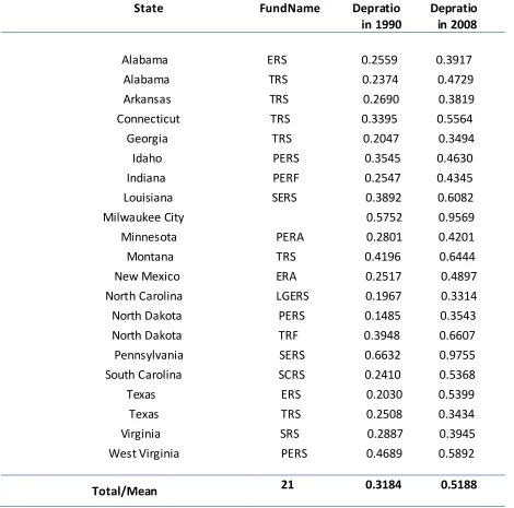
State FundName Depratio Depratio in 1990 in 2008
Alabama ERS 0.2559 0.3917 Alabama TRS 0.2374 0.4729 Arkansas TRS 0.2690 0.3819 Connecticut TRS 0.3395 0.5564 Georgia TRS 0.2047 0.3494 Idaho PERS 0.3545 0.4630 Indiana PERF 0.2547 0.4345 Louisiana SERS 0.3892 0.6082 Milwaukee City 0.5752 0.9569 Minnesota PERA 0.2801 0.4201 Montana TRS 0.4196 0.6444 New Mexico ERA 0.2517 0.4897 North Carolina LGERS 0.1967 0.3314 North Dakota PERS 0.1485 0.3543 North Dakota TRF 0.3948 0.6607 Pennsylvania SERS 0.6632 0.9755 South Carolina SCRS 0.2410 0.5368 Texas ERS 0.2030 0.5399 Texas TRS 0.2508 0.3434 Virginia SRS 0.2887 0.3945 West Virginia PERS 0.4689 0.5892
Table 7: Mean values of the number of beneficiaries and workers for all of the pension
plans and those have larger dependency ratio in 2008 than in 1990
1 All pension plans
Year
Beneficiaries
Workers
Dependency Ratio
1990
2,973,311
8,929,950
0.333
2008
6,002,982
12,029,028
0.499
2 Pension plans those have larger dependency ratio in 2008 than in 1990
Year
Beneficiaries
Workers
Dependency Ratio
1990
27,456
96,214
0.285
Figures
Generated from the sample
Figure 2: The Development of the Variables from 1990 to 2008 0
0.2 0.4 0.6 0.8 1 1.2 1.4
1990 1992 1994 1996 2000 2002 2004 2006 2008
Funding Ratio
Dependency Ratio
Formula Multiplier
REFERENCES
Brainard, Keith. 2007. Public Fund Survey Summary of Findings for FY 2006. NASRA, October.
http://www.publicfundsurvey.org/publicfundsurvey/pdfs/Summary%20of%20Finding
s%20FY06.pdf
Clark, Robert and Lee A. Craig and John Sabelhaus. forthcoming. State and Local
Retirement Plans in the United States, London: Edward Elgar.
Myers, Randy. 1998. ―Stock Market Faces an Uncertain 1998,‖ Nation’s Business. 21 February
National Bureau of Economic Research, Business Cycle Dating Committee. 2011. ―US Business Cycle Expansions and Contractions‖. Cambridge, MA: National Bureau of Economic Research
National Conference of State Legislatures. 2009. State Budget Update: November, 2009. NCSL Report.
Rauh, Joshau and Robert Novy-Marx. 2011. ―Policy Options for State Pension Systems and Their Impact on Plan Liabilities,‖ National Bureau of Economic Research Working Paper No. 16453, Cambridge, MA: NBER.
Schieber, Sylvester J. and John B. Shoven. 1999. The Real Deal: The History and Future of
Social Security. New Haven: Yale University Press.
Schmidt, Daniel. 2009. ―2008 Comparative Study of Major Public Employee Retirement Systems.‖ Wisconsin Legislative Council Report. Madison, WI: Wisconsin
Legislative Council.
Wisconsin Legislative Council. Various years. Comparative Study of Major Public Employee