MAINTENANCE OF GENETIC VARIABILITY UNDER THE JOINT EFFECT OF MUTATION, SELECTION AND RANDOM DRIFT

(1)

EFFECT O F MUTATION, SELECTION AND RANDOM DRIFT*

WEN-HSIUNG L I

Center for Demographic and Population Genetics, University of Texas Health Science Center at Houston,

Houston, Texas 77025

Manuscript received August 1, 1977 Revised copy received March 31, 1978

ABSTRACT

Formulae are developed f o r the distribution of allele frequencies (the frequency spectrum), the mean number of alleles in a sample, and the mean and variance of heterozygosity under mutation pressure and under either genic or recessive selection. Numerical computations are carried out by using these formulae and WATTERSON’S (1977) formula f o r the distribution of allele frequencies under overdominant selection. The following properties are observed: (1) The effect of selection on the distribution of allele frequencies is slight when 4Ns 2 4, but becomes strong when 4Ns becomes larger than IO, where N denotes the effective size and s the selective difference between alleles. Genic selection and recessive selection tend to force the distribution to be U-shaped, whereas overdominant selection has the opposite tendency. (2) The mean total number of alleles in a sample is much more strongly affected by selection than the mean number of rare alleles in a sample. (3) Even slight heterozygote advantage, as small as 10-5, increases considerably the mean heterozygosity of a population, as compared to the case of neutral mutations. On the other hand, even slight genic or recessive selection causes a great reduction in heterozygosity when population size is large. (4) As a test statistic, the variance of heterozygosity can be used to detect the presence of selection, though it is not efficient when the selection intensity is very weak, say when 4Ns is around 4 o r less. A model, which is somewhat similar to OHTA’S (1976) model of slightly deleterious mutations, has been proposed to explain the following general patterns of genic variation: (i) There seems t o be an upper limit for the observed average heterozygosities. (ii) The distribution of allele frequencies is U-shaped for every species surveyed. (iii) Most of the species surveyed tend to have an excess of rare alleles as compared with that expected under the neutral mutation hypothesis.

selectionist us. neutralist contmversy over the maintenance od genic

ation ion

in natural populations has now continued unabated for ten years (see LEWONTIN 1974; NEI 1975 for reviews). What is needed to resolve this controversy is a theory by which the statistical properties of a population under the joint effect of mutation, selection and random drift can be examined thor- oughly. Only by so doing can one evaluate the relative importance of these three

(2)

factors i n the maintenance of genetic variation or construct suitable statistics f o r

testing hypotheses. Actually such a theory can be developed by using

WRIGHT’S

(1949a) formula for the joint distribution of multiple alleles, but only very recently have workers begun to do so. Using this formula,

WATTERSON

(1977) has developed a statistical theory for the case of symmetrical overdominance among multiple alleles, and

I

(LI 1977) have developed a similar theory for the cases of genic selection and recessive selection;

WATTERSON

(1978) has later studied more general cases. In LI (1977), however,

I

have presented only a short summary of some of my findings. Here

I

present a detailed account. In Section I, I derive formulae for the distribution of the mean number of alleles at different frequencies or the frequency spectrum, and formulae for the mean number of alleles in a sample. Numerical computations are carried out by using these formulae and that of WATTERSON (1977) to see how selection changes the shape of the distribution of the mean number of alleles at different frequencies. Numeri- cal computations are also carried out for the expected number of alleles whose sample frequency is equal to or less than q, 0 5 q I 1. I n Section 11, I develop formulae for the mean and variance of heterozygosity. These results, together with that of WATTERSON (1977), are applied to study how the average heterozygosity of a population changes with population size. The present result is also used to examine the effect of selection on the variance of heterozygosity. In

Section 111, I discuss the implications of the present findings for the maintenance of protein polymorphism.

DISTRIBUTION O F ALLELE FREQUENCIES

One of the most useful methods of describing a population is the distribution of allele frequencies or the frequency spectrum, which is conventionally denoted

by

@(x).

Actually, @(z) is not a distribution in the probabilistic sense, but has the meaning that @ (z) dx represents the expected number of alleles whose frequency is between

x

-

dx/2 and x f dx/2. Although a more precise term for

@(z) is the distribution of the mean number of alleles at different frequencies,

I

follow the convention of calling

@(x)

the distribution of allele frequencies. The distribution @(z) for the case of neutral mutations has been studied by WRIGHT

(1949b)

,

KIMURA and CROW (1964)

,

KARLIN and MCGREGOR (1967), and NEI and LI (1976), while that for the case of overdominant selection by WATTERSON

(1977). Here, I study the cases of genic and recessive selection. Before this, I

review WRIGHT’S (1949a) formula for the joint distribution of multiple alleles, which is essential to this study.

Consider a random-mating population of effective size N . Let the number of possible allelic states at a locus be K , and let Ai denote the ith allele and xi its frequency. Let the selective value of genotype A,Aj be w,j, which is assumed to

be constant over time, and let m(z,,

.

. .

,xK) be the mean fitness of the population. Assume that in each generation A , mutates to Ai with probability uf,,

j #

i.

I n practice, it is likely that u j , is a function of both Ai and A,, but no solu-

(3)

35 1

special case where uji = ui for all

j

#

i,

WRIGHT

(1949a) has obtained, using some heuristic arguments, the following formula folr the equilibrium joint probability density for the first L = K - 1 gene frequencies:

where ai = 4Nui and xK = 1

-

x1

-

.

. .

-

xL.

A formal mathematical proof of

this folmula has later been provided by KIMURA (1956),

WATTERSON

(1977) and LI (1977), independently. Note that the mutation rate per gene per generation from

A i

to all other alleles is ul

+

. .

.

+

vi+l

f

. . .

+

V K or U

-

vi,

where U = U ,

+

.

+

ui

+

.

. .

+

U,. If ui is the same for all

i,

then U

-

vi = U

and ui = u / L for all

i.

This symmetrical case has h e n known as the K-allele model (WRIGHT 194913; KARLIN and MCGREGOR 1967; KIMURA 1968). The normalizing factor C in formula (1) is determined by the relation

J

.

.I,

+(xl,

. . .

,xL)dxl

.

. .

d.xL = I,

(2)

where the integration is over the region defined by

R:

O I ~ i 5 1 , X I +

...+

~ L 5 1 .

This multiple integral may be evaluated by following WATTERSON’S (1977) method, if the wij’s are given explicitly.

The form of formula (1) is amazingly simple. Thus, to determine the joint probability density, we need only know the mean fitness of the population and the mutation rate (vi) to Ai. This makes formula (1) also applicable to the case where Ai denotes a class of equally fit alleles instead of a single allele. To see how this works, we consider the following simple example. Suppose that the last

( K

-

j ) allelic states are equally fit and let us regard them as a single class Bj+l. Let Bi = Ai,

i

= 1,

. . . ,

j . Let yi be the frequency of B, and U + be the mutation

rate to B,,

i

= 1 , .

. .

,

i

-I- 1. This implies y , = x i and U * =vi,

i =

1,

. . .

,

i ;

~ j =xj+l+ + ~

.

+

x K and u , + ~ u , + ~

+

.

+

uK. Obviously

W ( X ~ ,

. .

.

,

x K )

can be written as m(yl,.

. .

,

y3+1). Then, formula (1) says that the joint distribution of yl,

.

. . ,

yj is given by

i + l .IIVU*-l + ( Y l , .

.

. ,

y j ) = C’W2’v 2=1 ,II y i

.

This can be verified by following the simple proof procedure of formula (1) given by LI (1977) (see also

KIMURA

1956; WATTERSON 1977). In particular, it is easy to see that when j = 1, this formula becomes identical with that for the diallelic case where the mutation rate from B , to B, is u1 and that from B , to B, is uZ (WRIGHT 1949a).

Genic Selection

We begin with the general case. We assume that the mutation rate, U = U - ui,

(4)

W e use the notations: 0 = 4Nv = La: and 6’ = 4Nu = 6

+

a:. Let the selection coefficient for the

ith

allele be ai so that the relative fitness of genotype AiAi is given by w L j = 1

+

a,

+

aj. Then

f =

1

+

2alzl

+

.

. .

+

2aKzK and

K a-1

+(Zl,.

.

,XL) =CW2N II xi

,

(3)

where (?”) is the binomial coefficient and the summation

z

is over all vectors ( n ) =

(G,

.

. .

,

n K ) of non-negative integers such that n,

+

. . .

+

nK = n. Using the Dirichlet integral formula (JOHNSON and KOTZ 1972) and the relation given by (2), we find that

( n )

2N n1

C-l=

z

(2N)n!2n

z

II [ai r ( n i +a)/~i!]/r(rt+6’).

n=o 7 1 ( n ) 1

To derive

@(x),

we focus our attention on a particular allele, say Ai, and compute the probability,

+,

(xj) dxj, that the frequency of A , in the population is in

(xi

-

dzj/2, zj

+

dzj/2). Note that +j (zj) is the marginal probability density

for x j , and therefore

+j(zj) =

I..

.J

+(xl,..

.

,xL)dxl..

.

dxj-ldxj+l..

.

dxL, ₍₄₎

where the integration is over the region

R’:

0 5 xi 5 1 - xj, 5 1

-

xi,

i

#

j .

Use of the transformation

z i = z ; / ( l -xi),

iZj,

enables us to apply the Dirichlet integral formula to evaluate the multiple integral of (4) and we obtain

Since there are K allelic states,

The subscript of 5 is now dropped because we are concerend with the mean number of alleles at a given gene frequency class, n o t any particular allele or alleles. Note that without losing generality, we can assume aK = 0, and formula

( 5 ) is simplified to some extent.

Formula (5) is general but it is useful only when K or the magnitude of the

(5)

I n order to make detailed computations feasible, we consider the following models.

Suppose that there are three classes of alleles, within each of which there are a number of equally fit alleles. Let the number of allelic states for the first, second, and third classes be I , M , and Q = K - I - M , and let the selection coefficient be s1 for the first-class alleles, sz for the second-class alleles, and 0 for the third-class alleles; s1 and s2 can be positive o r negative. %(z) can be obtained by putting these conditions into formula ( 5 ) , but this creates the same compu- tational difficulty as that of formula

( 5 ) .

The following approach overcomes this difficulty. Let

y l = 5 1

+

.

+

XI,

y z = x 1 + 1 + . . . + x 1 + a f , uz = M v / L ,

e2

= 4NUz = M , ~ ,

U1 = I v /L,

e,

= 4NUl= iff,

y3 = 1 - yl - y2, ~3 == Qu/L7

e3

= 4 N ~ 3 Qa,

where y. is the sum of the frequencies of the ith class alleles and ui is the sum of

mutation rates to the ith class alleles. Note that formula

(5)

now becomes = I+i

(x)

+

M+r+i (2)

+

Q + K ( ~ ) . (6)

Note also that we may alternatively let the selection coefficients for the first-, second-, and third-class alleles be 0 , t2, and tR, or r1, 0, and r3 so that

FV

can be expressed i n terms of the yi's in three different ways:

(7a) (7b) (7c) where t 2 = (sz-sl)/(l +2sl), t 3 = - S 1 / ( 1 +2s1), r l = (sl-sz)/(l +2sz), and

7-3 = - s 2 / ( 1

+

2s2). To evaluate +1

(xl)

,

we consider the joint distribution of

xl,

. .

.

,x1-1,yZ,y3, and write as (7b). As mentioned in the remark on formula

( 1 )

,

this distribution can be written as

w

= 1

+

2s,y,+ 2s2yz

= (1

+

2S1) ( 1

f

2tzyz

+

2t3y3)

= (1

+

2Sz) ( 1

+

2riyl

+

2T-3y3)

+

(XI7 * * * ,xI--lrYZ?y3) = Clr (a)"(

+

2t2y%

+

2t3y3) I

x

yze2-ly3&-l

n:

1

x p ,

( 8 )

multinomial expansion and the

r(nl

+

ez)r(n2

+

e,).

where C , is the nolrmalizing constant. Using Dirichlet integral formula, we find that

2 N n!2" t 2 n d 3 n ~

cl-l

=

x

);( E-

r ( n

+

e')

( n ) nl!n2! n=O

From formula ( 8 ) , we obtain

Zh

+ 1 ( ~ ) = Clr(lff)-lxwl(l

-

n!2"

z)B-l

z

(") ( 1 -x)"

(6)

(To keep the notation simple, we have written here and shall write +i(xi) as +i(z) when it creates no ambiguity.) On the osther hand, to evaluate

+l+l(xI+l),

we consider the joint distribution of yl,xl+l,

.

, ~ ~ + ~ - , , y ~ , and write

@

as (7c).

In the same manner, we obtain

2N n!2"

+ K ( ~ ) =

C3r(a)-1~~i(1

-

z)o-l

z

(") (1

-x)"

n=o n

r ( n + e >

Putting together (6), (9), (1 1 )

,

and ( 13), we have

x [e1Clt2nlt3nZr(n,

+

e 2 ) r ( n 2

+

e,)

+

02C2rln~r3"~r(nl

+

e,>r(n,

+

e,)

+

e3c3Sln1S2nzr (n,

+

e,)

r

(n2

+

e,)

I.

(14)

If )4NsiI

<<

N,

i

= 1,2, formula (14) may be approximated by .p-1(1

-

s) 8-1 2~ (1

-

z)" 1

a(x)

=

z

z-

r ( 1 + a ) n=o r ( n + O ) ("1 nl!n2!

x [elc1T2n1T3n2r(n,

+

e 2 > r ( n 2

+

e,)

+

e,C,Rln~R,nZr(nl

+

e l ) r ( n 2

+

6,)

+

e , ~ , ~ , n ~ ~ , ~ ~ r ( n ,

+

e,)r(n,

+

e,)],

(14')

where Si = 4Nsi, Ti = 4Nt6, Ri = 4Nr4, and 2 N

c-1

= I; r ( n

+

e y

z

T2n1T3nzr(n,

+

e,)r(n,

+

e3>/(nl!nz!),

(7)

355

2N

C-l=

x

r ( n

+

e y

z

SlnlSZnZr(nl

+

& ) r ( n ,

+

6,)/(nl!n,!).

3 ll.=o ( n )

The same approximation applies to all of the following formulae, but will not be repeated (see LI 1977). However, all numerical computations of this study are carried out under this approximation.

The key difference between formulae

(5)

and (14) is that in the latter for

every n only the possible alternatives of nl and n, are to be considered, i.e., the summations

z

are now univariate summations over nl = 0, 1, 2,

. .

.

,

n, with n, E n

-

n,. Since this is true for any

K,

the limiting case of infinitely many

alleles is just a special case. Indeed, to apply formula (14) to the model of infinite alleles (WRIGHT 194913; KIMURA and CROW 1964), we simply put a = O and 0' = 8. This remark applied to all the following results.

(n)

The mean number of alleles in a population is given by

assuming that the effective populatioln size,

N ,

is equal to the actual size. (We use 1/4N instead of the conventional value 1/2N as the lo'wer limit of integration because it allows a continuity correction.) When

K

is finite,

r 1 / 4 ~

= K -

+((X>dx,

in which the last integral represents the mean number of alleles that are not present in the population.

We now study the mean number of alleles in a sample. We consider only the case of infinitely many alleles, since the result for this case is somewhat simpler in form and numerical computations are usually carried out under this condition. OHTA (1976) shows that the mean number of alleles whose sample frequency is less than or equal to q is given by

x)

(x)

dx,

where 2n is the number of genes sampled,

is

= 2mq, and

[is]

denotes the integral part of

i8.

(If we define n4 as the mean number of alleles whose sample frequency is less than q, then

[is]

= 2mq

-

1 if 2mq is an integer, and

[is]

= the integral part of 2mq if otherwise.) We assume that N

>>

m so that the lower limit of integration can be replaced by 0 with a good approximation. Using the relation

( 2 m - i + l ) i i ( 2 m

+

n

+

e

- i)

(8)

where (a)i = a ( a

+

1)

.

. .

( a

+

i

- I ) , we find that ZN n!2" ( 2 m - i i l ) i 1

n=o r ( n +

e )

i=i i ( 2 ~ ~ + n + e - i ) ~ (n) nl!nz!

n4 = 2 :) (.

z

z-

x

[e1Clt2nlt3nzr (n,

+

e,)

r

( n ,

+

e,)

+

ezCz~lnl+3n2r ( n ,

+

e,)

r

( 12,

+

e,)

+

e 3 c 3 ~ l ~ l s z n 2 r ( n l

+

e,)r(n,

+

e , ) ] .

(15)

If q = 1, the above formula can be simplified by noting that[i,] = 2m and

The same substitution applies to the case of recessive selection below (formula (24) ) .When q = 1, formula (15) represents the expected total number of alleles

in a sample of 2m genes, and it reduces to formula ( 11) of EWENS (1972) if all mutations are neutral.

The formulae for the case of k ( k

>

3) classes of alleles can be written down immediately by analogy, but computer computation soon becomes impracticable as the number of classes increases. On the other hand, the case of two classes of alleles is just a special case of three classes of alleles, Since this case is of particular interest, because of its simplicity, we consider it in some detail. Let the selection coefficient be s for the first-class alleles and 0 for the second-class alleles. This is equivalent to assuming that s1 = s and sz = 0. Since there are no third- class alleles, 8, = 0. Putting these conditions into formulae (14) and (15), we obtain

p - 1 ( 1 - 2) B-1 2 N 2"(1 -z)n r ( l + a ) n=o

r ( n

+

0 )

@(z) =- 2: (2")

where t = - s / ( 1

+

2s). Recently, WATTERSON (1978) has also studied the case of two classes of alleles under genic selection and has obtained a n approximate formula for @(z), assuming that S = 4Ns is very small. Incidentally, formula

(9)

first allele the type allele and gave a n estimate for the mean number of deleterious alleles present in the population. He assumed that each gene mutates at the rate of U per generation and that the rate of backward mutation from all other alleles

to any allele is ul. This is equivalent to the assumption that the number of allelic states is K = u/ul

+

1. H e obtained the following approximate formula f o r the mean number of deleterious alleles in the population, assuming S large.

The general formula for nd is obtained by integrating the second term of (17) from 1/4N to 1 and by noting that

el

= a and 8, = 8.

2 N r ( n + a )

r ( l + a ) "=O r ( n +

e )

c,

z

(") (2s)"

e

na= KB- 1 -

Formula (20) applies to any values of

N

and s, but it is more complicated than

WRIGHT'S

(1966) formula.

It

is therefore interesting to find the condition under which

WRIGHT'S

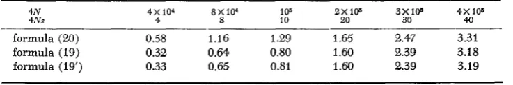
formula holds approximately. WRIGHT considered u1 = 0.25 x and 0.25 x 10-lo, and found that nd is almost the same for both values of u1 if U = 1k6, s 2 and N 2 IO5. Since the approximation is more accurate when u1 is larger, I have used the smaller value u1 = 0.25 x 10-lo i n computing Table 1. I t is seen from this table that WRIGHT'S formula holds approximately when S is larger than 10 and that formula (19#) gives a close approximation to formula (19).

Recessiue Selection

W e consider two classes of alleles and assume that the number of allelic states is I for the first class and M = K - I for the second class. Let the relative fitness of genotype AiAj be 1 - 2s if

i,j

>

I , and be 1 otherwise. This means that the second-class alleles are completely recessive. The joint distribution of xl,

.

. .

,xI-l

and y z is

TABLE 1

Mean number of akleferious alleles in a population of size N

4N 4 x 104 8 X l P 105 2 X I W 3X108 4X 105

4Ns 4 8 10 20 30 40

2.47 3.31

3.18 3.19

1.29 1.65

0.64 0.80 1.60 2.39

1.60 2.39 0.58 1.16

0.32

formula (20) formula (19)

formula (19') 0.33 0.65 0.81

(10)

2 a,

_r

_(2n

+

e,)

c-1

=

z

(") (-2s)"

1 n=o n

r

(2n

+

e#)

'

from which we obtain

Similarly we obtain

K

4

( Y ~ , Z ~ + ~ ,

. . .

,xK)

= C,r (a)-"( 1

+

2s,yl

+

2 q ) 2Ny:-1

,

(22)

where s1 = 2s/ (1 - 2s)

,

sz = -s/ (1 - 2s). Thus,

a(5)

=

Z@,(x)

+

M @ K ( Z )

The formula corresponding to formula (15) is

(11)

Numerical Examples

(A)

Distribution of allele frequencies: Before considering numerical results, let us examine analytically the folrm of the distribution of allele frequencies under various types of selection. The distributions of allele frequencies for the cases of genic and recessive selection are given above, while that for the case of symmetrical overdominance is given by

@(x)

= est-l(i - x)ble-~zzW(,(l

-

x ) z , 8 ) / W ( ~ , 8 ) , (25

1

where U = 2Ns ( WATTERSON 1977). This formula is derived under the assump-

tions that the relative fitness is 1 for all heterozygotes and 1

-

s for all homcny- gotes, that the number of allelic states is infinite, and that 12Nsl

<<

N . The C i , n constants can be computed by use of the following recursive formula:

starting with Cl,n = ( 2 n

-

l)!/n! (STEWART 1976; WATTERSON 1977). We note from formulae ( 5 ) , (14), ( 2 3 ) , and ( 2 5 ) that regardless of the type of selection all the distributions under the model of infinite alleles have the common factor

st-, ( 1 - s) B-I, as does the distribution for the case of neutral mutations:

~ ( z ) =

exqi

-

Z ) B - ~

.

_{( 2 6 )}

Thus, in all cases the value of @(x) at s = 1 is infinite if 8

<

1 , finite if 8 1, and 0 if 8

>

1, while that at s = 0 is always infinite. It is also easy to see that

@(s) given by ( 2 6 ) is U-shaped if 8

<

1 and L-shaped if 8 2 1. By continuity, the distribution under very weak selection pressure should be of the same shape as that for the case of neutral mutations; numerical results indicate that the shape of @(s) is not much affected i f s 5 1/N. These few properties are all that can be inferred analytically. To have a deeper understanding, numerical computations are necessary. A particular effort to be made is to see under what situation a U-shaped distribution can be obtained, because this shape of distribution is universally observed in nature for protein loci (unpublished studies of CHAKRA- BORTY,

FUERST

and NEI)

.

In all examples in this section, the model of infinite alleles is used. The examples given in Figures l a and I b are intended to show the effect of selection on the shape of the distribution of allele frequencies. The selection intensity is

4Ns1 20 and 4Nsz = 10 for the case of three classes of alleles under genic selection, 4Ns = 20 for the case of two classes of alleles under recessive selection and 2Ns = 10 for the case of overdominant selection. In the case of genic selection, 8 is divided into 8, = 0.018, O2 = 0.098, and 8, = 0.908; 8 / 2 = 2Nv represents the number of new alleles appearing in each generation, of which 8,/2

(12)

360

O 2 = 0.990. I n Figure la, 6' = 0.1 for all cases. The curve for neutral mutations is U-shaped, as expected. The curve for genic selection is also U-shaped but there are fewer intermediate- and low-frequency alleles and more high-frequency alleles as compared to the case of neutral mutations. To avoid crowding, the curve for recessive selection is not shown in Figure la, but it is U-shaped. The curve for overdominant selection has a peak at x = 0.41 and is far from being U-shaped-there are more intermediate- and low-frequency alleles and fewer high-frequency alleles as compared to the case of neutral mutations. Thus overdominant selection and genic selection have opposite effects on the shape of the distribution of allele frequencies. The mean heterozygosities for the cases of overdominant selection, neutral mutations, and genic selection are 0.485, 0.091, and 0.012, respectively. In Figure lb, 6' = 1. Now only the curve for genic selection is U-shaped. However, the curve f o r recessive selection is nearly U-shaped and shows a similar tendency as that for genic selection. The curve for overdominant selection is again far from being U-shaped. As expected, the curve for neutral mutations is L-shaped. The mean heterozygosities for the cases of over-

5

4

3

2

1

0

0 .5 1

G E N E F R E Q U E N C Y

FIGURES l a and 1b.-Distribution of allele frequencies under various types of selection. The ordirlate denotes @(z), which has the meaning that + ( z ) d z represents the expected number of

(13)

dominant selection, neutral mutations, recessive selection, and genic selection are 0.697,0.500,0.238, and 0.1 14, respectively. The bearing of the above findings on protein polymorphism will be discussed later.

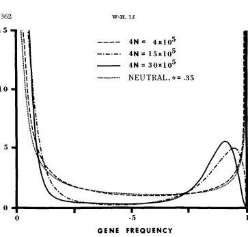
Figure 2 shows the effect of population size on the distribution of allele frequencies for the case of three classes of alleles under genic selection. The parameters used are s1 = s2 = 4 2 , U 1.12

x

u1 = 0.02 X us = 0.1 X

and u3 = When 4N = 4

x

lo5, the curve is U-shaped. This is expected because B = 0.448 is smaller than one. The curve for 4N = 15 X lo5 has a peak at z = 0.95, but there are now fewer intermediate-frequency alleles and more low-frequency alleles than those for the previous case. As expected, $(z)

becomes 0 at z = 1 since 0 is now 1.68. When 4N increases to 30 X lo5, the peak becomes higher and moves to the left. This tendency will continue as population size increases-when N becomes infinite, all alleles will be concentrated near

x

= 0. Although the three curves f o r 4N = 4 X IO5, 15 X IO5, and 30 X IO5 look different, they yield very similar mean heterozygosities: 0.268,0.250, and 0.269.

1 5

10

5

0

P N v = 1

OVERDOMINANT

I

...

NEUTRAL

----

R E C E S S I

V E

I

G E N I C , 3 C L A S S E S

!

I

I I

I I I

0 .5 1

GENE FREQUENCY

Figure Ib, 6 = 1. Overdominant selection: U = 2 N s = _{10. Recessive selection:}4Ns = _20,6, =

(14)

W-H.

1 5

1 0

5

0

-

4 N = 3 0 x 1 0 5

...

N E U T R A L ,

e = .35

0 . 5 1

GENE FREQUENCY

FIGURE 2.-The effect of population size on the distribution of allele frequencies under genic selection. The ordinate denotes @(z), which has the meaning that +(x)dx represents the expected number of alleles whose frequency is between z - dx/2 and z -I- &/2. Mutations are divided into three classes with u1 = 0.02 x 10-6, u2 = 0.1

x

1 6 6 , and u s = 10-6, s1 = 10-5, and

sp = sl/2. The neutral case is for comparison. For details, see text.

Let us now consider a hypothetical population in which mutations are strictly neutral, but the mean heterozygosity

&

at equilibrium is about the same as those of the above three populations, say

9

= 0.26. From this

a,

we obtain 0 = 0.35 by

using the relation

H =

e / ( l

i-

e )

(KIMURA

and CROW 1964). Using this 0 value and formula (26), we obtain the curve for the case of neutral mutations (Figure 2 ) . This cunie is very similar to the first curve, but different from the other two curves. Thus, the distribution of allele frequencies may be used to detect weak selection in large populations where the effect of random drift is relatively weak. One general property is that for a given level of mean heterozygosity there is an excess of rare alleles in the case of genic selection compared with the case of neutral mutations. On the other hand, in the case of overdominant selection the number of rare alleles tends to be small, while the number of intermediate- frequency alleles tends to be large compared with the case of neutral mutations.

(15)

given in Figure l a is 0.485, which is close to the value of 0.500 for the case of neutral mutations given in Figure lb, but there are fewer rare alleles and more intermediate-frequency alleles in the former case than in the latter (note the difference in scale for the ordinates). It should be noted that in this method of comparison the distribution for the model of neutral mutations is computed by using 0 =

p/(

1

-

g ) .

Here,

I

?

is the expected heterozygolsity for the population under study, while in practice it refers to the observed average heterozygosity.

If

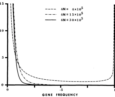
the number of rare alleles for the population under study is larger (smaller) than that for the model of neutral mutations, then we say there is “an excess (deficiency) of rare alleles.” This terminology is used in this sense throughout the present paper.

In Figure 3 we plot the distribution of the mean number of the third-class (most disadvantageous) alleles at different frequencies for the three cases of genic selection shown in Figure 2. It is seen that when 4N =

4 x lo5

and

4Ns, =

4,

the third-class alleles are spread over the whole range of gene fre-

1 5

1 0

5

0 I I I I I I

I

I I

I

----

4 N = 4 x 1 0 5

-.-.-.

4 N = 1 5 x 1 0 5 4N

=

3 0 x 1 0 5

0 .5 1

GENE FREQUENCY

FIGURE 3.-Distributions of the number of the third-class (most disadvantageous) alleles under genic selection. The ordinate denotes (P3(x), which has the meaning that @.,(z)dx represents the expected number of the third-class alleles whose frequency is between x - dx/2 and

(16)

364

quency, including the fixation class. But when 4 N increases to 15 X lo5 so that 4 N s , = 15, virtually none of the third-class alleles have a frequency higher than 0.3. As the population size increases more, the third-class alleles are pushed further down to lower frequencies. Thus, slightly deleterious mutations are able to spread over the whole population when N is of the order of l/s o r smaller, but are kept in low frequency when N is one order larger than l/s, where s is the selection coefficient against these mutations.

A property of prime importance emerges from the above results: the higher the potential for mutations to persist in the population, the lower the probability for @(z) to be U-shaped. (The potential is determined by N and the selective values of the mutations.) This is because the sum of allele frequencies must be one, and therefore the probability f o r any of the allele frequencies to be close to one becomes small when the number od alleles becomes large (cf., Fig. l b ) . Obviously the distribution @(z) cannot be U-shaped if there is no allele with frequency close to one. The distribution also cannot be U-shaped if there exists a peak at an intermediate frequency. Such a peak can arise if there is a force to keep some alleles at intermediate frequencies (cf., Fig. l a ) . I t can also arise because of the accumulation of a large number of low frequency alleles (cf.,

Fig. 2).

I n the light of the above findings, the property of the distribution of allele frequencies under various situations can be recapitulated as follows: (1) For neutral mutations, there is no selective force to retain alleles in the population, but there is also no selective force to eliminate them so that alleles can become extinct only through random drift or mutation. Thus, the distribution is U-shaped

if new alleles arise at a rate lower than one in every two generations, i.e.,

0 = 4 N v

<

1, but it becomes L-shaped if new alleles arise at a higher rate,

(17)

increases. ( 3 ) “Purifying” (or “negative”) selection, which includes genic selection, recessive selection, etc., tends to force the distribution to be U-shaped, for it is rather effective in eliminating disadvantageous mutations or in keepng them in low frequencies. Under this type of selection, the distribution is U-shaped if 6‘ 5 1. When 6’ becomes larger than one, ~ ( z ) becomes 0 at z = 1, but has a peak at a high gene frequency (see Figure 2). The location of this peak depends on the intensity olf selection as well as the magnitude of 6’. If it is clolse to z = 1, the distribution, when plotted as a histogram, may become U-shaped. For example, the histogram for the curve with 6’ = 1.68 in Figure 2 is U-shaped if the range of gene frequency is divided into ten equal intervals. This example shows that by incorporating even tiny selective differences such as s1 = and s2 = l O ~ ~ / 2 into the model of selective neutrality, a U-shaped histogram can be obtained even

if 6‘ is substantially larger than 1. I n natural populations a U-shaped histogram may be obtained for an even larger 6’ value, because the majority of mutations are perhaps more deleterious than s = Note also that in practice only a finite number of genes are sampled from the population, so that low-frequency alleles are less likely to be observed than high-frequency ones. This sampling effect tends to move the aforementioned peak closer to z = 1. Numerical computations show that this effect increases the chance of observing a U-shaped histogram, though only to a small extent. Thus, under purifying selection the observed distribution, which is generally plotted as a histogram, can be U-shaped even if 6’ is considerably larger than one, say of the order of 10. However, i t is unlikely that a U-shaped distribution can be observed if 6‘ is much larger than one, say of the order of 100 or larger, unless a n overwhelming majority of mutations are very deleterious so that they are quickly eliminated from the population or kept in exceedingly low frequencies.

(18)

366

- U )

3 ;

&

"

a

G

CA v 2 % .E E 2 W E % a ; : U

8 .s

*

'2

-

.v U I: 1-

g

.h ~m

2 "

B

5

E:

W-H. LI

3-g d

;I

3.g

0 c D 3 * w m m m m l n m v m 9 z o

$ 2

0 0 o i 0 * a 0 w a 0 3 l n 3 w K ) 9 $ " - ! " " 9 9 5 ? 9 9 9 " O 2 $

=

z a "I :.a

*

! 2

1 @

D

M

~ F & 3 i q ~ ~ ~ g & @ s 2 ~ + g

Z O Q

I I a a K ) + - I - M w ~ w w w w O O t $ 5

- w c 3 ~ & s & ~ & & 6 s & G - ~ - - *

+.' 0

Jp:

H?-E

y~~z~?~~~~~~~

0,

q

0,:s 8

E:f

**d * " m d d m d + d w m c d**

g

k 2 '1 q 0 'IF 0 q ". 3 q ". .? ".

g

F g 4

z z c z ~ z ~ z ~ ~ c c z c

&

E

0 q h q

T

a, '1 ". w 0 q 0 q

8

2

o* oK)*K)mw*hwa$3maK)

a B

al

3 al 6 - 7

n--nn---nnn--- 3%'

M g ? q * y t . ' 1 ' 1 0 q q q q w o g f i

bl

:

so

I1 a a K ) * * K ) ~ a w w w h $ ~

& u s

0 m 1 1 h c o v ) o a m m e w q g q q T

$ $

f

E

;i"

v v v v v v v v v v v v v v c . 2 3

0 r?rS?t.4"c?tO""cn0"~ " 2 U)-

oK)*K)mb*cmwc33mfx~

5 2

2

2 . g h m m m m w a 0 m " v ) ~ a h E

8 2

g s

**owmm~~zhz-+mco~**

-2s

E Ggd E "

F?: E

?j S I 2

w " T ? + ? a W ? h h ? 9 8

p z

$7-

nqg

&;da-$-ddc&&G&;b F:

?a

q a o ?

03%0.?"-!c?" % b $ %

4

"I?

2 a $

i!z+:

A d o 0 0 0 0 0 0 0 0 0 0 0 0 0 0

3 %

c.l ILI! v v v v v v v v v v v v v v fi

-

+

-q " -q -q c n w u ? -q 0 -q w " . r ? -q & J O E 2 V I 2

?$U)

2

a w w m - m m m o a m w m a E G O

h K ) v ) O h " M m m h K ) * m c c , $ t i

b o ' 1 q 0 ' 1 0 q . ? 0 1 . ? - !

_c

_~

_z

.-!

_~

z

_{' 3 6}

_~

q

_~

_g

_c

_~

_z

h * Q * * W * m - * " o v ) Q E

c ? r ? ~ q " q q o 0 q * " . q " a g g

O" o o c 4 0 - a o w K ) ~ 3 M " a M 3 v1 g

.2

9

fi

b.3 a w h * h h & w M b m 3 * 0 a g . -

a z :

$ 7 4 =:

+ o o ~ o o ~ o o . + o o - o $ h a l o

s?$s?gF?$s?F?I:-I:oz?s?s?F?s- II

p

0 3 2 "

0 0

i ? ; 2

g

;E

!

B E

!

E

n--nnnnn--nnnn a~ 8 3

a

" h - a h h w w 0 0 - a

II

3

-- h w K ) m h * m m K ) w * E 5

_mGM w & m w w - " a ~ a m

a m w

0 c j 0 s c j 0 3 a 0 3 a

-

3 ro

O a h ~ a O v ) w m O a * K ) h

U) "E;

e 5 0 %

5 % q 0 w 0 0 q m m T r ? " . " w q

el a %

a 0

nn-nnnnnnn-nnh

O w m * l n O 3 3 - h h h * 3

"

2

0

-

0 3 a 0 3 m o 3 a

-

a CO

0 0 0 0 0 0 0 0 0 0 0 0 0 0

mm ** i^ K)" a- g

*"

K)* a" +- mm a*

*-

*"

0 M 0 0 ln 0 0 ln0 0 Po 0 0 K)

o o ~ ~ t . m o h m - a m a + o ~ )

0 0 a 0

-

a 0 3 K) * 3 K) 3 a Po

me m

+z '0 3

0 3 . 0 < < 0 A A 0 . A & s A d

*

e 5

-n,-,--n-n-nnn-n

2

$ 1 1

k

w

$gtn.+

3"wLv)K)hw-w*3go-+g* .s al U)

E $

z g 2.5 o o a 0 - l n o G M - ~ M - c 4 * qicqqqmqq m 0 0 \ n l r ? . ?

$

$ 2

0 m II

z 2

5 - .*,

0 %

9 - ? 0 ? ? ? ? ? 9 ? 9 ? 1 ?

F: .2

v)

O m

g

o

O m 0

II

(19)

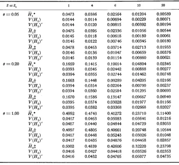
estimating mutation rate, it is better to use the number of rare alleles rather than the total number of alleles, for the former is much less affected by selection than the latter. (2) A great majority of the alleles in a sample are in low frequencies,

i.e., around or less than 0.01, and are largely due to mutations of the second or third class. (3) The n4 value is larger for case 3 than for case

2

when S, = S = 4,

but the situation is reversed when S, = S = 30. A simple explanation for this phenomenon is as follows. In case 3, only a minority of mutations, less than

2 percent, belong to the first class. Therefore, when S, = 4 there is a high probability that the first-class alleles are in very low frequencies or even absent from the population (see the first values in parentheses f o r case 3 with 6 = 0.448).

Compared with case 3, there should be more first-class alleles in case 2 because about 10 percent of the mutations belong to this class. Consequently, selection is weaker in case 3 than in case 2, so that n, is larger folr case 3 than f o r case 2. On

the other hand, when S, = S = 30, selection becomes effective, so that the sum of the frequencies of the first-class alleles is high even in case 3. Now selection is stronger in case 3 than in case 2 because more alleles are selected against, and thus n, is smaller for the former than f o r the latter.

The sampling property of allele frequencies can be used to detect the presence of selection. To see this, we consider the following example. Cases 3 with

0 = 0.448 and 6 = 3.36 are equivalent to the cases of 4N = 4

x

lo5 and

4N

=

3

x

IO6 in Figure 2, respectively. As noted earlier, the mean heterozygosities for these two cases are virtually equal: 0.268 and 0.269. If we assume that the heterozygosity of a population is completely due to neutral mutations and use = 0.270

to estimate 6, then we get 6 = 0.37. The values of n, for neutral mutations with 6 = 0.37 are given in the last column of Table 2. It is clear that the differences in these values between the cases of genic selection and neutral mutations are negligibly small if S, = 4 and S, = 2, but very large if S, = 30 and Sz = 15. In particular, no.ol for the case of genic selection with S1 = 30 and S, = 15 can be more than eight or nine times that for neutral mutations. We shall discuss the implication of this finding for protein polymorphism later.

MEAN A N D VARIANCE O F HETEROZYGOSITY

Let

H

and J denote the heterozygosity and hofmozygosity o'f a locus. Under random mating,

J = X 1 2 + . .

.

+

x K 2

,

so that

K hi K

The variance of

.I

is given by V ( J ) = E(],)

- F .

Since H = 1

-

J,

B

= 1

-7

(20)

368

the moments of

1.

When there is no selection, the following results agree with

those for the case of neutral mutations obtained by KIMURA and CROW (1964),

STEWART (1976)

,

WATTERSON (1974) and

LJ

and NEI (1975).

Genic Selection

by folrmula (3') and

In the general case, the joint probability density of gene frequencies is given

E(]) =

c

J

. .

.

J

5

zi2+(z1,.

.

,zL)dxl..

.

dzL R %=1

2 N n!2"

E ( P ) = C I: ('")

n=O n

In the case olf three classes of alleles, it is simpler to derive

7

from the distri-

E(]) = J:z2~(z)dx

bution of allele frequencies given by formula (14).

2 N n!2" 1

=(l+Cu) I:

( Y )

I:-

r ( n

+

2

+

0.) (n) nl!n2!

n=o

x

[ elClt2nlt3nz

r

(n,

+

e,)

r

( n2

+

e,)

+

132Cz~ln1r3n~

x r ( n ,

+

e,)r(n,

+

e,)

+

e 3 C 3 ~ 1 n l ~ 2 n ~ r ( n ,

+

e , ) r ( n ,

+

&>I,

(29)

in which the Ci's are the same as those in formula (14). To compute E(]'),

we notice that

E(],) = ZE(z14)

4-

ME(xI,4,)

4-

Q E ( ~ K ~ )

+

Z(Z - l ) E ( ~ t z i )

+

M ( M - l ) E ( ~ ~ + 2 , ~ ~ + 2 ~ )

+

Q(Q - 1)E(z2,~;)

+

2ZM E(z;zr,2,)

+

2ZQE(z:z:)

+

2MQE(x1,2,x;).

From the joint distribution of zl,.

. .

,~1-1,y2, and y 3 given by formula (8)

(21)

From formulae (IO) and (12), we obtain

E(z;z;) = a 2 ( a

+

l)2E(z;)/(a)4.

To evaluate E(X~X,,"~), we consider the joint distribution of xl,

zl,

z l + ~ , and y 3 , where z1 = yl - zl, and find that

. . .

,

+ ( ~ ~ , z ~ , z I + ~ ,

. . .

,xI+M-l,yS) =

C 4 r ( p q

1

+

2rlxl

+

2rlzl

+

27-&~3)'~

n!2" rln~r3n~rln3

ZN

c-1

= ( 2 N )

z

r ( n l

+

e,-

r ( n

+

e.)

n1!n2!n3!

4 n=o

n!2" SlnISznzSln3

r ( n + 0') ( n ) n1!n2!n3!

2 N

?=

z

(")

z

r ( n l

+

e,

-

a ) r ( n ,

+

e2)r(n3

+

a),

n=o

(22)

x r ( n , + ~ , ) r ( n , + e , - ~ ) r ( n , + 2 + ~ ) , n!2" S1n1Szns2n3

2 N

c-1

(")

z

r ( n l

+

s,)r(n,

+

e,

- 4

r ( n

+

e')

( n ) nl!n,!n,!

6 n=o n

x r ( n ,

+,.I,

where zz = y 2

-

zr+,.

By using these results, E(J2) can be obtained. In the case

of infinite alleles, it becomes

E(J2) = ZN (") n!2"

- z -

[81(6

+

e1)clt2nlt3n2 R=O n r ( n + 4 +

e )

( n ) n,!n2!

+

e l e 3 ~ 3 ~ l n l + n ~ S 2 ~ 2 r ( n l

+

e,>r

(n2

+

e,)

+

e 2 e 3 c 3 ~ 1 n 1 ~ 2 n z + n 3

x r ( n l

+

e m n ,

+

e2)i,

(30)

because

I

C, + 01C2,

I

C5 -+ O1C,, and

M

c6-+ B,C, as

K

-+

The corresponding formulae for the case of two classes of alleles are 2 N

n=o

E(]) := ( I + a )

z

(","2n[e,~,tnr(n

+

e,)

+

e2Czsnr(n

+

e,)]/r(n

+

2

+

e')

,

(31

1

r ( n ,

+

e,)

I. (32)

+

O z ( 6

+

e2)c2snr(n+

e,)

+

2 e l e z c z ~ ~

x

~

n,+ 1

( n ) n,!

where C , and C , are given in formula (16). Note that formula (32) is written under the condition of

K

= m, but formula (31) holds for any K .

Recessive selection

formula ( 2 3 ) . The formulae corresponding to (31) and (32) are

(23)

in which the last summation

negative integers such that nl

+

n, = 2n.

Numerical examples

( A ) Mean heterozygosity: Table 3 shows the mean heterozygosity of a population under various types of selectioa. The parameters are specified in the table and the footnotes of the table. In all cases, the model of infinite alleles is used. The mean heterozygosity for the case of overdominant selection is computed by numerical integration of formula ( 2 5 ) , while those for the other cases are computed by using the above formulae. The case of neutral mutations is given for comparison. A number of interesting properties are observed. (1) Overdominant selection increases considerably the amount of mean heterozygosity, even if the heterozygote advantage is as tiny as 10-5. (2) In large populations, the mean heterozygosities for the cases of genic and recessive selection are much less than those for the case of neutral mutations. Thus, in large populations even slight purifying selection causes a great reduction in heterozygosity. This is particularly so in the cases of genic selection and confirms OHTA and KIMURA’S (1975) result by simulation. (3) The

H

value for the case of neutral mutations is somewhat

z

is over all vectors ( 2 n ) = (n,,n,) of non-

( z n )

TABLE 3

Mean heterozygosity under various types of selection

4N 4x104 106 2x106 4x105 10’ 2x10’ 3X10e 4x10’

0 =4Nv 0.04 0.1 0.2 0.4 1 2 3 4

Neutral mutations 0.0385 0,0909 0.167 0.286 0.500 0.667 0.750 0.800 Overdominant selection* 0.0405 0.1038 0.208 0.384 0.636 0.765 0.820 0.850 Recessive selection?:

Case 1 0.0389 0.0928 0.168 0.257 0.354 0.435 0.489 0.541 Case 2 0.0385 0,0911 0.167 0.273 0.322 0.360 0.380 0.398

Case 1 (2 classes) 0.0383 0.0893 0.153 0.208 0 . M 0.308 0.361 0.407 Case 2 (2 classes) 0.0385 0.0907 0.165 0.259 0.207 0.204 0.212 0.219 Case 3 (3 classes) 0.0384 0.0904 0.163 0.253 0.237 0.220 0.227 0.234

* The heterozygote and homozygote fitnesses are 1 and 1 - s, where s = 10-5. -I. Case 1: e, = O.le, e, = 0.9e, s = 10-5; Case 2: el = 0.01e, e, = 0.99e, s = 10-5.

$Case 1: e, = O.le, e, = O.9e, s = 10-5; Case 2: e, = 0.01e, e, = 0.99e, s = I W ; Case 3:

Genic selection$:

(24)

smaller than those for the cases of recessive selection if 4N is about 2

x

IO5 or less. This seems peculiar but may be explained as follows. If mutations are neutral and

N

is small or intermediate, there is a high probability that the popu-

lation is monomorphic at the time of observation. In the case of recessive selection, on the other hand, there exists some sort of mutation-selection balance because unfavorable mutations are only slightly selected against, and they occur more often than favorable mutations. This balance reduces slightly the probability of being monomorphic (see LI 1977) and, consequently, increases the mean heterozygosity to a small extent. As an example, when 4N = IO5, (P(O.99) is 6.373 for the case of neutral mutations, but 6.339 for the case of recessive selection with O1 = 0.1 O (case 1). Note that this balance is strongly affected by random drift, so that there is a high probability that the first-class alleles will become very rare or even absent from the population, if the proportion of favorable mutations is very small, say 1

%

or less. This explains why the value for the second case of recessive selection is very close to that for the case of neutral mutations, if 4N is about 2 X IO5 or less. This also explains why

@

is larger for the second case of recessive selection than for the first case of recessive selection when

4N

is around

4

X IO5. However, as the population size increases, the

a

value for the second case becomes smaller than that for the first case, because selection becomes effective and the proportion of unfavorable mutations is larger in the second case than in the first case. (4) I n the cases of recessive selection and the first case of genic selection, increases with increasing

N ,

but in the second and third cases of genic selection first increases, then decreases and then increases again as

N

increases.

(25)

TABLE 4

Mean heterozygosity under genic selection when there are I optimal states

4N 4x104 2x105 4X105 10'' 2x108 3 x 1 0 " 03

Two classes* I = I 0.0388 0.166 0.260 0.202 0.190 0.190 0.190

I = 2 0.0392 0.165 0.246 0.204 0.205 0.212 0.595

I = 10 0.0420 0.167 0.225 0.254 0.309 0.356 0.919 Three classesl. I = 1 0.0388 0.164 0.255 0.236 0.208 0.208 0.208

I = 2 0.0391 0.164 0.246 0.230 0.223 0.230 0.604

I = 10 0.0420 0.167 0.232 0.270 0.323 0.369 0.921

~ ~~

* Two classes: s = 10-5, the mutation rate to slightly deleterious alleles is 10-6, and the muta- tion rate to an optimal state is IW.

f Three classes: s, = 10-5, sz = 0.5

x

10-5, the mutation rate to the third class of alleles is 0.9

x

10-6, the mutation rate to the second class is 0.1

x

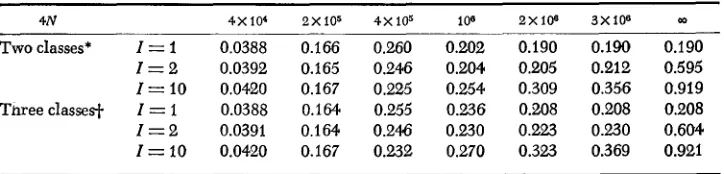
10-6, and the mutation rate to an optimal state is 10-8.

Table 4 shows the mean heterozygosity for the case where the number, I , of the first-class allelic states is small rather than infinite. The first-class alleles are called the optimal alleles. In all cases the mutation rate from all other alleles to an optimal allele is 1 O-s. In the case of two classes of alleles, the number of allelic states of the second class is infinite with uz =

1W6.

In the case of three classes of alleles, the numbers of the second- and third-class allelic states are infinite with

uz = IO-' and u3 = 9 x lo-'. The mean heteroeygosity for

N

= is computed by

using a deterministic model. Namely, in the case of two classes of alleles, the sum of the equilibrium frequencies of the second-class alleles is Q = uz/s =

low5

= 0.1, and the alleles of this class do not contribute to homozygosity. The frequency of an optimal allele is (1 - q)/Z, so that the homozygosity of the population is

f=

I [

(1

-

q )

/I]

= (1

-

q ) 2 / Z and the heterozygosity is = 1

-

7.

The heterozygosity for the case of three classes of alleles for

N

= 00 is computed

in a similar manner. It is seen that, if I = 1, the mean heterozygosity reaches the deterministic value when 4Ns is 20 or larger. This means that the effect of random genetic drift is negligible when 4Ns is of this order of magnitude. On

the

other hand, if I 2 2, the mean heterozygosity is still far from the deterministic value, even if 4 N s = 3 0 . This is because the optimal alleles are neutral with respect to each other and their frequencies are much affected by random genetic drift. Note that in the two cases of I = 10, always increases with increasing

N ,

while in the other four cases first increases, then decreases and then increases again. The explanation is similar to that given above.

( B )

Mean heterozygosity for many classes of mutations: So far we have con-

(26)

3

limited number of classes, as pointed out earlier. Thus, in order to get some idea about the mean heterozygosity f o r the continuous case, we must make some simplifications. W e consider only genic selection. Let the relative fitness of the best genotype be 1 and let s be the selection coefficient against any particular mutation. I t is clear from the above computations that genic selection causes a great reduction in mean heterozygosity when s is considerably larger than 1/N (see Tables 3 and 4). We therefore consider only mutations with selection coefficient of 0 5 s i 1 / N . Assume that 6 = 4Nv = 0.1. We first make a n effort to see how fast the mean heterozygosity for the discrete case approaches the value for the continuous case as the number of classes increases. To this end, we use a simple model in which the selection coefficient of mutations is uniformly dis- tributed over the interval [O,l/N]. If mutations are not divided into classes and are assumed to be equally fit (neutral), then

H =

O / ( l

4-

6) =0.091. Next, we approximate the continuous model by a model of two equal classes of mutations with 6, = O2 = 6/2.

It

is easily computed that the mean selection coefficient against the first-class alleles is 1/(4N) and that against the second-class alleles is 3/(4N). If we assume that the relative mean selection coefficient against the first-class alleles is 0, then that against the second-class alleles is 1/(2N). Putting these parameters into formula (31), we obtain p=O.O815. Third, we approximate the continuous model by a model of three classes of mutations with = O2 = 6, = 8 / 3 . It is again easily computed that the relative mean selection coefficients against the first-, second- and third-class alleles are 0, 1/(3N) and 2 / ( 3 N ) . Using formula (29)

,

we obtain

fi

= 0.0796. For the models of four and five classes of mutations, we obtain

B

= 0.0789 and

fl=

0.0786, respectively. These results suggest that the mean heterozygosities for the discrete models quickly approach a limit as the number of classes increases-the limit must be larger than 0.0779, the value for the first of the two models given below. Since the difference between 0.0786 and 0.0779 is small, we consider the model of five classes of alleles a good approximation to the continuous model. W e now consider another two models of five classes of mutations. In the first model, 8, = 6/15, 02=26/15,

. . .

,

8,=50/15, and the selection coefficients against the five classes are 0, 1/(5N),

.

,4/(5N). The mean heterozygosity for this model is

B

= 0.0779. In the second model, 6, = 56/15, 6 2 = 46/15,

. . .

,

d 5 = 8/15, and the selection coefficients are again 0, l / ( 5 N ) ,

.

. .

,4/(5N). The mean heterozygosity for this model is

i?

= 0.0827. Thus the value is somewhat larger for the case where the distribution of s is skewed toward 0 than for the case where the distribution of s is skewed toward 1/N. I n all cases, however, the values are at most 15 percent less than 0.091, the value for the model of strictly neutral mutations with B = 0.1. We note that the prevalent mode of selection in nature is probably less effective than genic selection. We may therefore conclude that, regardless of what the fitness spectrum of mutations may be, all mutations with