THE DYNAMICS OF FINITE HAPLOID POPULATIONS WITH OVERLAPPING GENERATIONS. II. THE DIFFUSION APPROXIMATION

THE DYNAMICS OF FINITE HAPLOID POPULATIONS

WITH

OVERLAPPING GENERATIONS.

11. THE

DIFFUSION

APPROXIMATION1

TED H. EMIGH

Department of Statistics, Iowa State University, Ames, Iowa 50011

Present address: Department of Statistics, University of Georgia, Aihens, Georgia 30602

Manuscript received November 15,1977 Revised copy received September 22, 1978

ABSTRACT

The dynamics of a gene in a haploid population can be explained approxi- mately by considering the average reproductive value of the gene. The dynamics of the average reproductive value are similar to those of a gene in a population with nonoverlapping generations with the following modifications: The effective population size, N e , replaces N ; the average mutation rates ,u* and v* replace fi and Y ; the average overall selection r*+(T-l)s** replaces

s; and time is measured in terms of generations, T. The implications of the average selection coefficient to adaptive life histones are discussed.

HE model and moments for a haploid population with olverlapping genera- tions is introduced in the first paper of this series (EMIGH 1979). Of special interest is that lim Vij ( t )

-

V ,

which suggests that, if t is large, the multivariate process can be considered as a univariate process. Since the probability of a fixa- tion of a neutral gene is equal to the initial average reproductive value of that gene, it seems reasonable to use the average reproductive value as a summary of the population.

t+ m

MODEL FOR H A P L O I D POPULATIONS

The model we use

for

haploid populations was first introduced by

FELSENSTEIN

(1971) and extended by

EMIGH

(1976,1979). The number of haploid individuals in each age group

(i

= 1,

.

.

.

,

k)

is constant over time ( t = 0, 1,

.

.

.) and is equal to N ( i ) . We consider two genes, A , and

A,, at a locus and let

pi and v i be the mutation rates from

A,

to A , and A, to A,, respectively, for parents in age group

i.

If we let X

(i,t)

be the gene frequency of gene A , in age group

i

at time t, then the number of newborn individuals at time t

+

1 is distributed as a binomial distri- bution with parameters N ( 1) and

(1 + T i )

x

(i,t)

i 1+ri X ( i , t )

PJt+l) = Y *

+

Z&(l - p i - Vi)

340 T. H. EMIGH

with

v* = s p i v ;

-

-

average mutation rate, r = (rl,.

. . ,

r k ) ‘

ri = fertility selection coefficients of gene A I over A z .

Aging is accomplished through the noncentral hypergeometric distribution with noncentrality parameters {si} (see EMIGH 1979 for an explanation of the noncentral hypergeometric distribution). The probability of a newborn indi- vidual surviving to age group i is li =

N ( i ) / N

( 1 ) .

The effective population number for this type of population is given by (

FELSENSTEIN

1971 ; EMIGH 1979)

and

with

and

qi = J+ p j =

li

* reproducive value

T

= generation time =

3

ipi =

+

qi

1

Moments of change in gene frequencies

Assume that the frequencies of gene A , in the population at time t in the various age p u p s are x =

(xl,

.

.

. ,

xk)j. In the next time period, the gene fre- quencies will be x

+

Sx, where Sx =

(Sx,,

. .

.

,Sxk)‘ is a random variable, depen- dent on the vector of frequencies x.

The first two moments of the changes in gene frequencies, ax, conditional on the vector of frequencies, x, are obtained to order 0 ( 1/Ne2) from EMIGH ( 1979) as

and

E [ S X i I X ] =xi’-xi

,

i = l , .

. .

,k,

(1)

cov [ h i , SZjlX]

= O

,

i + i ,

where

xi’ v*

+

z

pj (1-pj

-

v j ) x j

+

Z pjrjxj (1-xj), i = 1 = z i - l ~ s i x i - l ( l - x i - l ) ,

i > ? ,

and v*=?ppivj

*

.

The third and fourth central moments are O ( 1 / N e 2 ) (see EMIGH 1976).

The diflusion approximatioln

HAPLOID OVERLAPPING GENERATIONS I1

341

not affect the approximation. The discrete changes in xi can then be approxi- mated by a continuous random variable. We also rescale the time parameter by d i v i d q by

N I T ,

where

N e is

the effective population number, and

T =

ipr,

the average age at reproduction, is the generation time. That is, in the rescaled time, the smallest difference

in

time is S t =

( I / N , T ) .

Therefore,

and

where

and

%

E ( S X i ) = m4(x) st

+

0 ( S t 2 ) ,

COV(SXi, S X j ) = U i j ( X ) S t

+

0(W),

mi (x) = (xi' - xi)

NeT,

(3)

= O

,

i # j .

The Kolmogorov Forward Equation (also called the Fokker-Planck Equation) is

with the probability density function of the vector of gene frequencies at time t

denoted b y f ( x ; t )

.

This can be rewritten as

In EMIGH ( 1 979)

,

it was shown that the covariances of gene frequencies are approximately the same. This suggests that the population can be described by

considering a summary quantity. Consider J: ( t ) =

-

qi

X (

i,t)

,

the average

reproductive value of gene A, at time t. Assuming that

{n}

rind {si} are small, the conditional mean of z ( t

+

1

) i s

I

E [ x ( t + l )

I

X ( t ) ] = -

z

qi

E [ X ( i , t + l )

I

X ( t ) ]

T i

=

-

{v'

+

3

pi(I--yi--vi)

X ( i ,

t )

+ ?

piri

X ( i ,

t )

[ I - X ( i ,

t ) ]

+

,E qi [ ( I + s i )

X(i-I,t)-si X 2 ( i - l , t ) ] } .

1 T i

1

T 2.

342 T. H. EMIGH

For t large, the X ( i , t ) ’ s are highly correlated with the same mean and vari- ance, so they may be approximated as being the same. Heme, X ( i , t ) = x ( t ) . Then,

1

E [ x ( t + l )

1

x ( t ) ] =- { v *

+

( l - p * - v * ) x ( t )

+

r * x ( t ) [ l - x ( t ) ]

{ Y *

+

(T-p* -Y

*

) x ( t )

+

(I*

+

( T - 1 ) S *

*

) T

1

T

+

( T - l ) x ( t )

+

( T - l ) s * * x ( t ) [ 1 - ~ ( t ) ] }

_ _

-

‘ x ( t ) [ 1 - x ( t ) ] } , (6)

where

V * =

p* =

p Z v Z = average mutation rate from A, to A ,

p z p L = average mutation rate from A , to A , z

r* = p i r i = average fertility rate

L

and

qisi = average viability rate (averaged by reproductive

1 s * * - _-

__

T-1 i > l

value).

The conditional variance of z ( t + l ) is found in a similar manner Var[x(t+l)

I

X ( t ) ] =

-

1

z

qtqj C o v [ X ( i , t f l ) , X ( j , t + l )

I

X ( t ) ]

T2 i j

X ( i - l , t ) [ l - X ( i - l , t ) ]

[

1 - 1

I}

P ( t + l ) ( 1 - P J t f l ) )

+

z

q 2

& - {

1

TZ N ( 1 ) i > l i N ( 1 ) li li-,

Replacing X (i,t) by

x

( t )

,

ignoring terms of

0

( 1 / N e 2 )

,

and simplifying, we obtain

Therefore, the forward equation can be approximated by weighting by the repro- ductive values and is

a

a t

ax

af(x;t) = -

-

{ m ( x ) f ( x ; t ) ]

where

m ( x ) = { v * ( l - x ) - p*x+(r*+(T-l)s**)x(l-x)} N e

,

and (9)

u ( 5 ) = x ( l - x ) .

m(d) ( x ) = ( ~ ( 1 - X )

-

For a population with discrete generations,

with the variance of gene change the same as (9).

+

s X( l - ~ ) } N , _{( 1 0 )}

1

Thus, the average reproductive value of a gene in the population, x ( t ) =

-

Z

H A P L O I D OVERLAPPING GENERATIONS I1 343 qi

X ( i , t )

,

can be analyzed in the same manner as the gene frequency in a popu- lation with discrete generations with the following changes: (1) The effective population size, Ne, replaces the population number, N ; (2) The average muta- tion rates p* and Y* replace the mutation rates p and V ; (3) An average selection coefficient, r*

+

(T-I)s**,

replaces the selection coefficient, s; and

(4)

Time is measured in generations,

T

=

7

ipi.

Before we consider the differential equation (8) in depth, it should be men- tioned that, in assuming that x can be approximately described by a single ran- dom variable z, we have assumed that t is large; i.e., the population has been reproducing for a long time. This would seem to say that this diffusion equation cannot be used to answer, for example, the question of how long a single mutant gene will stay in the population, given that it is eventually lost. On the other hand, it can help to answer questions about a population that has been going for some time. The problem of how long it will take before s ( t ) approximates

X

( t ) is considered in the next section. Average reproductive value

In the first paper of this series (EMIGH 1979), it was assumed that, after some time, the multivariate process describing a population with overlapping genera- tions can be described sufficiently well by a univariate process. The means of the age classes very quickly become approximately the same, but the covariances, V i j ( t ) , take some time. In this section, the assumplion V i j ( t ) V(t)+V for large t is explored, both to test its validity and to examine holw long this takes. This result can be seen iiituitively by considering the process of reproduction. The newborn individuals are, in a sense, the average of the individuals already present in the populatim, weighted by the pi’s. One age class, the eldest, is then eliminated, and this averaging occws again. The next average will be close to the first, but not exactly in as much as the weights for the individuals have changed

(e.g., from p z to pi+l for an individual originally in age class

i )

.

To illustrate the manner in which this homogenizing process works, define the standard deviation of the variances at time t to be

Z

where

is an average value for the variances. Equation (12) is the variance of

z ( t ) .

Therefore, u,(t) gives a measure of how far each V , j ( t ) is from the average covariance. Folr practical purposes, we can consider that most covariances are in the internal

(p

( t ) - 2 U, ( t )

,

( t )

+

2 uV ( t ) )

.

Therefore, as uV ( t ) decreases with time, the covariances become more homogeneous.

It was quickly discovered that the behavior of U,( t ) depends only upon z (0)

,

T. H. EMIGH

100 200 300 40 500 600 700 SO0 sb0 1000

Number of Generations

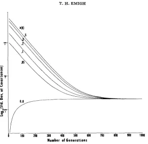
FIGURE 1.-Log,, of standard deviation of covariances with N e = 91.2 for various values of

z(O), using the first population structurein EMIGH (1979, Table I).

In Figure 1, values of loglo(crv(t)) are plotted against t, in generations, for various values of x ( 0 ) for the first population given in

EMIGH

(1979, Table 1). In this population, there are ten age classes, and the effective population size is

Ne = 91.2. The standard deviation of the covariances is less than 5 X 1 Ow3 after ten generations in the worst case ( x ( 0 ) = 0.5), so that most covariances are within of v ( t ) after only ten generations. The width of this interval decreases exponentially until generation 300 and reaches a constant value of after generation 800.

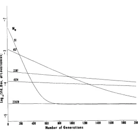
A comparison of the rate of decrease of u v ( t ) for various population sizes is given in Figure 2. For this comparison, the value for x ( 0 ) is set at

0.5,

the “worst” case from Figure 1. It is evident that the covariances become homogeneous quite rapidly, although the rate decreases for large N e . It can also be seen that a ten- fold increase in N , (from 45 7 to 45 74) decreases the initial value of U* ( t ) by ten times (from to IO-.). Hence, it seems that f o r small t , u v ( t ) is proportional to I/Ne.

HAPLOID OVERLAPPING GENERATIONS I1 345

-

0 zb 400 si0 do i o i o izw i i a o 1600 1800 2000

Number of Generations

FIGURE 2.-Log,, of standard deviation of covariances with ~ ( 0 ) = 0.5 for various values of N e .

At ten generations, the process is still far away from the equilibrium values, so that the covariances become very nearly the same value and then move toward the equilibrium value; i.e., V,j ( t ) = V ( t )

+V.

The average reproductive value seems to be a very good approximation for the population as a whole after as few as ten generations.

As another way of checking the approximation, equation (8) can be used to1 obtain solutions to the questions answered directly in the previous paper, such as probability of fixation of a neutral gene without mutation and the first two moments of the stable distribution of a neutral gene

with

mutation in both directions. These topics will be covered in the following sections.

STATIONARY DISTRIBUTION

346 T . H . EMIGH

The mean and approximate variance for the stable distribution if there is no selection has been calculated [EMIGH 1979, equations ( 3 3 ) and ( 4 9 ) ] as

M ( 1 - M )

V =

1 + 2 N e ( / ~ * + ~ * ) *

The stable distribution can be obtained from ( 1 3 ) . Assume that p * , V *

>

0, then

( 1 5 ) f(x) CxZN.v'-l ( 2N,p*-1 & p . ( I . * + (T-1)8**)

where c is a constant to be found.

This distribution is closely related to the Beta distribution, which will allow the evaluation of the first two moments of the stable distribution. From the relation J,'f(x)dx = 1,

where

M ( . )

is the confluent hypergeometric function (see JOHNSON and KOTZ

1969, page 8 ) .

If we let W have a Beta distribution with parameters a! and

p ,

then

Let a=2Nev*, p=2Ne@*, and y = 2 N e ( r * + ( T - 1 ) s * * ) . Notice that

Now, E w [erw] = M(a;a+P;y), so

Therefore, the moments of the stable distribution are given by

1

8 " ) M

(a;a+P;y)

E[X"]

=

M (.cw;*u+p;y) 8,"

JOHNSON and KOTZ (1969, page 8) give the folllowing:

a(")M(a;a!+P;y) -

- M(a!+m;a+P+m;y)

,

a y m (a+@) (")

where a(") = a!(a+l) (a+2)

. . .

(a!+m-I).

The moments of the stable distribution are given by

a!(") M(a+m; a+p+m;y)

E [ X " ] =

HAPLOID OVERLAPPING GENERATIONS I1 34 7

If

=2Ne(r*

+

(T-l)s**)

<

1, then

Y 2

-+.

.

.

,

( 2 0 )

a+@ l!

(ILY+P)

(a+P+l) 2 !

a(lY+l) M(a;a+P;y) = 1

+

--

a y +

so the first two moments of the stable distribution are

and

1 CY(a+l)

E [ X 2 ] =-

M (a;a+P;y)

[

('a+@) ( a f J 3 f l )

-+...

y

l

a ( a + l ) (a+2)

(a+P> (a+P+l) ('lYf/3+2) l !

+

-

.

v* 2Nev

*

+

1

--

p*+v*

I

2Ne(p*+v*)+1

V*

-

,&L*+V

- 4 1

*

If there is no selection, r*

+

(T-1 ) s*

*

= 0, then the first two moments are exactly

V*

M = E [XI =-

p*+v*

,

and

) 7 so that

M ( 1 - M ) 1+2Ne ( P * + v * )

'

Var(X) =

which is as we calculated the stable distribution mean and variance directly, equation (14). These values have been calculated for neutral genes with discrete generations by WRIGHT ( 193 7 ) .

The Kolmogorou backward equation

Using m

(x)

and U (z)

,

from ( 9 )

,

the Kolmogorov backward equation is

W X P ( O ) , t )

W O )

a f ( x ; x ( o ) 7 t ) = N e [ V * ( 1-x) -p*z+ (r*

4-

( T- 1 ) s*

*

)

x

( 1

-x)

]

at

where f ( x ; x(O), t ) i s the probability density of the average reproductive value,

x,

at time t given that it had the value x ( 0 ) at time S O .

348 T. H. EMIGH

becomes fixed, given initial reproductive value z (0). Then, from KIMURA (1962),

where

G ( x ) =exp [-2 S d y ] .

U (Y)

Using the values for m ( y) and U ( y) this becomes

l-exp {-2Ne (r*+(T-l)s**) z(0))

u ( z ( o ) ) = l-exp {-2Ne (r*+(T-l)s**)) 7 (27) which is approximately

If I*

+

(T-1 ) s*

*

= 0, this becomes exactly

the initial reproductive value. This latter is the value found in the previous paper (EMIGH 1979, equation (27)), and

both

are extensions of the discrete generations results.

The backward equation also can be used to find the mean time to fixation given that the gene is eventually fixed (see KIMURA and OHTA 1969). The time to fixation, given fixation, is

u ( z ( 0 ) ) = z(0)

+ N e (r*+(T-l)s**)

z(0) [l-z(O)]. (28)

u ( z ( 0 ) )

= d o ) ,

(29)

t,

( d o ) )

= { u ( z ( O ) )

J:(o)m

U([> [l-u(t>I dt

+

[1-u(dO))l

q4.9

u ( t ) 2 dt)/u(z(O)), (30) where

2

s’,

G(5) dt ‘(z) = u ( z ) G ( x )

’

and G ( x ) is from (26).

Letting S =

N,(r*

+

(T-l)s**), it is easy to obtain (KIMURA and OHTA 1969)

Of

special interest is the mean time to fixation of a selectively neutral mutant

1

gene, initially in the new born age group. Then, x ( 0 ) = ___

HAPLOID OVERLAPPING GENERATIONS I1 34.9 and

= 2N, ( 3 3 )

for large N ( 1 ) T .

It

should be noted that with this starting value, x ( 0 )

X(i,O)

for all

i

except

i =

l.Hence, it may be expected that the diffusion will give reasonable results.

DISCUSSION

As

FISHER

(1930) surmised, a population with overlapping generations can

be approximately described using the average reproductive value of the popu- lation.

If

U $ is the reproductive value of age group

i,

then vi = q;/li. The average reproductive value of gene A , is s ( t ) =

-

Zuil$X(i,t).

The average reproductive value is a good summary for the complex reproduc-

tion and survival structure associated with a population having overlapping generations. In less than ten generations, the average reproductive value does quite well. However, events that would normally occur in this time, such as time to loss of a single mutant gene, may not be adequately answered through the use of x ( t ) .

Using x ( t ) , the population can be adequately described in analogy to a popu- lation with discrete generations with the following parameter changes: the population size becomes the effective population size, Ne, as given by FELSEN-

STEIN (1971; see

EMIGH

1979, equation 4); the mutation rates become ,U* and

v * , average mutation rates of A , to A, and A , to A,, respectively; time is measured in generations, T ; and the selection coefficient becomes the average selection coefficient I*

+

(T-l)s**, where I* is the average fertility selection coefficiens

and s** is the average selection coefficient of surviving from one age to the next (averaged by reproductive values).

I n reference to the seleciion coefficient, I*

+

(T-I)s**, it is easily seen that,

for organisms with long generation times (T large) the viability selection has a much larger effect than for organisms with short generation times. Although we may expect that average viability selection from one age to the next is smaller than average €ertility selection, s**

<

r*, if T is large, the effect of viability selec- tion on the population may be larger than the effect of fertility selection. On the other hand, if

T

is small, then it would be expected that fertility selection has the greater effect on the population. Since the viability coefficients si, are averaged with respect to qi, which is a nonincreasing function of age, it means that differential viability is more pronounced in very young individuals, or most probably, operates through the difference in the average number of individuals surviving to reproduction.

The evolutionary significance of this is obvious. If an individual in a popula- tion with a long generation time is able to increase its viability prior to repro- duction then it will have a selective advantage, even at the cost of lowered sur-

350 T. H. EMIGH

viva1 after mean age of reproduction or lower fertility during reproduction. There is a very large literature on adaptive strategies in life histories, starting with MEDAWAR (1952, 1957) and COLE (1954). Three of the theories covering evolution of senscence are: (1) Group selection ( WYNNE-EDWARDS 1962)

,

which proposes that individuals die to help the species; (2) Individual selection (WILLIAMS 1957), which proposes specific genes which lower an individual s

fitness at older ages; and (3) Selective irrelevance (MEDAWAR 1952, 1957), which proposes that genes whose effects do not appear until old age would not be selected against since, even with nonsenesent individuals, the selection pressure is very slight.

The present paper allows for a mechanism of individual selection in a popu-

lation that has a stable population size. The average selection coefficient, s = r*

4-

(T-l)s**, is a measure of the selection f o r senescent genes, and can be used to compare various life history strategies. Most genes have many effects on the organism, either directly or indirectly. Thus, a single mutation may have positive effects for some aspects of the organism and negative effects for other aspects of the organism. One simplistic way of looking at this is through resource (or energy) allocation (cf., GUTHRIE 1969, L E ~ N 1976,

PIANKA

1976 or CALOW 1977). For example, a mutation which allows more of an individual’s resources to go into muscle production may allow relatively fewer resources to go into muscle repair. Then, si

>

0 for small

i

and si

<

0 for large

i.

This mutation will

be selected if s**

>

0, which is likely since si is given a larger weight for small

i

than for large

i.

Although this model assumes a haploid population, the extension of this to diploid populations does not seem too great. Effective population numbers have been calculated by

JOHNSON

(1977b) under the assumption of random mating of all individuals and more generally by

JOHNSON

(1977a) and

EMIGH

and

POLLAK (1979) under the assumption of random mating, but with age selectivity possible. It was found that the effective population number does not differ greatly from that under a haploid population so long as the life tables of the two sexes are similar (EMIGH and POLLAK 1979). It is expected that the same results will hold for the specific dynamics of diploid populations and will be considered in a further paper.

Portions of this paper appeared in m y thesis (EMIGH 1976) under the direction of OSCAR KEMPTHORNE. I greatly appreciate his guidance, Helpful comments and suggestions by EDWARD POLLAX regarding the thesis and this paper also are appreciated. Comments on an earlier draft of the paper by JOSEPH FELSENSTEIN and an anonymous reviewer are gratefully acknowledged.

LITERATURE CITED

CALOW, P., 1977 Ecology, evolution and energetics: A study in metabolic adaptation. Adv. Ecol. Res. 10: 1-62.

COLE, L. C., 1954 The populations consequences of life history phenomena. Quart. Rev. Biol.

2 9 : 103-139.

H A P L O I D O V E R L A P P I N G G E N E R A T I O N S I1 351 of finite haploid populations with overlapping generations: I. Moments, fiiation probabili- ties and stationary distributions. Genetics 92 : 323-337.

EMIGH, T. H. and E. POLLAK, 1979 Fixation probabilities and effective population numbers in diploid populations with overlapping generations. Theor. Popul. Biol.

FELSENSTEIN, J., 1971 Inbreeding and variance effective numbers in populations with over- lapping generations. Genetics 68: 581497.

FISHER, R. A., 1930 The Genetical Theory of Natural Selection. Oxford University Press, Oxford.

GUTHRIE, R. D., 1969 Senescence as a n adaptive trait. Persp. Biol. Med. 12: 313-324.

JOHNSON, D. L., 1977a Inbreeding in populations with overlapping generations. Genetics 87 :

581-591. -, 1977b Variance-covariance structure of group means with overlapping generations. pp. 851-858. In: Proc. Int. Conf. on Quant. Genet. Edited by E. POLLAH, 0.

KEMPTHORNE and T. B. BAILEY, JR., Iowa State Univ. Press, Ames.

JOHNSON, N. L. and S. KOTZ, 1969 Distributions in Statistics: Discrete Distributions. Houghton Mifllin Co., Boston.

KIMURA, M., 1962 On the probability of fixation of mutant genes in a population. Genetics

47: 713-719.

KIMURA, M. and T. OHTA, 1969 The average number of generations until fixation of a mutant gene in a finite population. Genetics 47: 713-719.

L E ~ N , J. A., 1976 Life histories as adaptive strategies. J. Theor. Biol. 60: 301-335.

MEDAWAR, P .B., 1952 A n Unresolved Problem in Biology. H. K. Lewis, London. -

,

1957

PIANHA, E. R., 1976 Natural selection of optimal reproductive tactics. Am. Zoologist 16:

WILLIAMS, G. C., 1957 Pleiotropy, natural selection, and the evolution of senescence. Evolution 11: 398411.

WRIGHT, S., 1937 The distribution of gene frequencies in populations. Proc. Natl. Acad. Sci., U.S. 23: 307-320.

-

, 1945 The differential equation of the distribution of gene frequencies. Proc. Natl. Acad. Sci. U.S. 31: 382-389.

WYNNE-EDWARDS, V. C., 1962 Animal Dispersion. Hafner, New York. The Uniqueness of the Individual. Basic Books, New York.

775-784.