This dissertation research embodies projects about crop insurance programs that has attracted a lot of attention as far as food and agricultural policies in the United States are concerned.
To this end, this dissertation tackles several dimensions of crop insurance, yielding findings that are important for the design of crop insurance products and policy. More importantly, this dissertation extends the literature on crop insurance in three distinct ways.
In the first paper, a Bayesian nonparametric model which is based on Dirichlet processes for yield estimation is proposed. The framework is deployed for the empirical estimation of county
level yield data for cotton from the continental United States. We then examine the implications of our modeling framework on the pricing of the Group Risk Plan (GRP) insurance compared to a nonparametric Kernel-type model. The empirical analysis suggest that our proposed model
provides slightly higher insurance premium rates.
There is mounting evidence about how price sensitive producers in the United States are
to participate in crop insurance, generally suggesting a wide range of elasticities. Most of the previous literature fail to address the endogeneity of insurance premiums. The second paper addresses this challenge and attempt to provide well-identified elasticity estimates that reflect
current state of the world of the Federal crop insurance program, using a variety of methods. Our preferred empirical model exploits exogenous variations from major Federal subsidy policy
yields-weather relationships. The results suggest the following. First, cooling degree days and
precipitation negatively affect yields, yielding estimates that lie within the range of those provided in previous studies. There is evidence of nonlinearities in effects, along with time-varying effects which have important implications for the timing of agricultural crop production activities
including Agricultural Extension support to farmers. One major contribution of the third paper is the systematic distinction made in terms of “When” various weather variables matter for crop
© Copyright 2017 by Yang Wang
A dissertation submitted to the Graduate Faculty of North Carolina State University
in partial fulfillment of the requirements for the degree of
Doctor of Philosophy Economics
Raleigh, North Carolina 2017
APPROVED BY:
_______________________________ _______________________________ Dr. Barry K. Goodwin Dr. Sujit K. Ghosh
Chair of Advisory Committee
DEDICATION To my parents, Mingzhe Wang and Jieyu Yang
BIOGRAPHY
Yang Wang was born in China. She received a Bachelor’s of Arts at Jilin University of Finance
ACKNOWLEDGMENTS
First, I would like to show my sincerest gratitude to my advisers, who have been top notch and a
pleasure to work with. Dr. Barry Goodwin has played a major role in developing the ideas for this work and also helped me with professional advice. He has shown enthusiasm and support throughout this process. Dr. Sujit Ghosh has been generous with his good ideas and with his time
by meeting with me. His continuous support and insightful suggestions made it much easier to accomplish this dissertation. Special thanks also to Dr. Roderick Rejesus, for his expertise on this
topic and always being willing to answer my questions; and Dr. Nicholas Piggott, for his attention to detail with my work and being a great professor of two of my courses and career advice; and Dr. Xiaoyong Zheng, for his insights and expertise on economics questions. Their insightful
comments on my research have improved this work significantly. I would like to thank my parents for their unwavering support and encouragement. I’d like to also thank my grandparents for
TABLE OF CONTENTS
LIST OF TABLES vii LIST OF FIGURES viii
1. CHAPTER 1 1
1.1. BACKGROUND 2
1.1.1. FEDERAL CROP INSURANCE PROGRAM 4
1.1.2. INSURANCE PLANS 6
1.2. MODEL AND ESTIMATION 7
1.2.1. PROBABILITY MODEL 9
1.3. DATA,INFERENCE AND VALUATION 12
1.3.1. DATA SETS 12
1.3.2. INFERENCE 13
1.3.3. INSURANCE VALUATION 14
1.4. PROOF OF CONCEPT 15
1.4.1. PROCEDURE 15
1.4.2. RESULTS 16
1.5. RESULTS AND DISCUSSION 18
1.5.1. MAIN RESULTS FOR ENTIRE UNITED STATES 18
1.5.2. THE CASE OF TEXAS AND VISUAL EVIDENCE 20
1.6. CONCLUSION 23
2. CHAPTER 2 44
2.1. INTRODUCTION 45
2.1.1. FEDERAL CROP INSURANCE PLANS 47
2.2. DATA AND MEASUREMENTS 54
2.3. MODELING AND ESTIMATES 57
2.3.1. PANEL ESTIMATES 58
2.3.2. PANEL ESTIMATES 63
2.3.3. ROBUSTNESS CHECKS 65
2.4. HETEROGENEITY IN INSURANCE DEMAND 67
2.4.1. RESULTS 68
2.5. CONCLUSIONS 72
3. CHAPTER 3 91
3.2. DATA AND SUMMARIES 94
3.3. METHODOLOGY 97
3.4. RESULTS AND DISCUSSION 101
3.4.1. WHAT AND WHEN DOES WEATHER MATTER? 101
3.4.2. TO WHAT EXTENT DOES YIELD CORRELATES YEAR-TO-YEAR? 106
LIST OF TABLES
Table 1.1 Differences in Estimates between “True” and Competing Models ... 37
Table 1.2 Cotton Belt: Estimates for 75% Coverage ... 38
Table 1.3 Cotton Belt: Estimates for 80% Coverage ... 39
Table 1.4 Cotton Belt: Estimates for 85% Coverage ... 40
Table 1.5 Cotton Belt: Estimates for 90% Coverage ... 41
Table 1.6 Actuarial Estimates under Alternative Models with 75% Coverage ... 42
Table 1.7 Robustness with Different Coverage Levels ... 43
Table 2.1Summary Statistics of “Insured Area” ... 79
Table 2.2 OLS and Panel Estimates: under Alternative Specifications ... 80
Table 2.3 Panel IV Estimates: under Alternative Models ... 81
Table 2.4 OLS and Panel Estimates-logit: under Alternative Specifications ... 82
Table 2.5 Panel IV Estimates-logit: under Alternative Models ... 83
Table 2.6 Panel IV Estimates (Subsidy Rate) ... 84
Table 2.7 Coverage Measure Elasticity Estimates under Alternative Models: OLS and Panel ... 85
Table 2.8 Coverage Measure Elasticity Estimates under Alternative Models: Panel IV ... 86
Table 2.9 Robustness Checks: Elasticity Estimates for Different Time Trends: OLS and Panel 87 Table 2.10 Panel IV Estimates Using SUR Estimation ... 88
Table 2.11Panel IV Estimates Using SUR: Robustness Checks for Different Trend Models ... 89
Table 2.12 Papke and Woodbridge Estimates: under Alternative Specifications ... 90
Table 3.1Summary Statistics of Variables ... 110
Table 3.2 What Weather Variables Matter for Yields ... 111
Table 3.3 Group LASSO: What and When Does Weather Matter for Yields ... 112
Table 3.4 Group LASSO: What and When Does Weather Matter for Yields ... 113
Table 3.5 Correlations Between Current and Past Yields ... 114
Table 3.6What and When Does Weather Matter for Yields ... 115
Table 3.7 What and When Does Weather Matter for Yields ... 116
LIST OF FIGURES
Figure 1.1Counties in Cotton Belt for the United States ... 26
Figure 1.2 Model Fit Checks Using Simulated Known Densities ... 27
Figure 1.3 QQ Distribution Plots ... 29
Figure 1.4 Counties in Texas for Cotton Production ... 30
Figure 1.5 Densities: Crosby and Dawson ... 31
Figure 1.6 Densities: Floyd and Gaines ... 32
Figure 1.7 Densities: Hale and Hockley ... 33
Figure 1.8 Densities: Lynn and Martin ... 34
Figure 1.9 Loss Probabilities: Crosby, Dawson, Floyd, and Gaines ... 35
Figure 1.10 Loss Probabilities: Hale, Hockley, Lynn, and Martin ... 36
Figure 2.1 Distribution of “Insured Area” ... 76
Figure 2.2Data Set: Corn-Counties, Average Insured Fraction ... 77
1.
Chapter 1
Bayesian Nonparametric Estimation of
Yield Distributions
Abstract
The pricing of crop insurance products depends crucially on the accurate estimation of the underlying yield densities. Multiple estimation methods have already been examined in the
literature; but the need for other potential candidates remains essential. Here, we propose and examine a Bayesian nonparametric model which is based on Dirichlet processes for yield
estimation. We deploy our proposed model for the empirical estimation of county level yield data for cotton from the continental United States. Next, we examine the implications of our modeling framework on the pricing of the Group Risk Plan (GRP) insurance compared to a nonparametric
Kernel-type model. Our analysis provides strong visual evidence that our proposed Bayesian nonparametric model estimate densities that smoothly evolve as a function of potential
checks and proof of concept indicate that the proposed model overwhelmingly outperforms the nonparametric Kernel.
1.1. Background
The statistical modeling and evaluation of densities to capture yield risks is of great importance for rating the various yield-based crop insurance products. Therefore, accurately estimating the
yield densities plays an important role for crop insurance rating. In addition, the “small” probability lower tail events within the distribution of yield outcomes trigger insurance payments. Such risky probabilities are however hard to quantify in practice due to the infrequent nature of
these lower tail events. To this end, several yield modeling approaches have been examined spanning parametric (e.g. see Sherrick et al. 2004), semi-parametric (e.g. see Ker and Coble 2003),
and nonparametric Kernel-type (e.g. see Goodwin and Ker 1998) methods. The advantages and disadvantages of the afore mentioned methods have been well discussed in the literature (e.g. see Ozaki et al. 2001).
More formally, we do not know the true underlying yield density and vis-a-vis the data generating process. An important observation is that in higher weather risk regions the yields may
exhibit an irregular pattern of yield densities.1 Irregular Distributions: These correspond to
1 Irregular Distributions: These correspond to distributions that are characterized by multiple
distributions that are characterized by multiple modes and formed from mixing multiple distributions. This may indicate several patterns of response or extreme realizations. In this case,
the distribution in the population is not simply normal or unimodal. This is in the spirt of Chen and Miranda 2008 who pointed out that certain crops (e.g., upland cotton) and regions (e.g., Texas) exhibit high post-planting abandonment rates in years of unfavorable weather. In such regions,
near zero yield realizations are likely and therefore make commonly used unimodal continuous probability distributions inadequate for modeling yield behavior and underlying uncertainty. It is
therefore important to bear this in mind when predicting yield distributions. The literature has not given much attention to these phenomena so far; but we note that this may become very crucial under current projections of climate change and amplification of climate extremes (IPCC 2012).
Here, we propose a generalized approach (i.e., a Bayesian nonparametric modeling approach) that nests this irregular phenomenon, with additional gains in accurately modeling yield distributions.
The proposed Bayesian nonparametric modeling approach is applied to an empirical context that likely exhibit irregularities in yield behavior. The overarching goal is to propose a tractable framework and illustrate how the framework can be applied to model yield distributions in general,
with special attention to irregular distributions. As we will illustrate in the empirics, the proposed approach performs well in modelling general distributions, including potential irregular patterns.
2We provide an empirical application using county level yield data for the cotton belt in continental
United States. Our approach is based on dependent Dirichlet processes, and therefore allows for
the entire distribution to smoothly evolve as a function of potential yield patterns. The full posterior inference and predictions are obtained using Markov Chain Monte Carlo MCMC. To the best of our knowledge this paper is the first to consider such formulation in the crop insurance literature.
As a companion to our empirical analyses, we examine the implications of our modeling framework on the pricing of county-based (the Group Risk Plan GRP) crop insurance contract
compared to a nonparametric Kernel-type model. Since our Bayesian approach is nonparametric, the natural candidate model is the Kernel.
1.1.1. Federal Crop Insurance Program
The United States Federal Crop Insurance Program (FCIP) has gained tremendous momentum as far as the United States food and agricultural policies or programs are concerned. The program
was created in the 1930s as a risk management tool and has now become one of the major agricultural support programs in the United States. The coverage of the FCIP was initially limited but is currently characterized by a mix of many programs.
2 As we will illustrate in the empirics, the proposed approach performs well in modelling general
The crop insurance programs have undergone many modifications through the passage of various federal Acts and farm bills, which are discussed below. 3The enactment of the 1980 Federal
Crop Insurance Act significantly expanded crop insurance to many more crops and regions in the country. The Act greatly encouraged participation by offering farmers subsidized insurance premiums. Between 1988 and 1994, annual ad hoc disaster assistance programs were implemented
to further provide relief to producers. Notably, the 1994 “Crop Insurance Reform Act” eliminated annual disaster programs, and made participation in crop insurance mandatory for a single year
1995. This Act instituted catastrophic (CAT) coverage to protect producers against major losses at minor administration cost to the producers including greater premium subsidy levels. In recent years (e.g. 2000), Congress has even increased premium subsidy levels, while at the same time the
role of the private sector in developing new insurance products has grown substantially. The current subsidies cover a significant fraction of insurance premiums. Because of these changes,
the program has experienced tremendous growth in participation, especially since the 1994 Act (Annan et al. 2014, and Annan and Schlenker 2015). Subsequent introduction of revenue coverage insurance was relevant to growth in the crop insurance program. For instance, revenue insurance
which was introduced in the 1990s now accounts for roughly 70% of the total liability in the Federal program (see e.g., Goodwin 2012).
3 The various Acts reviewed for this paper were taken from the website of the Risk Management
The FCIP contracts including premium subsidies are currently administered by the Risk Management Agency (RMA) of the United State Department of Agriculture (USDA). The
contracts which are designed by the RMA are sold through private insurance companies, and indemnity payments are triggered whenever yield or price realizations fall below certain guaranteed levels.
1.1.2. Insurance Plans
Several crop insurance plans or policies exist for different commodities.4 The plans may offer
coverage either at the farm (individual-based) or county (area-based) levels. Some of these include the Actual Production History (APH), Actual Revenue History (ARH), Group Risk Income Protection (GRIP), and Group Risk Plan (GRP). Particularly, the GRP, also called area-yield
insurance, is based on county average yields. Introduced in 1993, the GRP had an insurance liability of about $2.5 million in its first year and is available for several crops. Together with its
revenue insurance counterpart (that is, the GRIP), both covered a liability of about $8.5 billion on over 34 million acres insured by the year 2008 (Harri et al. 2011). Insured producers are paid indemnities when the average county yields fall below a county-yield guarantee, where the
4 The various insurance plans mentioned here were taken from the website of the Risk
guarantee is simply the product of the expected county yields, a selected coverage level. In general, it is rare for producers to have access to better information about the overall county-yields than an
insurance company. Asymmetric information, particularly moral hazard, which reduces the soundness of an actuarial process are therefore mitigated in the area plans compared to farm yield-based insurance counterparts. Another advantage is that insurers or rate makers can more
accurately rate the county level plan since longer time series data are available. More recently, a new product has emerged called Area Risk Protection Insurance (ARPI) to replace the GRP and
the GRIP. This new plan provides coverage based on the realization of an entire area, typically a county.
The remainder of this paper is organized as follows. Section 2 lays out our proposed
Bayesian nonparametric approach. Section 3 discusses inference, insurance valuation, and the data sets used in the empirical application. Section 4 provides an economic conceptual proof for our
proposed Dirichlet probability model relative to a counterpart Kernel density model. Section 5 presents the empirical results. The final section concludes.
1.2. Model and Estimation
Consider a sequence of random observations 𝑌"#: 𝑖 = 1 … , 𝐼; 𝑡 = 1 … , 𝑇 , where 𝑌"# corresponds
to a real valued continuous yield outcome variable. Each county i has 𝑡 = 1 … , 𝑇 realizations. In
model specification proceeds as follows. First, we model the effect of technology on yields. More generally we consider the following production technology,
𝑌# = 𝑚 𝑡 + 𝜀# (1.1)
where e corresponds to random circumstances in the production technology. We explore a
seminonparametric approximation of the above model where 𝑚 𝑡 is replaced with a piece-wise
linear function for the predictor t and an additive separable term e. Specifically, we formulate a
piece-wise linear trend specification of the form,
𝑚 𝑡 = 𝛼 + 𝛽𝑡 + 𝛾𝐷(𝑡 − 𝑘𝑛𝑜𝑡) (1.2)
Where 𝐷 = 1 𝑖𝑓 𝑡 > 𝑘𝑛𝑜𝑡, 0 otherwise. 5The parameters to be estimated are, which are a, b, g,
and knot which are estimated for each county. We follow Annan et al. 2014 to determine the county-specific optimal knots. The approach is to consider all knots that are at least 5 years away
from the data series end-points and then select the one with the highest R-squared value. One can immediately define the adjusted yields as,
𝑌#= 𝑌D(1 +
𝜀# 𝑌#)
(1.3)
where for simplicity of notation, we denote again the adjusted yields by 𝑌#. Here 𝑌D denotes
predicted yield for the most current year, that is T=2013; and all other terms with hats denote their predicted versions. Our county-by-county normalization of yield observations over time utilizes a
proportional heteroscedasticity correction. 6This allows us to account for changes in yield variance over time which is crucial for an independent and identically distributed sequence.
1.2.1. Probability Model
Here we model the distribution of the adjusted yields 𝑌# county-by-county in a fully Bayesian
nonparametric setting,
𝑌#~𝑓 . , 𝑡 = 1 … , 𝑇 (1.4)
where 𝑓 . is the density of the yield. We proceed by defining a probability model for 𝑓 . .
Formally we model the density using a mixture of Dirichlet processes DP which is specified as,
6 In general, the variance of yields can be defined by (Harri et al. 2011; Annan et al. 2014),
𝐸 𝜀#H = 𝜎H 𝐸(𝑌
#)J = 𝜎H𝑌#J
To validate our proportional heteroscedasticity correction, we estimate this equation by regressing
ln 𝜀#H on a constant and ln 𝑌
#H , and then testing that the parameter 𝜚; is equal to 1
𝑓 . 𝐺 = 𝜙(𝑌#|𝜇, 𝜎H)𝑑𝐺(𝜇, 𝜎H) (1.5)
𝐺|𝛼, 𝐺S~𝐷𝑃(𝛼𝐺S) (1.6)
Where 𝜙(. |𝜇, 𝜎H) denotes the density of the Gaussian distribution with mean 𝜇 and variance 𝜎H,
and G is a probability measure defined on ℝ×ℝW.7 The unknown distribution, G, receives a
Dirichlet process prior (Ferguson 1973). The DP prior is specified with concentration parameter,
𝛼 and a base distribution (that is, the base measure) that expresses confidence in the prior mean,
𝐺S, for G. The almost surely discrete nature of the DP8 allows for ties among the 𝜃 = (𝜇, 𝜎H) to
permit expressing the DP prior in a stick-breaking form of Sethuraman (1994),9
𝑑𝐺 . = 𝜔Z
[
Z\]
𝛿_` (1.7)
7 This Bayesian nonparametric Dirichlet model fits a single model that adapt to the complexity of
the data, unlike traditional mixture models where the number of mixtures is required to be specified in advance. The Dirichlet process model, which is essentially a distribution over distributions, also allows the complexity of the distribution to grow as more data are observed (see e.g., Gersham, and Blei 2012). This is especially important in predicting irregular distributions.
8 Ferguson 1973 proved that random distributions drawn from the Dirichlet process are discrete,
which is finite dimensional.
which is a countably infinite mixture of weighted point masses; where 𝛿(. ) denotes the Dirac
measure 𝜃Z and 𝑘 ∈ ℕ. The weights 𝜔Z ∈ (0,1) arises from a stick-breaking construction: 𝜔] =
𝜐] and 𝜔Z = 𝜐Z Zd](1 − 𝜐Z)
e\] , for 𝑘 = 2, 3 … where 𝜐Z|𝛼~𝐵𝑒𝑡𝑎(1, 𝛼) for 𝛼 ∈ ℝW. Typically,
data can well estimate 𝛼~𝐺𝑎𝑚𝑚𝑎 (1,1) under a gamma prior distribution. This is a conjugate prior and usually adopted to keep the analytics tractable.
Here we seek to model the yield distribution through performing inference on the behavior of the parameter vector 𝜃 = (𝜇, 𝜎H) where the DP serves as a mixing measure for 𝑓 . 𝐺 . In the
stick-breaking notation we have 𝜃Z = (𝜇Z, 𝜎ZH) ∈ ℝ×ℝW with k=1, 2... being independent and
identically distributed Gaussian processes with parameters (𝛼, 𝐺S). We can immediately cast the
probability model as an infinite mixture of the form,
𝑓 . 𝐺 = 𝜙 𝑌# 𝜇, 𝜎H 𝑑𝐺 𝜇, 𝜎H
= 𝜔Z
[
Z\]
𝜙(𝑌#|𝜇Z, 𝜎ZH)
(1.8)
where all terms are defined as above. Notice that this formulation shows the yield density is defined
as it involves weighted Gaussian components. The base distribution for the DP prior on 𝜃 = (𝜇, 𝜎H) is specified as,
𝐺S = 𝑁(𝜇|𝑚], 𝑘Sd]𝜎H)𝐼𝑊(𝜎H|𝜐
where 𝑁(𝜇|𝑎, 𝑏) denotes a normal distribution with mean a and variance b, and 𝐼𝑊(𝜎H|𝜐, Ψ) is a
inverted-Wishart distribution with 𝜐 degrees of freedom and scale matrix Ψ.
Complete specification of the probability model requires prior assumptions on the
hyper-priors. We adopt hyper-prior values that for the yield data we consider in the empirical application. Specifically, we retain the gamma prior for 𝛼 along with the following hyper-priors,
𝛼~𝐺𝑎𝑚𝑚𝑎 𝑎S, 𝑏S 𝑚]|𝑚H, 𝑠H~𝑁Z(𝑚H, 𝑠H) (1.10)
𝑘S 𝜏], 𝜏H~𝐺𝑎𝑚𝑚𝑎 𝜏] 2 , 𝜏H 2 Ψ] 𝜐H, ΨH~𝐼𝑊Z(𝜐H, ΨH) (1.11)
In practice, we employ empirical or sample moments for the various hyper-parameters of choice (see e.g., Jara et al. 2011; and R Development Core Team 2012). We explored the sensitivity to
these prior hyper-parameter choices in the sequel.
1.3. Data, Inference and Valuation
1.3.1. Data Sets
The proposed model is deployed to estimate densities using annual cotton yield data from counties in the United States. The yields are derived from publicly available county-level data on total
of the United States Department of Agriculture (USDA).10 The yield series are then constructed as production per acres planted, rather than acres harvested to better capture extreme productivity
events and potential abandoned acreage that would typically trigger insurance payments. The data span a time series of 1968-2013.
We apply a global rule that permits the inclusion of counties that have at least 46 years of
continuous upland cotton yield records.11 This lead to a total of 93 counties across the continental United States for our empirical analysis. Figure 1.1 displays the spatial distribution of counties that
were included in the analysis. In this figure, navy colored cells denote counties that passed the global rule and are included in our main data frame. The white cells on the other hand correspond to the excluded counties. As shown, most of the counties in our study are in Texas and the Delta
region of Mississippi.
1.3.2. Inference
Next, inference for our proposed Bayesian nonparametric model is obtained using the marginal Gibbs sampling algorithm (see MacEachern and Muller 1998; and Neal 2000) for simulation from
10 Downloaded from http://quickstats.nass.usda.gov
11 This restriction is applied to allow for a reasonable yield history. This would also allow us to
the posterior distribution derived from the specified probability model. A fuller description of commands and how the model can be implemented is provided in the DPdensity function of the
DPpackage in the R program (Jara et al. 2011; and R Development Core Team 2012), which we omit here.
1.3.3. Insurance Valuation
GRP insurance provides indemnity payments if realized county yields fall below a selected
county-yield guarantee. Formally, the guarantee is defined as the product of the expected county-yield p and the
coverage level l, pl .Coverage levels typically range from 70 to 90 percent, in increments of 5
percent. One can immediately define the insurance liability as, 𝐿𝑖𝑎𝑏 = 𝜋𝜆𝑝, where p corresponds to the price of the commodity. We normalize commodity prices to 1 in the empirical application,
and notice that this normalization is inconsequential under non-stochastic prices. Next, the estimated density and/or loss probabilities are used to estimate the actuarially fair premiums or
expected indemnities according to
𝑃𝑟𝑒𝑚 = 𝑓(𝑦)𝑑𝑦× 𝜋𝜆 − 𝑌𝑓 𝑦 𝑑𝑦/ 𝑓 𝑦 𝑑𝑦
vw
S vw
S vw
S
Where 𝑓(𝑦) corresponds the estimated yield distribution.12 This is defined over the range of
realizations where losses occur. The associated premium rate is calculated as
𝑃𝑟𝑒𝑚 𝐿𝑖𝑎𝑏, and all terms are defined as above. We discuss the results from this actuarial exercise
in the following.
1.4. Proof of Concept
This section provides an economic conceptual proof for our proposed Dirichlet probability model
relative to a counterpart Kernel density model. This proof exercise is meant to illustrate that our main results to come are not driven by just pure chance.
1.4.1. Procedure
The following steps describe the procedure we employed to demonstrate our conceptual proof.
1. Data Generating Process. We start with a known yield distribution (i.e., a mixture distribution model is specified: 30% versus 70% mixing of two normal distributions). This known distribution
is referred to as the “True” model as the researcher knows the Data Generating Process DGP including all the underlying distributional parameters.
2. Simulation. Building on step 1 above, we generate repeated versions of the “True” model (e.g.,
r=499, where r denotes number of replications). In each replication, we compute the implied
insurance premium rate using the Group Risk Plan (GRP) valuation methodology.
3. Comparison. We use our proposed Dirichlet probability model along with Kernel density model to get estimates of the “True” distribution and then their implied premium rates are also calculated
for each replication.
Ideally, one would want to find insurance rates that are closer to those derived under the “True” or
know model. For completeness, results for different number of replications are presented and discussed in the following.
1.4.2. Results
We fix the number of replications to either 49, 99 or 499. Results are summarized in Figures 1.2, 1.3 and Table 1.1.
Figure 1.2 presents model fit checks using mixtures of normal distribution with mixing probabilities 30% and 70% respectively. We can see visually from the figure that our proposed Dirichlet processes mixture model fits the known underlying density well compared to the
premium rates relative to the “True” insurance rates.13 The figure illustrates that the discrepancies between the premium rates from the Dirichlet model and the “True” model are quite smaller
compared to the case of the Kernel model. This is the case for all the replication scenarios considered in the exercise (i.e., 49, 99 and 499). Next, we squared the discrepancies under the two competing models. Table 1.1 shows the root mean squared error (RMSE) of the discrepancies
under the two competing models. The last column of Table 1.1 shows the t-values and p-values from a formal statistical test under the null that the errors are not different across the competing
models. Consistent with results from Table 1.1, the RMSE's are smaller in the Dirichlet model, suggesting that the proposed Dirichlet model predicts premium rates better than the Kernel. The corresponding p-values also indicate significant differences between the errors at 5% level.14
For a valid proof of concept in favor of the proposed Dirichlet probability model, it must be that the Dirichlet model produces results that are closer to the “True” model compare to the
Kernel. As illustrated in Figures 1.2, 1.3 and Table 1.1: the results support the hypothesis that our
13 The solid line in Figure 1.3 corresponds to a 45-degree line. If the predicted rates are the same
with the true rate then the plots will lie perfectly on this 45-degree line. The distance between the 45-degree line and the plots shows how close or far the predicted and true rates are.
proposed Dirichlet model outperforms the Kernel model either visual distributions or the relative discrepancies between “True” insurance rates and those predicted based on the two competing
models. Armed with this conceptual proof, we proceed with the empirical application and insurance valuation exercises using the universe of cotton yield data across all eligible counties in the United States.
1.5. Results and Discussion
The estimation results are presented and discussed in this section. Throughout we compare our proposed Dirichlet model with the Kernel counterpart.
1.5.1. Main Results for Entire United States
Our main results are summarized and presented in Tables 1.2, 1.3, 1.4 and 1.5 for different
coverage levels. Overall, the displayed results indicate that the proposed Dirichlet model provides slightly higher insurance premium rates than the Kernel model. Table 1.2 shows results from the actuarial exercise (which is implemented across all eligible counties in the continental United
states to ensure nation-wide generalizability and external validity of findings) for a lower coverage level of 75%, while Table 1.3, 1.4, and 1.5 show analogous results but for a higher/maximum
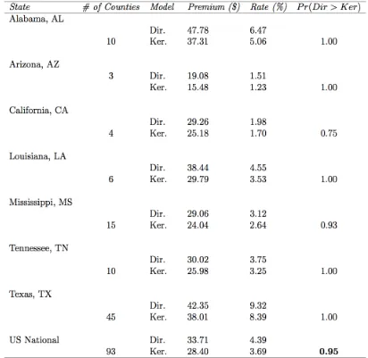
coverage level of 80%, 85%, and 90% respectively. The actuarial exercise is meant to examine the practical implications of our proposed Bayesian model compared to the nonparametric Kernel model. In all tables: we report state and national level aggregates (i.e., average) of estimated
Dir.) and Kernel (denoted by Ker.). State names are given in column 1. The second column shows the number of counties that are represented in a given state. We report the percentage of times (in
fraction) that both the premium and premium rates are larger in the Dirichlet Process Mixtures than the Kernel model in the last columns. Deriving the number of counties that both premium and premium rates are larger in the Dirichlet Process Mixtures than the Kernel model is therefore
straightforward. This can be achieved by multiplying the fraction by the corresponding number of available counties e.g., at the national level/entire cotton belt level: approximately 76 counties out
of the total of 93 had estimates from the Dirichlet model being larger. Similar logic can be applied to the state level estimates. The estimates for both insurance premium and premium rates are displayed in columns 1.4 and 1.5, respectively.
The results from Table 1.2, 1.3, 1.4 and 1.5 (i.e. 75%, 80%, 85%, and 90% coverage level) suggest the following. First, the proposed Dirichlet model yields actuarial estimates (e.g.,
premiums) that are larger than the Kernel counterpart both at the state and national levels. For example, the average premium over the entire cotton belt of the United States is $11.60/acre from the Dirichlet mixture model but $9.51/acre from the Kernel model from Table 1.2. Importantly,
this result hold strongly for the major cotton states such as Texas, Alabama, Mississippi and Tennessee. Second, the discrepancies of premiums between the Dirichlet model and Kernel model
notice that most counties that passed the selection criteria come from Texas as expected, and the number of counties from Texas correspond to about 48% of the total number of counties in the
cotton belt. In Texas, we find that 100% of the time, the Dirichlet model yield larger actuarial estimates than the Kernel.
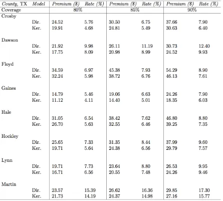
1.5.2. The Case of Texas and Visual Evidence
Empirical results using cotton yield data from only Texas are provided and discussed here. As emphasized earlier, Texas is a cotton hub and represents over 48% all eligible counties included
in the empirical analysis. Results for the case of Texas are presented using both visual and non-visual ways. Figures are used to report the estimated densities for selected counties in Texas, while the implied results from the insurance exercise are reported in tables. We restrict attention to eight
major counties from the Southern High Plains district, where our focus on these is motivated by the following. First, this district (and vis-à-vis the selected counties) is one of the leading cotton
producing belts in the United States; second, the district is characterized by low moisture and high elevation; and third, the district commonly experiences wide ranges and extremes in weather, particularly, temperature extremes.15 It is therefore useful and natural to observe that cotton yields
15 The whole notion of extreme weather or climate events may cover a broad facet of climate
densities in these higher risk production counties are complex; and our proposed Bayesian nonparametric model is able to effectively capture these complex yield densities. The eight
selected counties from Texas are displayed in Figure 1.4.
For comparison and consistency with the main results presented for the entire United States, we also display side-by-side results from both Bayesian nonparametric model, and the
nonparametric-Kernel model. As a baseline, we implement the rule-of-thumb criteria for choosing the bandwidth of a Gaussian kernel density estimator. Robustness checks for choosing different
bandwidth selection criteria such as Common Variation given by Scott (1992), using a Factor 1.06, Methods of Sheather and Jones (1991), unbiased and biased Cross-validation are also considered.
Figures 1.5-1.8 present pairs of estimated densities across the alternative models for eight
counties in Texas application: the Dirichlet processes mixture and a nonparametric-Kernel. The left panel in each figure corresponds to densities obtained from the Dirichlet processes mixture
while the right panels correspond to those from the Kernel-type approach. The figures demonstrate that the densities are visually comparable across the two approaches. The enormous flexibility of the Dirichlet model allows it to flexibly capture the probability distribution. In addition, there is
evidence that the left tail probabilities from the Dirichlet model are marginally larger than the Kernel. We will compare the left tails or estimated loss probabilities across the two models to
examine if they are quantitatively different from each other.
Table 1.6 reports the actuarial estimates for the eight selected counties in Texas and a robust nonparametric test of equality of the distribution of tail or loss probabilities obtained across the
two models.16 Before discussing the results, we briefly review the nonparametric test of distributional equivalence that we used (due Li 1996 and Li et al. 2009). Formally, denote the loss probabilities obtained from the Dirichlet and nonparametric Kernel by X and Z, respectively. The
testing framework uses an integrated square difference distance criterion
𝐼 = ℎ] 𝑥 − ℎH 𝑧 H𝑑𝑥𝑑𝑧
= ℎ] 𝑥 𝑑𝐻] 𝑥 + ℎH 𝑧 𝑑𝐻H 𝑧 − ℎ] 𝑥 𝑑𝐻H 𝑧 − ℎH 𝑧 𝑑𝐻] 𝑥
(1.13)
where the unknown probability density functions are estimated using kernel-based methods. Here
𝐻] . and 𝐻H . are the cumulative distribution functions for X and Z. The test statistic is derived
by replacing the first occurrences of objects ℎ] . and ℎH . by their leave-one-out kernel
estimates, and replacing 𝐻] . and 𝐻H . by their empirical distribution functions. A more
detailed presentation is available in (Li 1996, Li et al. 2009 and Hayfield and Racine 2008). One
advantage of the above statistical test which does not require the usual assumption of independence
16 Application to Entire Cotton Belt: The nonparametric test was also applied to test for equality
across the samples, which is an important departure from traditional approaches (e.g. Kolmogorov-Smirnov test and Cramér-von Mises test). Both the test statistic and corresponding probability
values (p-values) are reported in the last column of Table 1.6. We reject the null of distributional equivalence in all the counties at conventional levels of significance as the p-values are less than 0.01. In addition, the right panels of Figures 1.9 and 1.10 display the empirical cumulative
distribution functions of these loss probabilities for each of the eight major cotton counties in Texas. These figures also suggest visually that Dirichlet yield larger tail probabilities. Taken together, the
evidence suggest that the Dirichlet processes mixture produce tail or insurance loss probabilities that are quantitatively different from that of the nonparametric Kernel.
Consistent with results from the entire United States, the Texas results also indicate that
the Dirichlet model yield premium rates that are comparable but slightly higher than the Kernel (see Table 1.6 and Table 1.7). That holds for every coverage levels, 75%-90%. In fact, the rates
are even higher at a 90% coverage level which is consistent with the main results from the entire United States.
1.6. Conclusion
This paper proposes a Bayesian nonparametric model which is based on Dirichlet processes for yield estimation. We deploy our proposed model for the empirical estimation of county level yield data for Cotton from the entire United States. The implications of our modeling framework for the
model. First, the paper demonstrates using a conceptual proof that our proposed Dirichlet probability model outperforms the Kernel counterpart in simulated counterfactual worlds. Second,
the empirical analysis using the cotton belts data from the entire Unite States which involves the Group level insurance valuation documents the following: overall, our main results indicate that the proposed Dirichlet model provides slightly higher insurance premium rates than the Kernel
model, which can translate into large actuarial losses. Third, we carry over our analysis to only the case of Texas which is the major and leading cotton production state. With focus on eight major
cotton counties, we illustrate the following: we find that the Dirichlet model provide larger lower tail probabilities compared to the nonparametric Kernel. This in turn lead to slightly higher insurance premium rates under the Dirichlet model. The results are robust to alternative insurance
coverage levels and various Kernel bandwidth selection schemes.
Our interpretation is that the choice of density estimation approach could have important
implications for the pricing of insurance. The Bayesian nonparametric approach provides a promising alternative for the effective modeling and rating of insurance products. This can be especially important in regions where the underlying yield distributions are substantially complex.
The Bayesian nonparametric approach has not been given much attention in the insurance literature. The findings from this paper will largely simulate further research into much understanding and
Figure 1.1Counties in Cotton Belt for the United States
0 1
Note: Navy-colored cells correspond to included counties. To be included, the county must have at least 46 years of continuous upland-cotton yield history, United States.
(a) QQ Distribution Plots for 49 iterations
(b) QQ Distribution Plots for 99 iterations
.06 .08 .1 .12 .14 .16 Tru e-p re mi um ra te s
.07 .08 .09 .1 .11 DPM-rates
Q-Q Plot: Prem. Rates
.06 .08 .1 .12 .14 .16 Tru e-p re mi um ra te s
.06 .07 .08 .09 KNL-rates
Q-Q Plot: Prem. Rates
Number of iterations: 49
.06 .08 .1 .12 .14 .16 T ru e -p re mi u m ra te s
.07 .08 .09 .1 .11
DPM-rates Q-Q Plot: Prem. Rates
.06 .08 .1 .12 .14 .16 T ru e -p re mi u m ra te s
.06 .07 .08 .09 .1
KNL-rates Q-Q Plot: Prem. Rates
(c) QQ Distribution Plots for 499 iterations
Figure 1.3 QQ Distribution Plots
.06 .08 .1 .12 .14 .16 T ru e -p re mi u m ra te s
.06 .08 .1 .12
DPM-rates
Q-Q Plot: Prem. Rates
.06 .08 .1 .12 .14 .16 T ru e -p re mi u m ra te s
.04 .06 .08 .1 .12
KNL-rates
Q-Q Plot: Prem. Rates
Figure 1.4 Counties in Texas for Cotton Production
Note: The Eight−8 counties included are displayed in bold.
(a) Density Distributions by Using DPM and Kernel for Crosby
(b) Density Distributions by Using DPM and Kernel for Dawson
Figure 1.5 Densities: Crosby and Dawson ●●●●●●●●●●●●●●●●●●●●●●●●●●●●●●●●●●●●●●●●●●●●●●●●●●●●●●●●●●●●●●●●●●●●●●●●●●●●●●●●●●●●●●●●●●●●●●●●●●●●●●●●●●●●●●●●●●●●●●●●●●●●●●●●●●●●●●●●●●●●●●●●●●●●●●●●●●●●●●●●●●●●●●●●●●●●●●●●●●●●●●●●●●●●●●●●●●●●●●●●●●●●●●●●●●●●●●●●●●●●●●●●●●●●●●●●●●●●●●●●●●●●●●●●●●●●●●●●●●●●●●●●●●●●●●●●●●●●●●●●●●●●●●●●●●●●●●●●●●●●●●●●●●●●●●●●●●●●●●●●●●●●●●●●●●●●●●●●●●●●●●●●●●●●●●●●●●●●●●●●●●●●●●●●●●●●●●●●●●●●●●●●●●●●●●●●●●●●●●●●●●●●●●●●●●●●●●●●●●●●●●●●●●●●●●●●●●●●●●●●●●●●●●●●●●●●●●●●●●●●●●●●●●●●●●●●●●●●●●●●●●●●●●●●●●●●●●●●●●●●●●●●●●●●●●●●●●●●●●●●●●●●●●●●●●●●●●●●●●●●●●●●●●●●●●●●●●●●●●●●●●●●●●●●●●●●●●●●●●●●●●●●●●●●●●●●●●●●●●●●●●●●●●●●●●●●●●●●●●●●●●●●●●●●●●●●●●●●●●●●●●●●●●●●●●●●●●●●●●●●●●●●●●●●●●●●●●●●●●●●●●●●●●●●●●●●●●●●●●●●●●●●●●●●●●●●●●●●●●●●●●●●●●●●●●●●●●●●●●●●●●●●●●●●●●●●●●●●●●●●●●●●●●●●●●●●●●●●●●●●●●●●●●●●●●●●●●●●●●●●●●●●●●●●●●●●●●●●●●●●●●●●●●●●●●●●●●●●●●●●●●●●●●●●●●●●●●●●●●●●●●●●●●●●●●●●●
0 200 400 600 800
0.0000
0.0005
0.0010
0.0015
0.0020
Crosby: Dirichtlet Process Mixture
Yields
Density
●
●●●●●●●●●●●●●●●●●●●●●●●●●●●●●●●●●●●●●●●●●●●●●●●●●●●●●●●●●●●●●●●●●●●●●●●●●●●●●●●●●●●●●●●●●●●●●●●●●●●●●●●●●●●●●●●●●●●●●●●●●●●●●●●●●●●●●●●●●●●●●●●●●●●●●●●●●●●●●●●●●●●●●●●●●●●●●●●●●●●●●●●●●●●●●●●●●●●●●●●●●●●●●●●●●●●●●●●●●●●●●●●●●●●●●●●●●●●●●●●●●●●●●●●●●●●●●●●●●●●●●●●●●●●●●●●●●●●●●●●●●●●●●●●●●●●●●●●●●●●●●●●●●●●●●●●●●●●●●●●●●●●●●●●●●●●●●●●●●●●●●●●●●●●●●●●●●●●●●●●●●●●●●●●●●●●●●●●●●●●●●●●●●●●●●●●●●●●●●●●●●●●●●●●●●●●●●●●●●●●●●●●●●●●●●●●●●●●●●●●●●●●●●●●●●●●●●●●●●●●●●●●●●●●●●●●●●●●●●●●●●●●●●●●●●●●●●●●●●●●●●●●●●●●●●●●●●●●●●●●●●●●●●●●●●●●●●●●●●●●●●●●●●●●●●●●●●●●●●●●●●●●●●●●●●●●●●●●●●●●●●●●●●●●●●●●●●●●●●●●●●●●●●●●●●●●●●●●●●●●●●●●●●●●●●●●●●●●●●●●●●●●●●●●●●●●●●●●●●●●●●●●●●●●●●●●●●●●●●●●●●●●●●●●●●●●●●●●●●●●●●●●●●●●●●●●●●●●●●●●●●●●●●●●●●●●●●●●●●●●●●●●●●●●●●●●●●●●●●●●●●●●●●●●●●●●●●●●●●●●●●●●●●●●●●●●●●●●●●●●●●●●●●●●●●●●●●●●●●●●●●●●●●●●●●●●●●●●●●●●●●●●●●●●●●●●●●●●●●●●●●●●●●●●●●●●●
0 200 400 600 800
0.0000
0.0005
0.0010
0.0015
0.0020
Crosby: Nonparametric Kernel
Yields Density ● ● ●●●●●●●●●●●●●●●●●●●●●●●●●●●●●●●●●●●●●●●●●●●●●●● ● ●●●●●● ● ●●● ●●● ● ● ●●●● ● ●●● ● ● ●●● ● ● ●●●●●●●●●●●●●●●●●●●●●●●●●●●●●●●●●●●●●●●●●●●●●●●●●●●●●●●●●●●●●●●●●●●●●●●●●●●●●●●●●●●●●●●●●●●●●●●●●●●●●●●●●●●●●●●●●●●●●●●●●●●●●●●●●●●●●●●●●●●●●●●●●●●●●●●●●●●●●●●●●●●●●●●●●●●●●●●●●●●●●●●●●●●●●●●●●●●●●●●●●●●●●●●●●●●●●●●●●●●●●●●●●●●●●●●●●●●●●●●●●●●●●●●●●●●●●●●●●●●●●●●●●●●●●●●●●●●●●●●●●●●●●●●●●●●●●●●●●●●●●●●●●●●●●●●●●●●●●●●●●●●●●●●●●●●●●●●●●●●●●●●●●●●●●●●●●●●●●●●●●●●●●●●●●●●●●●●●●●●●●●●●●●●●●●●●●●●●●●●●●●●●●●●●●●●●●●●●●●●●●●●●●●●●●●●●●●●●●●●●●●●●●●●●●●●●
0 100 200 300 400 500
0.0000 0.0005 0.0010 0.0015 0.0020 0.0025 0.0030
Dawson: Dirichtlet Process Mixture
Yields Density ●●●●●●●●●●●●●●●●●●●●●●●●●●●●●●●●●●●●●●●●●●●●●●●●●●●●●●●●●●●●●●●●●●●●●●●●●●●●●●●●●●●●●●●●●●●●●●● ● ●●●●●●● ●●●●●● ● ●●●● ●●●●●●●●●●●●●●●●●●●●●●●●●●●●●●●●●●●●●●●●●●●●●●●●●●●●●●●●●●●●●●●●●●●●●●●●●●●●●●●●●●●●●●●●●●●●●●●●●●●●●●●●●●●●●●●●●●●●●●●●●●●●●●●●●●●●●●●●●●●●●●●●●●●●●●●●●●●●●●●●●●●●●●●●●●●●●●●●●●●●●●●●●●●●●●●●●●●●●●●●●●●●●●●●●●●●●●●●●●●●●●●●●●●●●●●●●●●●●●●●●●●●●●●●●●●●●●●●●●●●●●●●●●●●●●●●●●●●●●●●●●●●●●●●●●●●●●●●●●●●●●●●●●●●●●●●●●●●●●●●●●●●●●●●●●●●●●●●●●●●●●●●●●●●●●●●●●●●●●●●●●●●●●●●●●●●●●●●●●●●●●●●●●●●●●●●●●●●●●●●●●●●●●●●●●●●●●●●●●
0 100 200 300 400 500
0.0000 0.0005 0.0010 0.0015 0.0020 0.0025
Dawson: Nonparametric Kernel
Yields
(a) Density Distributions by Using DPM and Kernel for Floyd
(b) Density Distributions by Using DPM and Kernel for Gaines
Figure 1.6 Densities: Floyd and Gaines
● ● ● ●
●●●●●●●●●●●●●●●●●●●●●●●●●●●●●●●●●●●●●●●●●●●●●●●●●●●●●●●●●●●●●●●●●●●●●●●●●●●●●●●●●●●●●●●●●●●●●●●●●●●●●●●●●●●●●●●●●●●●●●●●●●●●●●●●●●●●●●●●●●●●●●●●●●●●●●●●●●●●●●●●●●●●●●●●●●●●●●●●●●●●●●●●●●●●●●●●●●●●●●●●●●●●●●●●●●●●●●●●●●●●●●●●●●●●●●●●●●●●●●●●●●●●●●●●●●●●●●●●●●●●●●●●●●●●●●●●●●●●●●●●●●●●●●●●●●●●●●●●●●●●●●●●●●●●●●●●●●●●●●●●●●●●●●●●●●●●●●●●●●●●●●●●●●●●●●●●●●●●●●●●●●●●●●●●●●●●●●●●●●●●●●●●●●●●●●●●●●●●●●●●●●●●●●●●●●●●●●●●●●●●●●●●●●●●●●●●●●●●●●●●●●●●●●●●●●●●●●●●●●●●●●●●●●●●●●●●●●●●●●●●●●●●●●●●●●●●●●●●●●●●●●●●●●●●●●●●●●●●●●●●●●●●●●●●●●●●●●●●●●●●●●●●●●●●●●●●●●●●●●●●●●●●●●●●●●●●●●●●●●●●●●●●●●●●●●●●●●●●●●●●●●●●●●●●●●●●●●●●●●●●●●●●●●●●●●●●●●●●●●●●●●●●●●●●●●●●●●●●●●●●●●●●●●●●●●●●●●●●●●●●●●●●●●●●●●●●●●●●●●●●●●●●●●●●●●●●●●●●●●●●●●●●●●●●●●●●●●●●●●●●●●●●●●●●●●●●●●●●●●●●●●●●●●●●●●●●●●●●●●●●●●●●●●●●●●●●●●●●●●●●●●●●●●●●●●●●●●●●●●●●●●●●●●●●●●●●●●●●●●●●●●●●●●●●●●●●●●●●●●●●●●●●●●●●●●●●●●●●●●●●●●●●●●●●●●●●●●●●●●●●●●●●●●●●●●●●●●●●●●●●●●●●●●●●●●●●●●●●●●●●●●●●●●●●●●●●●●●●●●●●●●●●●●●●●●●●●●●●●●●●●●●●●●●●●●●●●●●●●●●●●●●●●●●●●●●●●●●●●●●●●●●●●●●●●●●●●●●●●●●●●●●●●●●●●●●●●●●●●●●●●●●●●●●●●●●●●●●●●
0 200 400 600 800 1000
0.0000
0.0005
0.0010
0.0015
Floyd: Dirichtlet Process Mixture
Yields Density ● ● ● ● ●●●●●●●●●●●●●●●●●●●●●●●●●●●●●●●●●●●●●●●●●●●●●●●●●●●●●●●●●●●●●●●●●●●●●●●●●●●●●●●●●●●●●●●●●●●●●●●●●●●●●●●●●●●●●●●●●●●●●●●●●●●●●●●●●●●●●●●●●●●●●●●●●●●●●●●●●●●●●●●●●●●●●●●●●●●●●●●●●●●●●●●●●●●●●●●●●●●●●●●●●●●●●●●●●●●●●●●●●●●●●●●●●●●●●●●●●●●●●●●●●●●●●●●●●●●●●●●●●●●●●●●●●●●●●●●●●●●●●●●●●●●●●●●●●●●●●●●●●●●●●●●●●●●●●●●●●●●●●●●●●●●●●●●●●●●●●●●●●●●●●●●●●●●●●●●●●●●●●●●●●●●●●●●●●●●●●●●●●●●●●●●●●●●●●●●●●●●●●●●●●●●●●●●●●●●●●●●●●●●●●●●●●●●●●●●●●●●●●●●●●●●●●●●●●●●●●●●●●●●●●●●●●●●●●●●●●●●●●●●●●●●●●●●●●●●●●●●●●●●●●●●●●●●●●●●●●●●●●●●●●●●●●●●●●●●●●●●●●●●●●●●●●●●●●●●●●●●●●●●●●●●●●●●●●●●●●●●●●●●●●●●●●●●●●●●●●●●●●●●●●●●●●●●●●●●●●●●●●●●●●●●●●●●●●●●●●●●●●●●●●●●●●●●●●●●●●●●●●●●●●●●●●●●●●●●●●●●●●●●●●●●●●●●●●●●●●●●●●●●●●●●●●●●●●●●●●●●●●●●●●●●●●●●●●●●●●●●●●●●●●●●●●●●●●●●●●●●●●●●●●●●●●●●●●●●●●●●●●●●●●●●●●●●●●●●●●●●●●●●●●●●●●●●●●●●●●●●●●●●●●●●●●●●●●●●●●●●●●●●●●●●●●●●●●●●●●●●●●●●●●●●●●●●●●●●●●●●●●●●●●●●●●●●●●●●●●●●●●●●●●●●●●●●●●●●●●●●●●●●●●●●●●●●●●●●●●●●●●●●●●●●●●●●●●●●●●●●●●●●●●●●●●●●●●●●●●●●●●●●●●●●●●●●●●●●●●●●●●●●●●●●●●●●●●●●●●●●●●●●●●●●●●●●●●●●●●●●●●●●●●●●●●●●●●●●●●●●●●●●●●●●●●●●●●●●●●●●●●
0 200 400 600 800 1000
0.0000
0.0005
0.0010
0.0015
Floyd: Nonparametric Kernel
Yields
Density
●●●●●●●●●●●●●●●●●●●●●●●●●●●●●●●●●●●●●●●●●●●●●●●●●●●●●●●●●●●●●●●●●●●●●●●●●●●●●●●●●●●●●●●●●●●●●●●●●●●●●●●●●●●●●●●●●●●●●●●●●●●●●●●●●●●●●●●●●●●●●●●●●●●●●●●●●●●●●●●●●●●●●●●●●●●●●●●●●●●●●●●●●●●●●●●●●●●●●●●●●●●●●●●●●●●●●●●●●●●●●●●●●●●●●●●●●●●●●●●●●●●●●●●●●●●●●●●●●●●●●●●●●●●●●●●●●●●●●●●●●●●●●●●●●●●●●●●●●●●●●●●●●●●●●●●●●●●●●●●●●●●●●●●●●●●●●●●●●●●●●●●●●●●●●●●●●●●●●●●●●●●●●●●●●●●●●●●●●●●●●●●●●●●●●●●●●●●●●●●●●●●●●●●●●●●●●●●●●●●●●●●●●●●●●●●●●●●●●●●●●●●●●●●●●●●●●●●●●●●●●●●●●●●●●●●●●●●●●●●●●●●●●●●●●●●●●●●●●●●●●●●●●●●●●●●●●●●●●●●●●●●●●●●●●●●●●●●●●●●●●●●●●●●●●●●●●●●●●●●●●●●●●●●●●●●●●●●●●
0 100 200 300 400 500 600
0.000
0.001
0.002
0.003
0.004
Gaines: Dirichtlet Process Mixture
Yields
Density
●●●●●●●●●●●●●●●●●●●●●●●●●●●●●●●●●●●●●●●●●●●●●●●●●●●●●●●●●●●●●●●●●●●●●●●●●●●●●●●●●●●●●●●●●●●●●●●●●●●●●●●●●●●●●●●●●●●●●●●●●●●●●●●●●●●●●●●●●●●●●●●●●●●●●●●●●●●●●●●●●●●●●●●●●●●●●●●●●●●●●●●●●●●●●●●●●●●●●●●●●●●●●●●●●●●●●●●●●●●●●●●●●●●●●●●●●●●●●●●●●●●●●●●●●●●●●●●●●●●●●●●●●●●●●●●●●●●●●●●●●●●●●●●●●●●●●●●●●●●●●●●●●●●●●●●●●●●●●●●●●●●●●●●●●●●●●●●●●●●●●●●●●●●●●●●●●●●●●●●●●●●●●●●●●●●●●●●●●●●●●●●●●●●●●●●●●●●●●●●●●●●●●●●●●●●●●●●●●●●●●●●●●●●●●●●●●●●●●●●●●●●●●●●●●●●●●●●●●●●●●●●●●●●●●●●●●●●●●●●●●●●●●●●●●●●●●●●●●●●●●●●●●●●●●●●●●●●●●●●●●●●●●●●●●●●●●●●●●●●●●●●●●●●●●●●●●●●●●●●●●●●●●●●●●●●●●●●●●
0 100 200 300 400 500 600
0.000
0.001
0.002
0.003
Gaines: Nonparametric Kernel
Yields