The R6 Defect Assessment Procedure: Status and Key Recent Developments

THE R6 DEFECT ASSESSMENT PROCEDURE:

STATUS AND KEY RECENT DEVELOPMENTS

Peter J Budden1 and John K Sharples2

1

R6 Lead Engineer, EDF Energy, UK

2

Structural Integrity Consultant, Amec Foster Wheeler, Clean Energy, UK

ABSTRACT

The R6 procedure for the assessment of the integrity of structures containing defects has been continuously developed since 1976 to meet the needs of the UK power industry for defect tolerance arguments supporting the continued operation of nuclear power plant. It is routinely used by EDF Energy for the fracture assessment of metallic components in its Advanced Gas-Cooled Reactor (AGR) and Pressurised Water Reactor (PWR) fleet. As the plant ages, requirements to minimise unnecessary conservatism increase, and the challenges to maintaining margins increase. Hence the potential for the use of novel, more advanced methods also grows.

This paper first summarises the current status of the R6 documentation and its maintenance and development programme. Particular developments in three technical areas are then briefly highlighted: (1) the treatment of welding residual stress in fracture assessments, including bounding residual stress profiles and numerical simulation of residual stress; (2) the treatment of secondary stresses in fracture assessment, including the interaction of primary and secondary stress; and (3) limit load solutions. Other ongoing key developments are also briefly outlined.

INTRODUCTION

The R6 procedure (EDF Energy, 2015) was first published in 1976. Fracture mechanics was being used in the design assessment of proposed new civil nuclear plant in the UK; in particular, R6 was used for the pre-service safety case for the Sizewell PWR. At the time of its first issue, a failure assessment diagram (FAD) was used to assess elastic-plastic fracture and plastic collapse by evaluating the ratio, Sr, of

primary load to limit load based on flow stress, σf, defined as the average of the 0.2% proof stress, σy, and

the ultimate tensile stress, σu. The shape of the failure assessment curve, f(Sr), and hence the value of the

J-integral crack driving force, was defined by a strip-yielding approximation, with fracture conceded when Kr =f(Sr) where, for primary loads alone, Kr is the ratio of stress intensity factor to fracture

toughness. The scope of R6 was expanded by the issue of Revisions 1 and 2 in 1977 and 1980, respectively. However, the first major update was Revision 3 in 1986. This introduced the current notation Lr for the abscissa on the FAD, where Lr is defined using σy for the limit load, so that

r y f r ( / )S

L = σ σ . Collapse is conceded at L L f / y 1

max r

r = =σ σ > . Options were also introduced for the

shape of the failure assessment curve, Kr =f(Lr), with Option 2 a material-specific curve based on the

reference stress J-estimation scheme (Ainsworth, 1984), and Option 1 an explicit function of Lr derived as

an approximate lower bound to Option 2 curves for a range of austenitic and ferritic steels.

alternative, more advanced procedures, Chapter IV stress analysis and residual stress profile inputs, and Chapter V comprising validation and worked examples. Since 2001, a series of Amendments have been issued, the most recent being in March 2015 as Amendment 11.

Maintenance and development of R6 is managed by EDF Energy under a Structural Integrity Assessment Procedures collaboration which involves Amec Foster Wheeler, Rolls-Royce, TWI, Frazer-Nash Consultancy and NRG, Netherlands. R6 continues to be developed by EDF Energy and its partners to meet the requirements for the defect tolerance leg of safety cases, primarily driven by the requirements of the UK AGR and PWR nuclear reactors, the challenges of ageing plant, and the research requirements of the UK civil nuclear industry regulator, the Office for Nuclear Regulation (ONR).

This paper first briefly summarises the principal content of the changes to R6 Revision 4 at Amendment 11 and then provides some more detail of recent work in three particular technical areas: welding residual stress; secondary stress; and limit loads. However, the R6 programme covers work in a number of other technical areas, the details depending on priorities and varying over time. These currently include leak rate calculation methods (e.g. Gill, 2014) probabilistic leak-before-break arguments (e.g. Bhimanadam and Blom, 2014), FAD methods for notch-like defects (e.g. Horn and Budden, 2014), load history effects such as warm pre-stress (e.g. Teng and Sharples, 2012), and constraint effects due to thin sections (e.g. Kulka and Sherry, 2012) or residual stresses.

CHANGES TO R6 AT AMENDMENT 11

Amendment 11 has introduced revisions to 19 sections within Chapters I-IV of R6 and added one new section in Chapter V. The major changes are to: Section II.6 on the treatment of secondary stresses; Sections II.4 and IV.1 on limit loads; and to Sections II.7, III.15 and IV.4, including a new Section V.6, on welding residual stresses. These developments are summarised in the following three sections of this paper. Additionally, the leak-before-break methodology of Section III.11 has been updated to refer to recent work under the R6 programme on evaluating the crack opening area under both elastic-plastic and creep conditions (e.g. Madew et al., 2011), and to offer additional advice on determination of an appropriate local or global surface roughness, dependent on the crack opening, for use in determining friction factors and hence leak rates (e.g. Taggart and Budden, 2008). These are not described further in this paper. Minor changes have been made to Section II.1 on tensile properties and Section II.2 on fracture toughness values to maintain these sections up-to-date. The other revisions to R6 at Amendment 11, including to the status notes of Section I.12, are principally to reflect the significant changes to the methodology of Section II.6, in particular the use of the multiplicative V factor alone to quantify the effect of the interaction between primary and secondary stresses on the R6 Kr parameter, and hence the

corresponding estimate of J, with the earlier additive ρ term being removed.

WELDING RESIDUAL STRESSES

R6 Section II.7 gives advice on the treatment of weld residual stress and describes methods for estimating the corresponding stress distribution. It refers in particular to the residual stress compendium of R6 Section IV.4, and to R6 Section III.15 on numerical simulation of weld residual stress for austenitic materials that was issued in 2009. In addition, validation and worked example sheets for the calculation of residual stress in weldments have been incorporated in R6 Sections V.5 and V.6, respectively. At Amendment 11, additional advice has been added to Section II.7 on evaluating the stress intensity factor due to residual stress, on validation of the post-weld heat treatment rules from BS7910:2013 and on a range of residual stress measurement methods. On stress intensity factor, KI evaluation, it has been noted

that KI can be calculated using solutions for arbitrary applied stress distributions when these are available

components may be more readily available. Methods for determining the self balancing component are suggested in the text and also in the status notes.

The residual stress compendium of Section IV.4 contains upper bound residual stress profiles (so-called Level 2 profiles) for a range of common welded joints including: Plate Butt and Pipe Seam Welds, Pipe Butt Welds, T-Butt Welds, Nozzles, Repair Welds, Transition Welds and Weld T-Intersections. Annual reviews of new information are undertaken to maintain R6 Section IV.4 up-to-date, but have not led to major revisions to Section IV.4 in recent years. However, for Amendment 11, slight modifications have been made such that the recommended profiles are now fully consistent with the recent advice in BS7910:2013 (British Standards, 2013), and additional advice has been added to cover both ferritic and austenitic steels for the range of weldment geometries addressed.

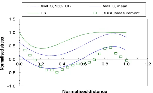
Development of statistical methods, Teng and Bate (2014), Mathew et. al. (2014) has been ongoing to improve the current Level 2 profiles. A heuristic method has been developed for determining residual stress profiles, Teng et al. (2008), based on a combination of the weighted least-squares method and the application of expert judgement. This has been applied to the residual stress data used to determine the current profiles for transverse stresses in pipe girth welds and to more recent measurement data. The method was used to generate a mean residual stress profile based on the combination of the membrane, bending and self-balancing components. An upper bound profile was then determined on the basis of 95% confidence limits. An example is shown in Figure 1, where stress and distance through the pipe wall are normalised by the 0.2% proof stress and wall thickness, respectively. This compares the mean residual stress profile determined using the heuristic method (AMEC, mean) with measured Block Removal Splitting and Layering (BRSL) data for a low carbon micro-alloyed steel pipe, X52, submerged arc (SAW) girth weld from He et al. (2010). Also shown is the R6 Level 2 profile for low heat input welds. The figure shows that the upper bound profile determined using the heuristic approach (AMEC, 95% UB) is not as conservative as the current Level 2 profile but still provides a reasonable upper bound to the measured data. A neural network approach has also been developed to characterise through-thickness residual stress profiles in austenitic steel girth welds, Mathew et al. (2014). The network was trained using measured data collated by Bouchard (2007). An upper bound profile determined using the neural network approach has been compared to the neutron diffraction measurements on experiments from the European STYLE project, Keim et al. (2014). Based on the work described above and other complementary studies, including the provision of additional experimental data, the recommended transverse and longitudinal residual stress profiles for pipe girth welds are planned to be revised based on an analysis of the enhanced database using the developed statistical methods. Furthermore, it is proposed to introduce new upper bound residual stress profiles for electron beam welds. These are likely to be based on studies undertaken by Hurrell et al. (2014) on four electron beam welded specimens: 316L plate, 304L pipe, SA508-3 forging and an A533B plate.

-1.0 -0.5 0.0 0.5 1.0 1.5

0.0 0.2 0.4 0.6 0.8 1.0 1.2

No

rm

a

li

s

e

d

s

tr

e

s

s

Normalised distance

AMEC, 95% UB AMEC, mean

R6 BRSL Measurement

Figure 1. Comparison of residual stress profiles with axial residual stress measurements on a low carbon micro-alloyed SAW pipe girth weld, He et. al. (2010)

Work is ongoing to extend the guidance for austenitics and for ferritic materials and dissimilar metal welds where phase changes need to be considered in the modelling process. The validation part of the guidelines provide “standards” against which the predicted stresses can be validated. A series of “Weld Residual Stress Benchmarks” are being developed for inclusion in R6 Sections V.5 and V.6. These describe welded mock-ups in which residual stresses have been measured using various techniques. Users can refer to these when validating their finite element modelling techniques and thus provide greater confidence in the predicted results. A number of welded mock-ups have been generated to support a European collaborative round-robin and industrial research programmes, Bate et al. (2012), Bate (2013). These include an austenitic single bead-on-plate weldment, the information of which was introduced in Section V.5 of R6 in 2011, and an austenitic groove welded plate, the information of which has been introduced at Amendment 11 in Section V.6 (Figure 2). Planned validation cases include an austenitic pipe girth weld, an austenitic repair weld, a ferritic groove weld and a ferritic bead-on-plate weldment.

Figure 2. Validation example – austenitic groove weld

SECONDARY STRESSES

The R6 approach to quantifying the contribution of secondary stresses to fracture is to modify the definition of the Kr parameter, leaving Lr unchanged so that secondary stresses by definition in R6 do not

following equation, with the superscripts p and s on the stress intensity factor KI or J-integral denoting

primary and secondary, respectively:

mat s I p I

r (K VK )/K

K = + , equivalent to J=(Kp_I +VKs_I)2/(E′(f(L_r)2) (1)

with E′=E/(1−ν2), where E and ν are Young’s modulus and Poisson’s ratio, respectively. The V and ρ approaches are based on the same underlying J-estimation methodology so the results of an assessment are essentially independent of the choice of method. All recent developments in the R6 approach to treating secondary stresses have been based on V so at Amendment 11 it was decided to remove ρ and to focus on the use of V. It should be noted that the use of a multiplicative factor on the secondary terms is consistent with that employed in both the API 579-1/ASME FFS-1 (2007) and RSE-M (AFCEN, 2005) procedures.

At Amendment 11, R6 Section II.6 has been re-written. The “simplified V procedure” has been retained but with a lower limiting value of V of 0.4 at high values of Lr rather than the previous lower limit on V

of unity. This corresponds to an allowance for mechanical stress relief of the secondary stress, noting that V < 1 is equivalent to ρ < 0. The previous “detailed V procedure” has been retained without change with

ξ

=(K /K )

V s_J s_I where KsJ = E′Js and values of ξ are tabulated as a function of Lr and r pI s J s

J =K L /K

β .

The main changes to Section II.6 are in the provision of a range of additional options to the user.

Firstly, a second “detailed procedure” is set down where (Ainsworth, 2012) ξ is expressed as an explicit function of Lr alone:

(

)

r r r

r s I s

J/K )f(L ) 0.42L (0.72 L ){f(L )}

K (

V= + + (2)

with f(Lr) being the shape of the failure assessment curve that is used in the overall failure assessment. A

comparison of the tabular and Equation (2) approaches to ξ is shown in Figure 3.

0 0.2 0.4 0.6 0.8 1 1.2 1.4

0 0.5 Lr 1 1.5 2

Table - Table - Equation (2)

1

s J= β

4

s J= β

ξ

Figure 3. Comparison of the detailed approaches for ξ based on tabulated values and Equation (2)

Secondly, new guidance on elastic follow-up is introduced into Section II.6. The approaches to estimating

ξ allow VKs_I /Ks_J =ξ>1at small values of Lr, up to a maximum of about 1.2 using Equation (2). At larger

values, VKs_I/Ks_Jfalls below unity corresponding to plastic relaxation of secondary stress. The estimates are intended to be conservative relative to typical behaviour. However, it is known that in some cases

s J s I /K

VK can be less than unity for all values of Lr and, in other cases, the maximum value of s

J s I /K

assessor. The cases where VKs_I /Ks_J is significantly greater than unity correspond to significant elastic follow-up where the basic procedures, which are appropriate to low or moderate follow-up, are not appropriate. In cases of significant follow-up, two alternatives are now given. The first is to treat the secondary stress as primary in the calculation of V; this leads to (Ainsworth, 2012):

) L ( f ) L ( f L ) L ( f ) L ( ) ( f K K V _s r s s r r r r s s s I s J β + β β + − + β β = (3)

where βs=Ks_IL_r /Kp_I. The second option involves the use of an elastic follow-up factor, Z. Such a factor has been used for some time for creep crack growth under combined loading in the R5 procedure (EDF Energy, 2014) but its explicit use is new to R6. Section II.6 refers to R5 for the quantification of Z. For Z<3, the simplified and detailed R6 approaches are adequate. However, for Z>3, an estimate of V is

      + β − + = s J s I 2 r r s r r s I s J K K )} L ( f ){ L ( L Z 1 Z 75 . 0 ) L ( f K K V (4)

Secondary stress acting as primary corresponds to the limit Z→∞. However, Equation (4) does not fully capture the approach of Equation (3) in this limit, but does reduce to it for small values of primary and secondary loads with L_r +β≤0.7and so sensitivity studies should be performed when large values of Z are obtained.

For cases of multiaxial remote stresses with significant stress parallel to the defect plane, an estimate of V for cases of moderate elastic follow-up is given, following James (2010), as

2 / 1 mod ref mod ref 2 y mod ref mod ref mod ref r s I s J ) / E ( ) / ( A E ) L ( f K K V −         σ ε σ σ − σ ε = (5)

where A=0.8σ₁p/σ_Misesp and Lr y/1.25

mod ref = σ

σ with εmod_ref denoting the strain on the material uniaxial

stress-strain curve at the modified reference stress, σmod_ref . The factor of 0.8 in the expression for A was chosen for conservatism based on a range of finite element calculations and applies for uniform remote tensile stress. For remote bending, σp_I and σ_Misesp are the peak bending stress divided by 3 and 3/2,

respectively. More generally, σ_Misesp can be defined from the limit load for the uncracked section with

ref p

Mises=σ

σ and σp_I as the peak tensile stress. This approach may be used for sensitivity studies, particularly when there are remote applied stresses parallel to the defect plane, but is not applicable to cases of large elastic follow-up.

previous methods in Section II.6. It was shown that there are significant load-order effects for large secondary stresses but these are successfully treated by the new methods in R6 Section II.6.

LIMIT LOADS

The limit load is one of the principal inputs to R6; it defines the parameter Lr and hence quantifies

proximity to plastic collapse, and to fracture via the definition of the failure assessment curve Kr = f(Lr).

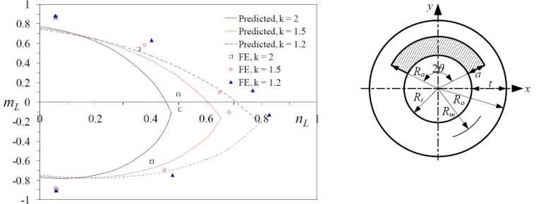
Equivalently, for primary loads alone, it leads to an estimate of the J-integral as Jp =K2/E′f2(L_r). A compendium of limit loads for defective homogeneous test specimens, plates, cylinders and spheres, under various loads, was included in R6 Revision 4 as Section IV.1 and has been updated several times since 2001. At Amendment 11, the previous solutions in R6 Section IV.1 for circumferential defects in thin-walled cylinders under combined internal pressure, p, axial tension, N, and global bending, M, have been extended to general thick-walled solutions by Lei et al (2014a). Some comparisons of the solutions against detailed finite element limit load calculations have also been reported by Li et al. (2014). An example is shown in Figure 4, where nL and mL are normalised limit values of N and M. Generally, the

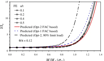
analytical limit loads are conservatively lower than the finite element data. The solutions have also been used with R6 Option 2 to compare the estimated J-values with published data for a range of cylinder radius to thickness ratios, crack sizes, loading types and material strain hardening exponents, n; see Figure 5 for an example. The J-data have also been used to give better advice in R6 Section II.4 for both axial and circumferential defects in cylinders. In particular, cases where the global limit loads are conservative for J-estimation are more clearly identified and, in other cases, the previous advice that factors of 0.8 to 0.9 on the global limit load are sometimes necessary to ensure conservatism is confirmed; e.g. Figure 5 (Lei, 2013).

The treatment of defects in pipe bends has been extended in R6 Section II.4 to include references to sources of information on stress distributions in the uncracked bend under various pressure and bending situations, which can be used to construct approximate limit loads for the defective bends.

Recent work via the R6 programme has concentrated on extending the scope of the recommended limit loads to more complex geometries, such as pipe bends and pipe branches, and to more complex loading conditions, for example plates under biaxial loading conditions. Although, published limit load solutions for both cracked and uncracked pipe bends have been reviewed within EDF Energy, explicit advice for inclusion in R6 Section IV.1 awaits further finite element J-solutions, and also the development of corresponding stress intensity factor solutions for R6 Section IV.3.

Figure 5. External semi-elliptical surface crack, cylinder under bending, θ π= 0.12, k =1.25, n=10 (Lei, 2013). J is normalised by the corresponding elastic value, Je and M by its limit value, ML

The case of the limit load for an extended surface crack in a plate under combined biaxial force and through-thickness bending is separately addressed in this conference by Aird and Lei (2015) who compare finite element values of the limit load with theoretical estimates of Lei and Budden (2014). The latter are shown to be conservative in general, that is, lower than the corresponding finite element values. Some numerical validation of the R6 solution, by means of comparison of R6 Option 2 J-estimates with published J values, was given by Lei et al. (2014b). The theoretical solutions have recently been generalised to surface defects of finite length by Lei and Budden (2015). These solutions for biaxial loading will be included in future updates to R6 following suitable validation against estimates of J. The stress intensity factor is not affected by the force parallel to the crack front so changes to R6 Section IV.3 will not be required.

CONCLUSIONS

This paper has briefly described the evolution and current status of the R6 procedure. Recent developments in the areas of welding residual stresses, secondary stresses and limit loads have been described. The paper has also discussed ongoing work in the R6 programme, focussing on these 3 technical areas, which is expected to lead to further enhancements to R6 advice in the future. The changes to R6 Revision 4 at Amendment 11 have been highlighted and include the following.

●The advice on numerical simulation of welding residual stress in austenitic steels in R6 Section III.15 has been improved by the use of mixed isotropic-kinematic hardening models.

●The upper bound, Level 2 welding residual stress profiles in R6 Section IV.4 are now fully consistent with the recent advice in BS7910:2013, and additional advice has been added to cover both ferritic and austenitic steels for the range of weldment geometries addressed.

● Additional advice has been added to R6 Section II.7 on evaluating the stress intensity factor due to residual stress, on validation of the post-weld heat treatment rules from BS7910 and on the range of residual stress measurement methods.

●A new R6 Section V.6 has been added as a worked example of the Section III.15 approach.

● The treatment of secondary stress in R6 Section II.6 now uses the multiplicative V factor alone. The conservatism of the simplified V route has been lessened for values of Lr greater than unity by allowing

for mechanical stress relief of the secondary loading.

● A range of new detailed approaches for treating secondary stresses has been added which include methods based on quantifying elastic follow-up and multiaxiality of the remote loads. Improved advice is given on situations where follow-up may be significant.

● The previous global limit load solution for thin-walled circumferentially-cracked cylinders under combined tension, global bending and internal pressure in R6 Section IV.1 has been extended to

thick-0 5 10 15

0.0 0.2 0.4 0.6 0.8 1.0 1.2 1.4

M/ML(σ0)

J/

Je

0.1 0.2 0.4 0.5

Predicted (Opt-2 FAC based) Predicted (Opt-1 FAC based) Predicted (Opt-2, 80% limit load) FE a/t

walled cylinders. The advice on the use of global limit loads for cylinders with axial or circumferential cracks in R6 assessments has been expanded and clarified.

ACKNOWLEDGEMENTS

This paper was produced as part of the R6 development programme and is published by permission of EDF Energy and Amec Foster Wheeler. The authors acknowledge the contributions of colleagues in the R6 programme to the work summarised herein and R Ainsworth for his comments on this paper.

REFERENCES

AFCEN (2005). “RSE-M: In-service inspection rules for mechanical components of PWR nuclear islands”, 1997 Edition plus 1998, 2000 and 2005 Addenda, Paris.

Ainsworth, R. A. (1984). “The assessment of defects in strain hardening material”, Engng Frac. Mech., 19, 633-642.

Ainsworth, R. A. (1986). “The treatment of thermal and residual stresses in fracture assessments”, Engng

Frac. Mech., 24, 65-76.

Ainsworth, R. A., Sharples, J. K. and Smith, S. D. (2000). “Effects of residual stresses on fracture behaviour – experimental results and assessment methods”, J Strain Analysis, 35, 307-316. Ainsworth, R. A., Bannister, A. C. and Zerbst, U. (2001). “An overview of the European flaw assessment

procedure SINTAP and its validation”, Int. J. Pres. Ves. Piping, 77, 869-876.

Ainsworth, R. A. (2012). “Consideration of elastic follow-up in the treatment of combined primary and secondary stresses in fracture assessments”, Engng Frac. Mech., 96, 558-569.

Aird, C. J. and Lei, Y. (2015). “Comparison of analytical and finite element based limit loads for wide plates containing an extended surface crack under combined biaxial forces and cross-thickness bending”, Trans. SMiRT-23, August, Manchester.

American Petroleum Institute/ASME (2007). “Fitness-for-Service”, API 579-1/ASME FFS-1, Washington DC.

Bate, S., Shallcross, N., Stone, K., Francis, J., Mark, A. and Gill, C. (2012), “Development of material model parameters suitable for the finite element simulation of ferritic welds”, Paper PVP2012-78299, Proc. ASME PVP Conference, July, Toronto.

Bate, S. (2013). “The development of ferritic weld benchmarks for validating residual stress weld simulations”, Trans. SMiRT-22, August, San Francisco.

Bhimanadam, V. R. and Blom, F. J. (2014). “Probabilistic fracture analysis of circumferentially cracked pipes”, Paper PVP2014-28150, Proc. ASME PVP Conference, 20-24 July, Anaheim.

Bouchard, J. (2007). “Validated residual stress profiles for fracture assessments of stainless steel pipe girth welds”, Int. J. Pres. Ves. Piping, 84,195-222.

British Standards Institution (2013). “Guide to methods for assessing the acceptability of flaws in metallic structures”, BS7910:2013, London.

EDF Energy (2015). “R6: Assessment of the integrity of structures containing defects”, Revision 4, with amendments to Amendment 11, Gloucester.

EDF Energy (2014). “R5: Assessment procedure for the high temperature response of structures”, including revisions to Revision 002, Gloucester.

Gill, P. J. (2014). “A coupled fluid-solid model to investigate leak rates for leak-before-break sssessments”, Paper PVP2014-28170, Proc. ASME PVP Conference, 20-24 July, Anaheim. He, W., Wei, L. and Smith, S. (2010), “Intensive validation of computer prediction of welding residual

stresses in a multi-pass butt weld”, 29th Int. Conf. on Offshore Mech. and Arctic Engng (OMAE),

June, China.

Hurrell, P. R., Pellereau, B. M. E., Gill, C. M., Kingston, E., Smith, D. and Bouchard, P. J. (2014), “Development of residual stress profiles for defect tolerance assessments of thick section electron beam welds”, Paper PVP2014-28809, Proc. ASME PVP Conference, 20-24 July, Anaheim. James, P. (2010). “Treatment of secondary and residual stresses: guidance to R6 regarding the interaction

of primary and secondary stresses from work performed between 2005-09”, Serco Report SERCO/TAS/3375.03/001 Issue 2, Warrington.

James, P. (2015a). “Calculation of KJ under secondary loads in isolation for R6”, Proc ASME PVP

Conference, Paper PVP215-45274, July 19-23, Boston.

James, P. (2015b). “Investigation into load order effects on the treatment of combined primary and secondary stresses within R6”, Trans. SMiRT-23, Manchester.

Keim, E., Sharples, J. and Nicak, T. (2014), “FP7 project STYLE: Implications and recommendations, discussion”, Proc. ASME PVP Conference, Paper PVP2014-28254, July, Anaheim.

Kulka, R. S. and Sherry, A. H. (2012), “Fracture toughness evaluation in C(T) specimens with reduced out-of-plane constraint”, Proc. ASME PVP Conference, Paper PVP2012-78751, July, Toronto. Lei, Y. (2013). “Numerical validation of limit load solutions for defective cylinders in R6”, EDF Energy

Report E/REP/BBGB/0114/GEN/13, Gloucester.

Lei, Y. and Budden, P. J. (2014). “Limit load solutions of plates with extended cracks under combined biaxial forces and cross-thickness bending”, J. Strain AnalysisAnalysis

,

Lei, Y., Li, Y. and Gao, Z. (2014a). “Global limit load solutions for thick-walled cylinders with circumferential cracks under combined internal pressure, axial force and bending moment – part I: theoretical solutions”, Int. J. Pres. Ves. Piping, 114-115, 23-40.

Lei, Y., Budden, P. J. and Aird, C. J. (2014b). “The effect of biaxial loading on the limit load and J estimates for plates with extended surface cracks, 20th European Conference on Fracture, Trondheim, Procedia Materials Science, 3, 667-672.

Lei, Y. and Budden, P. J. (2015). “Global limit load solutions for plates with surface cracks under combined biaxial forces and cross-thickness bending”, under review.

Li, Y., Lei, Y. and Gao, Z. (2014). “Global limit load solutions for thick-walled cylinders with circumferential cracks under combined internal pressure, axial force and bending moment – part II: finite element validation”, Int. J. Pres. Ves. Piping, 41-60, 23-40.

Madew, C., Sharples, J., Charles, R. Gill, P. and Budden, P. (2011), “The evaluation of crack opening areas for through-wall cracks in the vicinity of pipe branch connections”, Proc. ASME PVP

Conference, Paper PVP2011-57312, July 17-21, Baltimore.

Mathew. J, Moat, R. J. and Bouchard, P. J. (2014), “Optimised neural network prediction of residual stress profiles for structural integrity assessment of pipe girth welds”, Proc. ASME PVP

Conference, Paper PVP2014-28845, July, Anaheim.

Oh, C.-Y., Nam, H.-S., Kim, Y.-J., Ainsworth, R. A. and Budden, P. J. (2014). “FE validation of R6 elastic-plastic J estimation for circumferentially cracked pipes under mechanical and thermal loadings”, Engng Fract. Mech., 124-125, 64-79.

Song, T.-K., Oh, C.-Y., Kim, Y.-J., Ainsworth, R. A. and Nikbin, K. (2013). “Approximate J estimates for combined primary and secondary stresses with large elastic follow-up”, Int. J. Pres. Ves.

Piping, 111-112, 217-231.

Taggart, J. P. and Budden, P. J. (2008). “Leak before break: studies in support of new R6 guidance on leak rate evaluation”, J. Pres. Ves. Tech., 130(1), 011402.

Teng. H., Bate. S. K. and Beardsmore. D. W. (2008), “Statistical analysis of residual stress profiles using a heuristic method”, Proc. ASME PVP Conference, Paper PVP2008-61378, July, Prague.

Teng, H. and Bate, S. (2014). “Residual stress profiles of pipe girth weld using a stress decomposition method”, Proc. ASME PVP Conference, Paper PVP2014-28247, July, Anaheim.

Teng, H. and Sharples, J. K. (2012). “Further predictions of fracture experiments of a pre-cracked pressurised thermal shock disk specimen under warm prestressing loading cycles”, Proc. ASME