ABSTRACT
CHEW, KRISTEN RAE. The Use of Osteometric Sorting Techniques to Aid in the
Resolution of a Large Scale Commingling: The Piggot Ossuary Site (31CR14). (Under the direction of Dr. Ann H. Ross, Dr. Chelsey Juarez, and Dr. D. Troy Case).
The purpose of this study was to utilize gross and osteometric sorting techniques as a
first approach in the sorting of commingled human remains. The Piggot ossuary site
(31CR14), curated at the Forensic Analysis Laboratory at North Carolina State University
was used because it as a large-scale commingling of human remains. The minimum number
of individuals (MNI) was estimated at 53. The MNI was calculated using the right humerus,
which was the skeletal element and side most represented in the assemblage.
The sample used in this study consists of 114 skeletal elements. Each individual element was
assigned an identification number. All bones were measured according to standard and
non-standard measurements and recorded in a Microsoft Excel spreadsheet.In cases of
fragmentation, only available measurements were taken. All t-distributions were performed
in Excel; regression equations were derived in SPSS Statistics 19.0.0, and Student’s t-tests were calculated using GraphPad Software.
Visual pair matching, the association of left and right elements based on parallels in
morphology, was conducted on all complete or nearly complete elements.Several elements
were successfully pair-matched and later confirmed with osteometric sorting.
The basic principle of osteometric sorting is that the two bones being considered are
of a similar size and shape to have originated from the same individual. Osteometric sorting
depends on the ability to distinguish anatomically normal size and shape relationships among
standard deviations. The JPAC-CIL database was utilized because it contained both standard
and non-standard measurements that are specific to fragmented remains.
Three models were used in the osteometric sorting process. Model one compares left
and right sides, which accounts for shape differences, similar to visual pair-matching and in
many cases performs equally as well. Model two compares joint surfaces of bone elements
based on the size of articulating surfaces. Model three compares bones of different sizes. The
null hypothesis for all three models is that the bones are of a similar size and to some extent,
shape to have originated in a single individual. A p-value of <0.10 indicates that the two bones being considered are significantly different and does not support the null hypothesis.
Results show that the use of osteometric sorting is a good first approach. In the case
of the Piggot ossuary site (31CR14), elements were sorted into groups of similar shape and
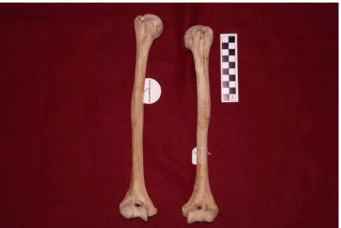
size, rather than into individuals. In one case, it was possible to pair two humeri. This was
© Copyright 2014 Kristen Chew
The Use of Osteometric Sorting Techniques to Aid in the Resolution of a Large Scale Commingling: The Piggot Ossuary Site (31CR14)
by Kristen Chew
A thesis submitted to the Graduate Faculty of North Carolina State University
in partial fulfillment of the requirements for the degree of
Master of Arts
Anthropology
Raleigh, North Carolina
2014
APPROVED BY:
_______________________________ ______________________________
Dr. Ann Ross Dr. D. Troy Case
Committee Chair
DEDICATION
This thesis is dedicated to my Nan. She has been my best friend and my mentor throughout
my entire life. I miss her every day and continue to push myself to be the best that I can, for
her. I would also like to dedicate this thesis to my very best friend Quinn. She has been my
driving force when times get tough. She is there when I am absolutely sure that I cannot
BIOGRAPHY
Kristen Rae Chew wrote the entirety of this Master’s thesis at Cup A Joe in Raleigh,
North Carolina. She went to the University of Central Florida in Orlando, Florida for her
Bachelor of Arts where she fell in love with forensic anthropology and bioarchaeology. She
attended graduate school at North Carolina State University where she earned her Master of
Arts in Anthropology.
Her hobbies outside of school include running, reading, and astronomy. She is
currently training for her first half marathon, which she will complete in February 2015 with
her best friend. Her favorite astronomical body is the Orion Nebula, which she spent many
nights contemplating through her telescope when graduate school got tough.
She plans to pursue a PhD in anthropology and eventually a career as a professor in
ACKNOWLEDGMENTS
First and foremost, I want to thank my graduate advisor, Dr. Ann H. Ross for her
mentorship and friendship throughout the past two years and in the years to come. She taught
me the necessary skills that will lead me into my future with confidence; she believed in me
when I struggled and encouraged me when I doubted my abilities. She patiently answered my
questions and allowed me to learn from my mistakes, all the while waiting on the sidelines,
not letting me stray too far from the right path. I realized that knowledge can be learned from
a book and taught by most anyone, but the life skills, personal lessons, and confidence that I
need to go along with it can only be taught by a very unique person with a very special gift
for giving, a gift of patience, and a gift of understanding. That person is Dr. Ross, who is my
mentor and now my friend and again I thank her. I would also like to thank Dr. Chelsey
Juarez for her invaluable advice and her constant lessons on professionalism and the
development of my career. It took time and much patience from her, but she never showed
frustration. McKay said it best; “True education does not consist merely in the acquiring of a
few facts of science, history, literature, or art, but in the development of character.” These
lessons will last into the future and once again, I am truly grateful. I would also like to thank
Dr. D. Troy Case for his help with the thesis editing process and his invaluable help adjusting
to graduate school and talking through issues. Finally, I would like to thank Dr. John E. Byrd
for his help as a technical consultant on my thesis and for the opportunity to visit the JPAC
labs and work with the folks on the “K-208” project where I learned the methods to complete
TABLE OF CONTENTS
LIST OF TABLES ... vii
LIST OF FIGURES ... ix
CHAPTER 1: Introduction ...1
CHAPTER 2: Review of the Literature ...4
Early Skeletal Sorting Techniques ...5
Transitional Sorting Techniques ...9
Osteometric Sorting Techniques ...12
CHAPTER 3: Historical Background ...17
Ossuary Burials ...17
The Late Woodland Period (800-1650CE) ...21
Summary and Conclusion ...25
CHAPTER 4: Materials and Methods ...26
Materials ...26
The Piggot Ossuary...26
JPAC-CIL Database ...28
Methods ...29
Data Collection ...30
Minimum Number of Individuals ...31
Osteometric Sorting ...31
CHAPTER 5: Results ...35
Model One Results ...35
Model Two Results ...38
Model Three Results ...41
Student’s t-test ...45
Juvenile Results ...45
Overall Findings ...50
CHAPTER 6: Discussion ...51
CHAPTER 7: Conclusion ...59
Limitations ...59
REFERENCES ...61
APPENDICES ...65
APPENDIX I: Measurement Definitions ...67
APPENDIX II:D-values for Models One and Two ...74
Model One ...74
Model Two ...75
APPENDIX III: T-values for Models One, Two, and Three...77
Model One ...77
Model Two ...79
LIST OF TABLES
Table 2.1 Table of Articulations ...7
Table 4.1 Radiocarbon date as reported for the Piggot Site (31CR14) ...28
Table 5.1 Results for Model 1: Clavicle ...37
Table 5.2 Results for Model 1: Humerus ...37
Table 5.3 Results for Model 1: Radius ...37
Table 5.4 Results for Model 1: Ulna ...37
Table 5.5 Results for Model 1: Os Coxa ...38
Table 5.6 Results for Model 1: Femur ...38
Table 5.7 Results for Model 1: Tibia ...38
Table 5.8 Results for Model 2: Left Femoral Head and Acetabulum ...40
Table 5.9 Results for Model 2: Right Femoral Head and Acetabulum ...40
Table 5.10 Results for Model 2: Left Femur and Left Tibia ...40
Table 5.11 Results for Model 2: Right Femur and Right Tibia ...40
Table 5.12 Regression Results for Model 3 ...41
Table 5.13 Results for Model 3: Humerus to Clavicle ...43
Table 5.14 Results for Model 3: Humerus to Radius ...43
Table 5.15 Results for Model 3: Humerus to Ulna ...43
Table 5.16 Results for Model 3: Humerus to Femur ...43
Table 5.17 Results for Model 3: Femur to Tibia ...44
Table 5.18 Results for Model 3: Femur to Fibula ...44
Table 5.19 Student’s t-Test Results for Comparison of Left and Right Sides ...45
Table 5.20 Results for Juvenile Clavicle ...47
Table 5.21 Results for Juvenile Scapula ...47
Table 5.22 Results for Juvenile Humerus ...47
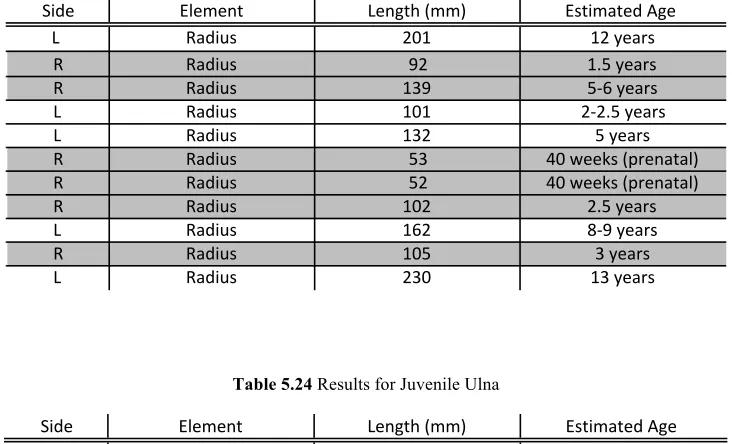
Table 5.23 Results for Juvenile Radius ...48
Table 5.24 Results for Juvenile Ulna ...48
Table 5.25 Results for Juvenile Ilium ...48
Table 5.26 Results for Juvenile Femur ...49
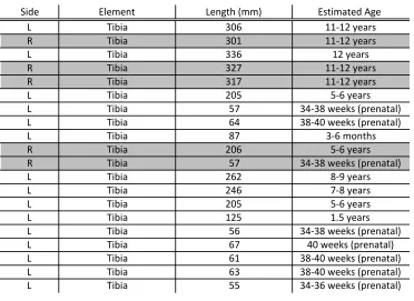
Table 5.27 Results for Juvenile Tibia ...50
Table 6.1Range of Variation for Femur ...56
Table 8.1 Measurement Definitions ...67
Table 8.2 D-values for the Clavicle ...74
Table 8.3 D-values for the Humerus ...74
Table 8.4 D-values for the Femur ...74
Table 8.5 D-values for the Os Coxa ...75
Table 8.6 D-values for the Radius ...75
Table 8.7 D-values for the Ulna ...75
Table 8.8 D-values for the Tibia ...75
Table 8.10 D-values for the Right Femur to the Acetabulum ...76
Table 8.11 D-values for the Left Femur to the Left Tibia ...76
Table 8.12 D-values for the Right Femur to the Right Tibia ...76
Table 8.13 T-values for the Clavicle ...77
Table 8.14 T-values for the Humerus ...77
Table 8.15 T-values for the Femur ...77
Table 8.16 T-values for the Os Coxa ...78
Table 8.17 T-values for the Radius ...78
Table 8.18 T-values for the Tibia ...78
Table 8.19 T-values for the Ulna ...79
Table 8.20 T-values for the Left Femur to the Acetabulum ...79
Table 8.21 T-values for the Right Femur to the Acetabulum ...79
Table 8.22 T-values for the Left Femur to the Left Tibia ...80
Table 8.23 T-values for the Right Femur to the Right Tibia ...80
Table 8.24 T-values for the Humerus to the Clavicle ...80
Table 8.25 T-values for the Humerus to the Radius ...80
Table 8.26 T-values for the Humerus to the Ulna ...81
Table 8.27 T-values for the Humerus to the Femur ...81
Table 8.28 T-values for the Femur to the Tibia ...81
LIST OF FIGURES
Figure 3.1 Feast of the Dead ...20
Figure 3.2Protohistoric Ethnic and Linguistic Groups in NC Coastal Plain ...23
Figure 4.1 Radiocarbon Date as Reported for the Piggot Site (31CR14) ...27
Figure 6.1 Model 1: Left and Right Humerus ...52
Figure 6.2 Model 1: Two Right Humeri ...53
Figure 6.3 Results of Data Cleaning Process from Adams and Byrd (2002) ...55
Chapter 1: Introduction
Commingling refers to the situation where more than one individual is represented in
an assemblage, and have become mixed together (Ubelaker 2002). The sorting of individuals
in a commingled assemblage is imperative in the realms of forensic anthropology and
bioarchaeology. The segregation of remains into individuals is important in several aspects of
study. These range from the biological profile to the study of health of a population to
positive identification of victims. Numerous methods are currently employed for the
segregation of commingled human remains. These include aging (e.g. epiphyseal union),
matching articular surface morphology, visual pair matching, osteometric sorting, the use of
taphonomy, and DNA analysis (Byrd 2008).
Initial efforts to sort commingled human remains includes the development of
methods that estimate the number of individuals present and sort those individuals based on
similarities in bone morphology (Snow and Folk 1970). Developments in other fields such as
zooarchaeology, initiated quantitative methods to estimate the minimum number of
individuals (MNI) (Adams and Konigsberg 2004). As the methods were further developed,
the sorting of commingled remains began to rely more heavily on the use of statistics and
more advanced equations were developed using osteometrics and bone measurements (Byrd
and Adams 2003; Byrd 2008).
There are strong correlations among the sizes of bones. If someone has a large
humerus, you can expect that they will have a large femur. Osteometric sorting virtually
Adams 2003). Osteometric sorting uses size measures of the unmatched elements and
compares these to the same skeletal elements in a reference sample. Segregation decisions
are made by testing the null hypothesis that the two specimens of interest are of a similar
enough size and shape to have originated from a single individual (Byrd 2008). Osteometric
sorting takes advantage of the fact that the human physique will vary in predictable ways
(Byrd and Adams 2003). In addition, the relatively simple statistics, low error rates and
inexpensive nature make osteometric sorting an ideal method for the reassociation of skeletal
elements in a commingled context (Byrd and Adams 2003; Byrd 2008).
In this study, the Piggot ossuary (31CR14) is used because it is a large-scale
commingling of an archaeological context. Ossuaries are secondary deposits of skeletal
remains from multiple individuals. Excavation and study of ossuaries require assessment of
commingling (Ubelaker 2002). The complexity of a commingled assemblage is dependent on
the overall number of dead involved and the preservation of the remains. Therefore,
commingling can be broadly categorized into two types: small-scale and large-scale (Byrd
and Adams 2003; Mundorff et al 2008). The degree of commingling and/or fragmentation
determines the scale demarcation. For example, a large sample size with a low level of
comingling would be considered a small-scale commingling. Also considered a small-scale
commingling, a small number of individuals represented but extensive mixing of skeletal
elements. A large-scale commingling involves large numbers of individuals whose bodies are
mixed in a random manner or involve a large amount of fragmentation (Mundorff et al 2008).
Assemblages that are primarily fragmentary can present difficulties. Since standard
(Buikstra and Ubelaker 1994), these measurements cannot be used on fragmentary remains.
Byrd and Adams (2003) created measurements that are designed for areas of the bone that
typically survive the taphonomic processes, which allows for measurements to be taken
without the complete bone being present. Even with the development of these measurements,
there are cases where association cannot be made without the aid of DNA analysis.
The main focus of this study is to use osteometric sorting along with other
morphological techniques such as taphonomy and visual pair-matching to aid in the
resolution of the large-scale commingling of the Piggot ossuary site (31CR14). The goal is
not to test the efficacy of osteometric sorting. Standard measurements (Buikstra and
CHAPTER 2: Review of the Literature
Commingling is problematic in a variety of forensic and bioarchaeological settings.
Regardless of whether the analysis is of an ossuary or a mass disaster, the commingling of
human remains complicates the process from recovery to final disposition. In cases where
victims are known, such as an aircraft crash, it is still an arduous task to sort the remains.
However, in this instance a positive identification is likely. A flight manifest can be
consulted and victims’ family members can be contacted to provide DNA samples. When the
victims are unknown, sorting of the remains, and positive identification becomes much more
difficult due to the uncertainty of the individuals involved. In both cases, multiple techniques
must be utilized to sort the remains into individuals.
To date, there has been a paucity of research addressing the issue of commingling.
Krogman’s (1986) work, The Human Skeleton in Forensic Medicine, does not mention commingling as a problem in the identification of remains. T. Dale Stewart’s (1979),
Essentials of Forensic Anthropology, dedicated only 2 of 300 pages to the issues surrounding
commingling in forensic settings. He claims that commingling is not usually an issue in
forensic anthropology because many of the materials recovered suggest the presence of a
single individual (Stewart 1979). However, commingling does present itself as an issue in
both forensic anthropology and bioarchaeology and skeletal biologists must apply their
scientific techniques to develop a resolution (Ubelaker 2002). As they become more involved
in human rights violations and post-conflict investigations, these methods become
Early Skeletal Sorting Techniques
The techniques used for the sorting of commingled human remains are mainly
morphological (Ubelaker 2002). Visual pair-matching refers to the association of left and
right elements based on similar morphology. Visual pair matching on different skeletal
elements (e.g. a humerus and a femur) is not recommended because it is subjective in nature.
Adams and Byrd (2006) suggested that visual pair-matching can be accurately performed by
experienced osteologists with humeri, femora, and tibiae if the preservation is sufficient;
other elements were not formally tested (Adams and Konigsberg 2004).
Taphonomic agents can best be described as either physical objects or natural
processes that help transition the human body after death from above ground, to the ground
layer (Ubelaker 1997). Taphonomy is the “study of the transition of organic remains from the
biosphere into the lithosphere” (Efremov 1940; Behrensmeyer 1984; Haglund and Sorg
1996; Ubelaker 1997). Taphonomic patterning refers to the analysis similarities and
differences in preservation. These patterns can be used in the process of skeletal
re-association. Remains lying in different locations within a grave can be exposed to various
soil types with distinct properties and moisture levels, which can be used to segregate
individuals exposed to different processes during primary interment that were commingled
later. However, taphonomic differences can also be observed on the remains of a single
individual due to disarticulation and/or a variable burial context, such as in an ossuary where
remains are disarticulated and not necessarily buried with their associated elements. These
caution, since the conditions that create the patterns can easily affect portions of adjacent
skeletons (Kerley 1972).
Articular surface matching is one of the most reliable methods for sorting (Buikstra et
al. 1984). Joint articulations can be used to assess whether a bone forms a congruent juncture
with another skeletal element and a large portion of a skeleton can be re-articulated via these
joint articulations. When using joint articulations to re-associate a skeleton it is common to
start with the pelvis or vertebrae. However, the strength of the association differs depending
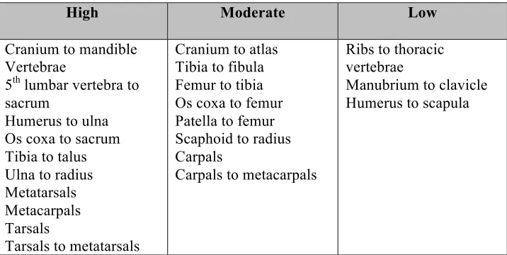
on the element in question (Adams and Byrd 2006). Table 2.1 outlines the strength of the
re-associations that Adams and Byrd (2006) assigned to different joints based on levels of
confidence, which were classified into high, moderate, and low. However, it should be noted
that these confidence levels were derived and assigned based solely on the authors’
experience and not developed from a controlled study. Problems with articulation result from
the absence of a close fit between particular elements. The articulation between the head of
the humerus and the glenoid fossa on the scapula is not very diagnostic and the scapula is
very difficult if not impossible to associate with the rest of the skeleton. Other elements, such
Table 2.1 Table of articulations indicating the amount of confidence placed in a fit (adapted from Adams and Byrd 2006)
Charles Snow (1948) created the first procedures for sorting commingled human
remains by combining the aforementioned techniques. Initially, he reconstructed fragmented
elements. Then, long bones were sorted according to size similarities, shape, and
morphology. He notes that bones characterized by any incomplete epiphyseal unions or
arthritis should be segregated first. Snow (1948) recommends beginning the association of
elements with the axial skeleton and moving outward to the appendicular skeleton. He
developed this process while working at the Central Identification Laboratory (CIL) in
Hawaii in 1947. He states that for this process to work correctly, all elements from every
individual involved must be present. Therefore, this technique is rarely used as a complete
skeleton is not always available. One central component of this technique is that the process
of elimination can be utilized once visual pair matching and articulation have been executed,
High Moderate Low
Cranium to mandible Vertebrae
5th lumbar vertebra to
sacrum
Humerus to ulna Os coxa to sacrum Tibia to talus Ulna to radius Metatarsals Metacarpals Tarsals
Tarsals to metatarsals
Cranium to atlas Tibia to fibula Femur to tibia Os coxa to femur Patella to femur Scaphoid to radius Carpals
Carpals to metacarpals
Ribs to thoracic vertebrae
though in a large scale commingling, the ability to sort is lessened due to the increased
number of similar elements.
In 1957, Baker and Newman conducted a study on the use of dry bone weights for the
determination of living weight as a way to identify deceased individuals. They found that the
correlation between individuals is very general and not significant enough to make skeletal
weight an efficient predictor for exact living weight. They reported correlations at 0.544 for
whites and 0.392 for blacks. However, when comparing bone weight within an individual,
the correlation is substantial. They claim that any correlation of greater than 0.8 indicates that
the actual weight of one bone will correspond closely with the predicted weight of a second
bone. Those correlations falling below 0.7 can be expected to produce greater discrepancies.
This study was an important first step in the application of statistical analyses to the sorting
of commingled human remains. The authors (1957) recognize the importance of segregating
the commingled remains into individuals and present an attempt to remove the subjective
criteria of morphology.
Ellis Kerley (1972) noted the importance of training and experience when attempting
to first detect, and then sort commingled remains in an assemblage. He cautioned
investigators on the use of taphonomy as a sorting technique because the environmental
factors can vary widely. For example, if a humerus and a scapula of a single individual are
exposed to different soils they will express differing taphonomical patterns. Kerley (1972)
also pointed out the importance of the use of analytical techniques and their potential for the
Transitional Sorting Techniques
Eyman (1965) conducted a study using short-wave ultra-violet light sources applied
to human phalanges, which were soaked in an ultra-violet fluorescing pigment. This method
tested the discrimination between individuals in the same archaeological site as well as
individuals between archaeological sites. What they found was that the overall coloration
after immersion in the fluorescent media allowed for the geographic discrimination of
individuals based on soil composition, but that discrimination between individuals from a
single site was more complicated. The patterns of fluorescence seem to reflect the overall
architectural arrangement of the bone minerals, which are unique to each individual. These
patterns are unique to each individual and are prominent enough to allow for discrimination
among individuals (Eyman 1965). Overall, this method allows for the discrimination of
individuals between sites based on soil composition differences and also the discrimination
of individuals within a single site based on patterns in bone architecture. One issue with this
type of study is the permanent discoloration of the elements.
Snow and Folk (1970) conducted a study on identifying commingling in an
assemblage that does not include any duplicated elements. Duplication of elements is a clear
indication of commingling. Without duplication, it is still possible to detect commingling and
differentiate individuals based on sex, ancestry, age, and size. However, if the suspected
commingling involves individuals that are very similar, the traditional methods may not
detect the commingling. In their study, they provide an algorithm that expresses the
probability that undetected commingling is present. While this method can be useful
example, it assumes complete disarticulation of the skeleton and that the likelihood of it
appearing among recovered remains is equal for each bone, ignoring differences in size and
shape, which could lead to differential survival of elements when exposed to differing
weather conditions (Snow and Folk 1970). Despite the assumptions not always being true,
this can be useful in scenarios where similar individuals are commingled and the total
skeletal parts total less than one individual are present.
In the spring of 1998, construction at a private residence uncovered a large number of
human bones (Cruse 2002). The remains were fragmented and commingled. They were
brought to the bioanthropology laboratory at the College of Mount Saint Joseph for analysis.
Despite fragmentation, the remains were determined to be those of a Native American
population. The techniques used to sort the remains were: estimation of minimum number of
individuals (MNI), age-at-death estimation, and sex estimation. They were not concerned
with the association of each element to another, but with the overall sorting methods for the
creation of a biological profile of a population (Cruse 2002). In this instance, the use of
osteometric sorting may have increased their knowledge of individuals within the population
and provided additional biological information.
In a study by Tuller et al (2008), spatial analysis was used to analyze spatial
relationships among disarticulated and commingled remains in a mass grave. The study
suggests that a disarticulated element will be geographically closest to the skeleton it is
associated with. They found that 88% of the actual matching elements were closer to the
skeleton they belonged to, rather than all other potential matches. While spatial analysis
associations in ranked order (Tuller et al 2008). This can be useful in cases where there has
been little to no disturbance of the burial pit. Once there has been disturbance, the probability
that the associated elements will remain in close proximity to one another will likely decrease
significantly. This method is valuable because it allows for the remains to be studied while in
situ.
In a 2011 study, Nikita and Lahr considered the implications of obtaining a reliable
estimate of the number of individuals in a commingled assemblage. There are two different
types of estimators used to establish the composition of a sample prior to commingling
(Nikita and Lahr 2011). These two estimators are: 1) the minimum number of individuals
(MNI), which estimates the number of individuals in the sample based on the element and
side with the largest representation, and 2) the minimum likely number of individuals
(MLNI), which estimates the initial population represented in the sample. The estimation of
initial number of individuals represented in an assemblage (MLNI) assumes that the loss of
elements is random (i.e. that left and right elements have an equal chance of being altered or
removed from the sample) (Nikita and Lahr 2011). Obtaining an accurate estimate of the
number of individuals is important in forensic analyses for identification, especially in cases
of mass disaster. It is also important in the bioarchaeological context because it can provide
valuable information concerning paleodemographic information and mortuary behaviors
Osteometric Sorting Techniques
One of the first reliable studies to use statistics to resolve the issue of commingling
was Buikstra and colleagues (1984), in which they utilized measurements of adjoining bone
portions to assess the possibility that two cervical vertebrae originated from a single
individual based on similar size and shape. Measurements were taken on cervical vertebrae
from skeletons of Black females from the ages of 16 to 25 in the Terry Collection at the
Smithsonian Institution. The method was created by subtracting the measurement of the more
inferior element from that of the more superior element. This new measurement denoted the
“congruence” between adjacent elements. Then, a t-test was utilized to compare the new variable to the reference sample (Terry sample) mean. This allowed for the removal of the
subjective judgment of articulation.
In a similar study using osteometric sorting, London and Curran (1986) focused on
the articulation of the femoral head to the acetabulum. The authors called attention to the
significance of the metric relationship of the femoral head and the acetabulum. Their sample
consisted of 100 individuals from the Physical Anthropology Laboratories of the Maxwell
Museum, University of New Mexico. Their analysis outlined the efficacy of the hip joint in
the segregation of commingled human remains. The femoral and acetabular measurements
are highly paralleled suggesting that these measurements can be used to segregate
commingled human remains. However, the authors did not provide the details as to how this
conclusion was derived. London and Hunt (1998) retested this method utilizing 129
individuals from the Terry Collection following the London and Curran (1986) protocol. The
arthritic lipping. As a result, they revised the measurements to exclude the arthritic lipping
and postmortem changes. They tested the revised measurements on 30 “unknown”
individuals from the Huntington Collection and found that commingled remains were easily
segregated by using the measurements of the femoral head and acetabulum, and by using a
combination of the visual and morphometric data.
Similar to the methods proposed by Snow (1948), osteometric comparison is a
method that uses statistical models to objectively compare the size and shape relationship
between elements (Adams and Byrd 2006; Byrd and Adams 2003; Buikstra et al. 1984; Byrd
and Adams 1999). This method removes subjective judgment and offers a statistical
foundation for sorting of commingled remains. This method can be utilized when other
methods, such as visual pair-matching and articulation are not possible. It is stressed by
Adams and Byrd (2006) that the strength of osteometric sorting is to distinguish inconsistent
relationships that can lead to the exclusion of elements.
Osteometric sorting tests the null hypothesis that the two bones being considered are
of a similar enough size and shape to have originated from a single individual (Byrd 2008).
Byrd (2008) discusses three osteometric sorting models. The first model compares left and
right elements centering on shape. The second model compares articulating bone surfaces
based on size. The third model uses regression equations to compare the size of two different
elements, such as a femur and a humerus (Byrd 2008). Osteometric sorting utilizes a
reference dataset of measurements collected from known individuals that represents both
sexes and various ancestral groups (e.g. CILHI, Forensic Data Bank, Smithsonian Institution
University of Tennessee Bass Collection) (Byrd and Adams 2003). Standard measurements
(Buikstra and Ubelaker 1994) and measurements created for fragmentary remains are utilized
(Byrd and Adams 2003). It is essential to consider that the results from the three models can
be beneficial in eliminating individuals and to support a possible association, but the method
cannot not be used to prove an association.
Ubelaker (2002) performed a study of the commingled remains from an ossuary in
southern Maryland. First, a skeletal inventory of bone and side, separated by developmental
age was conducted in order to assess the minimum number of individuals (MNI). This was
done because most of the bone assemblage was secondary, meaning that they were primarily
interred elsewhere and moved at a later date, and lacked the articulations needed to relate the
bones to individuals. Using this method, they were able to estimate that there were at least
188 individuals present in the ossuary. Ubelaker (2002) suggests that a more detailed study
could have been completed by attempting to match pairs of bones, or arranging the immature
bones by approximate age. This could have been taken one step further to side each immature
bone and group each set of elements by age and maximum length in order to segregate those
elements that were too different to have originated in a single individual.
In the spring of 2003, a large grain bag filled with human skeletal remains was found
by bush cutters in a forest in South Africa. Differential taphonomy suggested that the
individuals had not died at the same time, or that they had decomposed under differing
conditions. The remains were sent to the University of Pretoria for analysis by L’Abbe
(2005). She utilized Snow’s (1948) and Byrd and Adams’ (2003) procedures for the
of elimination, and taphonomy. By using these methods, they were able to sort 155 of the
elements into ten individuals. The remainder of the elements were unable to be associated
with individuals. Sorting the skeletal elements into distinct individuals was complicated by
the context in which the remains were discovered and the large quantity of missing elements.
L’Abbe (2005) suggested that utilizing osteometric sorting may have increased the number of
elements that could be segregated.
Adams and Byrd (2006) conducted a study that involved the commingled skeletal
remains of two individuals who died in a helicopter crash in 1969 during the Vietnam War.
The techniques used to segregate the individuals were visual pair-matching, joint articulation,
process of elimination, taphonomy, and osteometric sorting. The first individual was
identified largely by the upper body and associated artifacts; the second individual was
identified by a distal right tibia and right foot inside of a military issued boot. Bones were
sorted by element type, side and size. Then visual pair-matching, articulation, process of
elimination, osteometric sorting, and taphonomy were utilized. Because there were only two
individuals represented in this case, articulation and process of elimination were successful.
The mandible that was recovered in 1969 was nearly complete and could be associated with
individual 1 via dental records. Therefore, the partial mandible could be associated with
individual 2 by process of elimination (Adams and Byrd 2006). The authors (2006) were also
able to associate remains using an orange-red colored rust discoloration resulting from the
metal from the helicopter. Based on the staining, it was obvious that the much of the remains
had been articulated before they were discovered. In this instance, the location of perimortem
humerus was fractured in conjunction with the proximal ends of a left ulna and a left radius.
Because of the fragmentation, articulation was not useful, but trauma found on all three
elements indicated that the fractures occurred while the arm was still articulated (Adams and
Byrd 2006). In this study, the authors were also able to associate a left humerus to a right
femur from individual 2 by using the measurements of the humeral and femoral heads
(Adams and Byrd 2006). Without this technique, the authors would most likely not have been
able to make this particular association. The authors recommend that sorting procedures are
to be employed in tandem with one another, not as standalone techniques (Adams and Byrd
2006). In some instances, however, it may be difficult or impossible to accomplish
segregation with these techniques and in these cases, it may be necessary to have some type
CHAPTER 3: Historical Background
Ossuary Burials
Ossuaries are mass graves containing the collected, often disarticulated, skeletal
remains of multiple individuals (Curry 1999). As defined, ossuaries are secondary graves,
meaning that the remains were originally buried or stored at another location, disinterred,
collected, and reburied in one common mass grave. Classically, these burials include two or
more stages: the removal of flesh from bones, through tools or natural decomposition;
storage of these cleaned bones; and the final reburial of the bones into a common grave
(Garret 2012). As a burial practice, the custom occurred from the Southeastern United States
to the Great Lakes area from late in prehistory into the early historic period (Curry 1999).
Despite their frequent occurrence, ossuaries remains poorly understood. This is due,
in part, to the lack of proper study. This can be attributed to the 19th century, before the
advent of “scientific archaeology,” or even today where accidental discovery of these sites
often takes place during construction and results in the further commingling or fragmentation
of the remains. Even though ossuary burials are poorly understood, the most commonly
studied and documented types are found in North America. These represent periodic
reburials, which sometimes involved several villages and were often done in conjunction
with an extravagant ceremony. The meaning of ossuary burials differs by culture; these
meanings range from religious ideas to mere practicality (Garrett 2012).
Bioarchaeologists are able to gather an assortment of information from remains in
population, pathology and general levels of health (Bogdan and Weaver 1992;Ubelaker
1974; Garrett 2012). These studies are conducted by compiling data through osteological
analyses like the estimations of sex and age, and estimating minimum number of individuals
and minimum likely number of individuals. Mortality and/or fertility rates can be estimated
through the analysis of ages-at-death; health and morbidity profiles can be estimated through
pathological analyses (Ubelaker 1974). Grave goods can be studied to assess social
organization and provide glimpses into past lifeways.
Archaeological and ethnohistorical data suggest that the Native American ossuaries
“contain nearly a complete representation of all individuals who died in the contributing
populations during a culturally represented number of years” (Ubelaker 1974: 59). North
American ossuary burials usually follow a broad pattern: bodies are allowed to decompose
through mechanical defleshing, cremation, or natural decomposition; remains are
periodically gathered and cleaned and occasionally bundled; they are then placed in
communal pits (Garrett 2012).
North American ossuaries occupy three general regions. These regions include 1)
Canada and the Great Lakes area, 2) the Southeastern region of the United States, and 3) the
Mid-Atlantic area of the United States. The Huron, of the Great Lake area, are best known
archaeologically for ossuary burial practices (Curry 1999; Ubelaker 1974). As documented
among the Huron, the burial rite was named the “Feast of the Dead” and began by placing the
body of the deceased in a temporary burial region. The body was then placed on a scaffold or
buried (Figure 3.1). Then, every eight to ten years or so, a village or group of villages would
their temporary locations, cleaned of any remaining flesh, and reburied in a communal burial
pit; the pit was lined with animal skins and the deceased were provided with goods for their
afterlife (Curry 1999; Ubelaker 1974). The community would hold a great feast during the
ceremony. This ceremony was first witnessed by the Jesuit missionary Jean de Brebeuf in
1636 in a Huron village in Ontario, Canada. Several other explorers, such as Samuel de
Champlain and Father Gabriel Sagard, a lay bother of the Franciscans, confirm the
documents of Brebeuf (Ubelaker 1974).
The accounts of the explorers illustrate the importance of ossuary burial practices
among the Huron people and the significance they attached to the details of the ceremony. It
has been said that the “Feast of the Dead” ceremony was the most important event in their
belief system, and that it was the most solemn ceremony they held (Ubelaker 1974).
Eventually, the Huron custom of ossuary burial was replaced by the Christian mortuary
practices. Some Iroquois still placate their dead with semi-annual feasts that are suggestive of
Burial customs in the Southeastern region of the United States include ceremonies
analogous to those described for the Huron, but with regional differences (Ubelaker 1974).
The best accounts of burial practices for this region are the archaeological record, since
ethnographic documentation is scarce. Romans (1999) documented that the Choctaw
practiced “bone cleaning” of the deceased; though the bones were cleaned by specialists who
travelled through the Choctaw nation instead of by relatives, like in the Huron practices
(Ubelaker 1974). The removed flesh was buried and the bones painted, placed in a chest,
which were then placed in a “bone house.” The method of final disposition of the remains
varied, with some groups leaving the bones in the temples forever (Ubelaker 1974).
Mortuary customs in the Mid-Atlantic area of the United States are best known from
the documentation of Captain John Smith and Thomas Hariot, and the drawings of John
White. They were all particularly interested in the treatment of the dead. Although Native
American mortuary practices were observed by multiple explorers, the ethnographical
accounts of burial practices are less consistent and the best documentation for ossuaries is the
archaeological record (Garrett 2012; Ubelaker 1974).
Ossuary burials throughout Virginia, Maryland, and southern Delaware are typically
linked with Iroquoian and Algonkian speaking groups. They are associated with the Middle
Woodland (200-800CE), Late Woodland (800-1650CE), and early Historic (ca. 1650CE)
periods (Curry 1999; Garrett 2012; Ubelaker 1974). These were varied in their burial
practices; those that contain characteristics of the Mid-Atlantic region can include both
articulated and disarticulated skeletons. In some cases, bones are in bundles, and in others,
they are scattered throughout the ossuary pit; some pits contain artifacts and others do not;
and some pits have been documented to contain cremated bones (Curry 1999; Garrett 2012;
Ubelaker 1974).
The Late Woodland Period (800-1650CE)
The Late Woodland phase indicates the emergence of linguistic, cultural, and
physical differences among populations that characterize the different tribes observed at the
time of European contact. The populations were differentiated by regional cultural variations;
these included language, material culture, settlement patterns, mortuary practices, and diet
(Hutchinson 2002, Phelps 1983, Ward and Davis 1999). Shell-tempered pottery marks the
Late Woodland period, which emerges during this time along the coast of North Carolina
North Carolina demonstrates cultural boundaries that were evident between the North
and South coastal regions. However, unlike other periods there were considerable differences
within the North coastal region itself. The Northern coastal region is divided into inner and
outer coastal regions, which are designated as the Cashie and Colington phases (Phelps 1983;
Ward and Davis 1999). The North outer coastal region, designated as the Colington phase,
extended from North Carolina’s major sounds to the barrier islands. This area was occupied
by Algonkian linguistic groups (see Figure 3.2). The Colington phase is distinct in its burial
methods, known as ossuaries, as discussed above.
Archaeological information regarding the size of Colington phase villages and
settlement patterns is restricted, although data suggests the existence of sedentary villages
after 1000CE (Hutchinson 2002; Ward and Davis 1999: Garrett 2012). At the time of contact,
Carolina Algonkians were structured by multiple ranked societies or chiefdoms. It has been
estimated that Carolina Algonkian towns contained 12 to 18 longhouses and about 120 to 200
individuals per town (Ward and Davis 1999). Colington phase sites were generally located
along major streams, sounds, and estuaries that provided them with the resources needed for
various subsistence activities such as farming, hunting, fishing, and foraging (Phelps 1983;
Figure 3.2 Protohistoric Ethnic and Linguistic Groups in the NC Coastal Plain (Phelps 1983; Garrett 2012)
Ossuary burials were the primary form of burial in the Late Woodland period
(800-1650CE) in the Southeastern United States. The Carolina Algonkians utilized large communal
ossuaries. Very little is known about mortuary customs of these ossuaries because of
insufficient documentation and varying accounts in early ethnographic records. Descriptions
regarding the treatment of the deceased are varied in their narratives. The disparities indicate
either inaccurate reporting among early explorers, or they reflect a great deal of variability in
Algonkian mortuary practices (Garrett 2012; Ubelaker 1974). Much of the ossuaries’
contents have been lost to looters and the taphonomic processes resulting from soil erosion,
Archaeologists have recognized three patterns of ossuary interment within North
Carolina. These correspond to the three geographical and ethnolinguistic regions during the
Late Woodland Period (800-1650CE). These are: 1) the outer Northern coastal
Algonkian-speaking groups; 2) the inner Northern coastal Iroquoian-Algonkian-speaking groups; and 3) the
Southern coastal Siouan-speaking groups (Loftfield 1990).
Algonkian ossuaries are usually large, communal burial sites, which contain the
disarticulated remains of a population spanning a period of time (Garrett 2012; Hutchinson
2002). The majority of Algonkian ossuaries contain between 20 and 60 individuals.
Skeletons are often commingled and are sometimes only represented by isolated bone
elements. Bundled remains are not common within these ossuaries. Grave goods are
comparatively rare when compared to Northern traditions. Additionally, Algonkian ossuaries
are differentiated from others within North Carolina by their placement along the coast,
relatively near the associated village (Garrett 2012; Hutchinson 2002; Loftfield 1990; Ward
and Davis 1999).
Iroquoian ossuaries, among the inner coastal region of North Carolina, tend to be
much smaller, containing the remains of family groups, usually only housing two to five
individuals. Bundling is common with distinct groupings in burial placement. Grave goods
are frequent, commonly including gravel-tempered ceramics and Marginella shell beads, totaling between 200 and 2000. These ossuaries are also frequently characterized by their
placement within villages, instead of on the margin (Garrett 2012; Hutchinson 2002;
Siouan ossuaries were comprised of small sand mounds, sometimes found on high
sand ridges, and contain the secondary remains of bundled individuals and sometimes
include charred remains. Artifacts are sometimes present within the mound with grave
offerings documented at some sites. These burial mounds are characteristically located away
from areas of habitation. This mortuary practice is common in southeastern North Carolina
and is possibly related to similar burial mounds in Georgia (Garrett 2012; Loftfield 1990).
Summary and Conclusions
Ossuaries have been documented in an assortment of contexts. Nevertheless, the
ossuaries found among Native North Americans fit within Ubelaker’s (1974) definition of
‘true’ ossuaries, which are secondary burial deposits representing the collective and periodic
reinterment of individuals after a culturally prescribed number of years. Although ossuary
burials are widespread throughout North America, moderately little research has been
dedicated to their analysis, which is likely due to various issues such as commingling,
CHAPTER 4: Materials and Methods
Materials
The Piggot Ossuary
The Piggot ossuary collection is comprised of skeletal remains from the Piggot site
(31CR14), which is located on the coast of North Carolina, inside Carteret County near
Gloucester. The ossuary was located on a ridge facing “The Straits”, which is a body of water
that divides Gloucester from Brown’s Island (Garret 2012). The Archaeology Laboratory at
East Carolina University originally excavated the site in 1975. David S. Phelps excavated the
site in two phases: once in 1975 as a salvage mission and again in 1980 for further testing.
The excavation team reported that the site seemed to be intact, notwithstanding soil erosion
(Garrett 2012).
The ossuary was located within a shell midden that stretched 90 meters from the
southeastern corner of the Piggot property onto the adjacent property. The midden had a
depth of 30-50 centimeters. The burial pit was 1.8 meters wide by 3.4 meters in length.
Within the burial were the commingled remains of individuals who were assigned to six
groups. The groups, named A though F, were assigned by the archaeological team
established by clustering within the ossuary. Skeletal material was also recovered from the
surface and was labeled as “Group Beach” (Truesdell 1995; Garrett 2012). According to the
site report, the burial pit had evidence of bundled remains, with one bundle containing a
partially articulated skeleton (Truesdell 1995). Unfortunately, further documentation with
Original photographs of the ossuary in situ suggest that the skulls in Group F were
purposefully placed in a semi-circular manner. The rest of the skeletal material seems more
randomly distributed (Garrett 2012).
Figure 4.1 Piggot Ossuary (31CR14) in situ (Truesdell 1995)
The skeletal remains within the ossuary burial pit were moderately preserved, though
largely fragmented. Its location within a shell midden likely aided the bone preservation, as
lime from shell neutralizes soil acidity (Hutchinson 2002).
Calibrated radiocarbon dating of the Piggot skeletal remains indicated a date of
1995; Garrett 2012). However, new analyses that include calibrated radiocarbons dates are
forthcoming and suggest a Pre-Contact time period (Ross 2013, personal communication).
Table 4.1 Radiocarbon date as reported for the Piggot Site (31CR14)
The sample was previously examined in a Master’s thesis by Truesdell (1995),
Killgrove (2002), and Garrett (2012), by Truesdell and Weaver (1995) in a poster session at
the 64th annual meeting of the American Association of Physical Anthropologists, and in a
Master’s thesis on the sex and health estimation of the adult population (McDowell, 2014).
The collection is on loan to the Department of Sociology and Anthropology at North
Carolina State University from the North Carolina Office of State Archaeology Research
Center (OSARC) in Raleigh, North Carolina. Before its transfer to the OSARC, portions of
the collection were kept at Wake Forest University, East Carolina University, and the
University of North Carolina Chapel Hill (North Carolina Office of State Archaeology 1976;
Truesdell 1995).
JPAC-CIL Database
The JPAC-CIL database was provided by Dr. John Byrd, the laboratory director of
the Joint POW/MIA Accounting Command-Central Identification Laboratory in Honolulu,
the Central Identification Laboratory (CILHI); the Terry Collection in the Department of
Anthropology, Smithsonian Institution; International Commission on Missing Persons
(ICMP), Bosnia-Herzegovina; the Haman-Todd Collection at the Cleveland Museum of
Natural History; and the William M. Bass Donated Skeletal Collection, Forensic
Anthropology Center, University of Tennessee, Knoxville. This reference sample represents
both male (n=441) and female (n=137) individuals, and one unknown individual.
While this database is not contemporaneous to the Piggot ossuary (31CR14), it was
the only reference sample available that included the non-standard measurements created by
Byrd and Adams (2003) that are specific to fragmented skeletal remains. The use of a more
contemporaneous reference sample was not possible due to time constraints. However, taking
these non-standard measures from a more appropriate sample such as from the Tennessee
Averbuch may improve results.
Methods
The goal of this study was to segregate the commingled long bones of the individuals
interred in the Piggot ossuary site (31CR14) using gross and osteometric sorting techniques.
This was completed by recording standard and non-standard measurements for the clavicle,
humerus, radius, ulna, os coxa, femur, tibia, and fibula, and employing osteometric sorting
Data Collection
For this study, each element required a unique identifier. Therefore, before any data
were collected, each bone was assigned a numerical identifier. The identifiers were created
using the already assigned accession numbers from Garrett’s (2012) Master’s thesis. Since
each accession number had multiple bones or bone fragments associated with it, they were
then numbered within each accession number. For example, accession number
2010225hb399 had two right femora associated with it. Each femur was assigned its own
identifier; femur one was assigned 2010225hb399.1 and femur two was assigned
2010225hb399.2. This pattern was followed for all accession numbers and elements.
All of the aforementioned elements in the Piggot sample were measured, though
those elements that exhibited signs of pathology that precluded measurement were not used
for this study. Different methods were employed in the segregation process for adults and
sub-adults. For this study, elements were considered adult if both the proximal and distal
epiphyses were fused even if fusion lines were still present. A sliding caliper, spreading
caliper, and an osteometric board were used to take measurements. The same three
instruments were used throughout the measuring process to ensure the lowest measurement
error possible. All measurements were recorded in a Microsoft Excel spreadsheet. All
measurements were recorded in millimeters, with a precision of 0.1 mm for the digital
calipers and 1 mm for the spreading calipers and the osteometric board. According to
definitions presented by Buikstra and Ubelaker (1994) and Byrd and Adams (2003), the
For sub-adult remains, maximum length was recorded according to Buikstra and
Ubelaker (1994). Age estimations were made according to ranges created using dry bone
fetal measurements (Fazekas and Kosa 1978) found in Schaefer et al. (2009). The remains
were then grouped by estimated age range, element, and side. Elements were segregated
based on duplication and age estimation. Segregation decisions were made based on
estimated age range, side, and a difference between left and right of less than 2 millimeters
(Auerbach and Ruff 2006).
Minimum Number of Individuals
The minimum number of individuals (MNI) estimate according to model one in
Adams and Konigsberg (2004), which is the most common variant of the MNI for the
analysis of human remains, is the Max (L, R) method. This value is obtained by sorting
elements of the same type into lefts and rights, and then taking the greatest number of
duplicated elements as the estimate. According to this model, the MNI for the Piggot ossuary
is 53 based on the most represented element, the right humerus.
The MNI was previously estimated by Amy Garrett (2012) in a Master’s thesis. In her
study, she used model two from Adams and Konigsberg (2004), which is calculated using the
method (L + R)/2. Where, the number of left and right elements are added and then divided
by two, which provides an average for paired elements. She estimated the MNI as 78.
Osteometric Sorting
The osteometric sorting method was used in this study to attempt to segregate the
fundamental of osteometric sorting is that the two bones in question are of similar enough
shape and size to have originated from a single individual (Byrd 2008). This is accomplished
by utilizing estimates of population parameters such as the mean and standard deviation
calculated from the reference data. The parameters are then used to formulate the null
hypothesis of a “typical” size and/or shape relationship that is subjected to significance
testing. Conclusions are primarily supported by having rejected the null hypothesis, which
rejects an association between the two bones in question.
Model one compares left and right paired elements; this model emphasizes shape.
Measurements of length and diameter are used; where length measurements were not
available due to fragmentation, diameter measurements were used in the calculation (Byrd
2008). These models take the general form:
D =
Σ
(ai
−
bi),
Where a is the right side bone measurement i, and b is the left side bone measurement i, for
each measurement included in the comparison. The null hypothesis of no difference is tested
by comparing the value of D against zero (no difference) and using the reference data
standard deviation of D. The deviation from zero, divided by the reference data standard deviation is evaluated against the two-tailed t-distribution to obtain a p-value. A p-value of <0.1 provides evidence against the null, which claims that the bones are not of similar size
and/or shape to have originated in the same individual. For this case, the α level was set at
0.1 to represent a more conservative significance level, since non-significant differences
Model two compares articulating bone portions. This model was calculated using the
difference in sizes of adjoining bone portions as their bases (Buikstra et al. 1984; Byrd 2008).
This model takes the general form:
D =
ci
−
dj
,
where measurement i, of bone c is subtracted from measurement j of bone d. The null hypothesis that the two specimens are of an appropriate size to have originated in one
individual is evaluated by comparing the value of D from the case specimens, to the mean value of D, calculated from the reference data. The deviation of D from the reference data
mean, divided by the reference data standard deviation, is evaluated against the two-tailed t
-distribution to obtain a p-value. The desired α level of <0.1 was continued for this model.
Model three compares different bone sizes. Byrd and Adams (2003) experimented
with numerous approaches and decided on the following linear combination as an acceptable
index for bone size (Byrd 2008). For this model, the available bone measurements on a bone
are summed and the natural logarithm of the sum is the value used in the regression models.
Since length measurements typically show the highest correlations with one another, models
utilizing length measurements tend to perform the best (Byrd 2008). Byrd and Adams (2003)
advocated using the 90% prediction interval as the foundation for hypothesis testing. If the
point representing the two bones fell within the prediction interval, the null hypothesis of
association was not rejected. It is recommended by Byrd (2008) to derive the t-value from the case specimens using the following model:
𝑡
=
𝑦
^
−
𝑦
!/
[
𝑆
.
𝐸
∗
[
1
+
1
where y^ is the predicted value from the regression model, yi is the dependent variable of the
case specimen, S.E. is the regression model standard error, N is the sample size used in the
calculation of the of the regression model, xi is the independent variable value of the case
specimen, x is the reference sample mean for the independent variable, and Sx is the
reference sample standard deviation of the independent variable (Byrd 2008). Since the
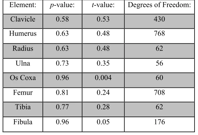
regression models were created using only the left elements, Student’s t-tests were employed to demonstrate that there was no significant difference between left and right elements in the
reference sample. The regression models were calculated in Statistical Package for the Social
Sciences 19.0.0. The prediction interval and two-tailed t-distribution were calculated in Microsoft Excel. Student’s t-tests were calculated using the GraphPad Software
CHAPTER 5: Results
Model One Results
Model one compared left and right elements, and considers shape. The elements that
were tested with model one were the clavicle, humerus, radius, ulna, os coxa, femur, tibia
and fibula. Each table represents the results for left and right sides for an element. Each row
and column represents a single element. The p-values for bone pairs that could not be
segregated are highlighted in red.
Table 5.1 presents the results for the clavicle, using Model one. Thirty comparisons
between left (n=5) and right (n=6) clavicles were made. Of these 30 comparisons, 21
possible pairs were differentiated.
Table 5.2 presents the results for the humerus, using model one. Sixty comparisons
between left (n=7) and right (n=9) humeri were made. Of the 60 comparisons, 19 possible
pairs were differentiated. In this case, three comparisons were not made. In an attempt to be
conservative, any two humeri that exhibited a difference of 10 or more millimeters in
maximum length, were not tested against each other (Auerbach and Ruff 2006; LeGarde
2012). In Table 5.2, these three pairs are denoted with NT, for “not tested.”
Table 5.3 presents the results for the radius, using model one. Eighty-eight
comparisons between left (n=11) and right (n=8) radii were made. Of the 88 comparisons, 37
possible pairs were segregated.
Table 5.4 reports the results for the ulna, using model one. Eighty comparisons
pairs were segregated. Seven pairs were not tested against each other due to differences in
maximum length (Auerbach and Ruff 2006); these will be denoted in Table 5.4 as NT, for
“not tested.”
Table 5.5 reports the results for the os coxa, using model one. Forty-two comparisons
between left (n=7) and right (n=6) os coxae were made. Of the 42 comparisons, 27 possible
pairs were differentiated.
Table 5.6 presents the results for the femur, using model one. Forty-eight
comparisons between left (n=6) and right (n=8) os coxae were made. Of the 48 comparisons,
22 of the possible pairs were isolated. Eleven pairs were not tested against each other due to
glaring differences in maximum length (Auerbach and Ruff 2006); these will be denoted in
Table 5.5 as NT, for “not tested.”
Table 5.7 reports the results for the tibia, using model one. Sixty-four comparisons
`between left (n=8) and right (n=8) tibiae were made. Of the 64 comparisons, 27 of the
possible pairs were isolated. Twelve pairs were not tested against each other due to sizeable
differences in maximum length (Auerbach and Ruff 2006); these will be denoted in Table 5.6
Table 5.1 Results for Model 1: Clavicle
Table 5.2 Results for Model 1: Humerus
Table 5.3 Results for Model 1: Radius
Table 5.4 Results for Model 1: Ulna
583.1 1147.2 1147.1 1336.1 335.1 335.2
583.2 0.269 0.000 0.006 0.000 0.000 0.000
1337.1 0.000 0.046 0.929 0.001 0.001 0.128
582 0.000 0.000 0.030 0.612 0.530 0.180
1150.1 0.024 0.000 0.030 0.387 0.455 0.007
340.1 0.000 0.021 0.339 0.000 0.000 0.000
Left Clavicles Ri ght Cl avi cl es
657.2 657.1 1081.2 1081.1 1081.3 1082.2 341.1
658.2 0.000 0.005 0.001 NT 0.640 0.735 0.585
658.1 0.097 0.516 0.299 NT 0.735 0.069 0.677
1079.2 0.203 0.126 0.052 0.876 0.467 0.755 0.516
1079.1 0.299 0.194 0.087 0.203 0.621 0.755 0.677
1078.1 0.000 0.000 0.000 0.640 0.242 0.000 0.213
1078.3 0.213 0.815 0.324 NT 0.132 0.026 0.113
415.3 0.000 0.000 0.000 0.010 0.795 0.041 0.856
415.2 0.020 0.113 0.350 0.000 0.533 0.533 0.533
415.1 0.795 0.436 0.876 0.735 0.451 0.856 0.677
Ri ght H um eri Left Humeri
639.3 639.1 1071.2 1071.1 1071.4 1071.6 1071.5 1071.3 416.3 416.1 346 639.2 0.900 0.490 0.012 0.014 0.010 0.034 0.510 0.025 0.062 0.777 0.122 639.4 0.020 0.070 0.102 0.000 0.875 0.225 0.753 0.182 0.348 0.777 0.000 1070.1 0.018 0.004 0.004 0.398 0.000 0.011 0.262 0.034 0.146 0.753 0.433 1070.2 0.062 0.182 0.004 0.000 0.900 0.011 0.262 0.062 0.022 0.550 0.001 1368.1 0.348 0.753 0.004 0.182 0.192 0.012 0.192 0.024 0.010 0.332 0.706 410.1 0.014 0.051 0.075 0.000 0.682 0.172 0.875 0.085 0.275 0.593 0.000 410.2 0.080 0.020 0.753 0.172 0.163 0.925 0.163 0.801 0.975 0.729 0.004 410.3 0.801 0.381 0.070 0.875 0.900 0.154 0.900 0.122 0.137 0.572 0.122
Left Radii Ri ght Ra di i
659 1095.3 1370.1 1370.2 455 446.3 446.1 446.2
660 0.000 0.765 0.691 0.384 NT 0.000 0.000 0.619
1094.4 0.564 0.512 0.182 0.765 0.405 0.000 0.538 0.512
1094.1 0.063 0.066 0.014 0.578 0.106 0.000 0.858 0.056
1094.3 0.405 0.873 0.591 0.269 0.691 0.000 0.921 0.647
1094.6 0.081 0.137 0.058 0.475 0.052 0.043 0.223 0.153
1094.7 0.705 NT NT NT 0.796 0.827 0.676 NT
1094.5 0.811 0.765 0.691 0.384 0.633 0.676 0.720 0.765
1094.2 0.705 0.905 0.705 NT 0.691 0.796 NT 0.858
427.1 0.087 0.342 0.170 0.705 0.058 0.081 0.416 0.287
427.2 0.269 0.780 0.475 0.605 0.195 0.253 0.858 0.662