A version of this paper appears inConferences in Research and Practice in Information Technology(CRPIT), volume 98, pages 7–19, Ljiljana Brankovic and Willy Susilo ed., ACS, 2009.
Faster Group Operations on Elliptic Curves
Huseyin Hisil, Kenneth Koon-Ho Wong, Gary Carter, Ed Dawson
Information Security Institute, Queensland University of Technology,
Brisbane, QLD, Australia, 4000
{h.hisil, kk.wong, g.carter, e.dawson}@qut.edu.au
Abstract
This paper improves implementation techniques of Elliptic Curve Cryptography. We introduce new formulae and algorithms for the group law on Jacobi quartic, Jacobi intersection, Edwards, and Hessian curves. The proposed formulae and algorithms can save time in suitable point representations. To support our claims, a cost comparison is made with classic scalar multiplication algorithms using previous and current operation counts. Most notably, the best speedup is obtained in the case of Jacobi quartic curves which also lead to one of the most efficient scalar multiplications benefiting from the proposed2M+ 5S+ 1D(i.e. 2 multiplications, 5 squarings, and 1 multiplication by a curve constant) point doubling and7M+3S+1Dpoint addition algorithms. Furthermore, the new addition algorithm provides an efficient way to protect against side channel attacks which are based on simple power analysis (SPA).
Keywords:Efficient elliptic curve arithmetic, unified addition, side channel attack.
1
Introduction
From the advent of elliptic curve cryptosystems, in-dependently by Miller (1986) and Koblitz (1987) to date, the arithmetic of elliptic curves has drawn wide attention from cryptographic researchers. It is well known that the Weierstrass model provides a general parametrization of elliptic curves. In other words, an elliptic curve over a field K (excluding char(K) = 2,3) is the set of points(x, y)satisfying the equation
y2
=x3
+ax+b
for some a, b ∈ K where 4a3
+ 27b2
6
= 0 together with the point at infinity O. These points exhibit a group structure under an explicitly defined additive group law. In other words, two points P = (x1, y1) andQ = (x2, y2)can be added to form a third point R=P+Q= (x3, y3)on the same curve. The
nega-tive of the pointP is(x1,−y1). The identity element
is the point at infinityO. From this we can define a scalar multipleSof a pointP as
S= [k]P=P+P+. . .+P
| {z }
ktimes .
Computing k when only P and S are known is be-lieved to be intractable for carefully selected param-eters. This forms the basis of the elliptic curve dis-crete logarithm problem, which is used to provide cryptographic security.
One of the main challenges in elliptic curve cryp-tography is to perform scalar multiplication effi-ciently under different environmental constraints (such as resistance to side channel attacks, band-width efficiency, memory limitations). In this paper, we restrict attention to the optimization of point addi-tion and point doubling which are vital for the overall performance of double-and-add type scalar multipli-cation algorithms.
Elliptic curves can be represented in several differ-ent ways. To obtain faster group operations, some other elliptic curve representations have also been considered in the last two decades. In this context, we present a short outline of previous work on which our paper is built.
intersec-tion, and Hessian curves.
- Cohen et al. (1998) provided efficient strategies for scalar multiplication on Weierstrass curves. Doche et al. (2006) introduced fast doubling and tripling algorithms on Weierstrass curves for two special families. The doubling algorithm in (Doche et al. 2006) was improved by Bernstein et al. (2007) forS<M.
- In chronological order, Joye & Quisquater (2001), Liardet & Smart (2001), Brier & Joye (2002), Billet & Joye (2003) showed ways of perform-ing scalar multiplication with resistance to side channel attacks using Hessian, Jacobi intersec-tion, Weierstrass and Jacobi quartic forms, re-spectively.
- Duquesne (2007) proposed a faster algorithm for computing point addition on Jacobi quartic curves based on the formulae in (Billet & Joye 2003) by using an alternative coordinate sys-tem. In (Bernstein & Lange 2007b) and (Bern-stein & Lange 2007a) a better operation count forS<Mwas proposed. Some of the optimiza-tions in this paper benefit from similar ideas.
- Bernstein & Lange (2007c) introduced Edwards curves for providing fast arithmetic and efficient countermeasures to side channel attacks. Later, Bernstein & Lange (2007d) proposed the in-verted Edwards coordinates which improve tim-ings for Edwards curves and provided the fastest unified addition of that time. Bernstein & Lange (2007b) have built a database of explicit formu-lae that are reported in the literature together with their own optimizations.
For security considerations, the selected curves should have a small cofactor, typically equal to or less than 4. It is possible to find cryptographically in-teresting curves which satisfy the security criterion and which can be parameterized by one of the curve models mentioned above. See (Liardet & Smart 2001), (Billet & Joye 2003), and (Bernstein & Lange 2007c) for sample curves.
In this work, we aim to speedup the group oper-ations for these curves with a final aim of improv-ing the best timimprov-ings for various scalar multiplication algorithms. We extend the literature by introducing new addition and doubling formulae for various curve models. An extensive speed comparison is given in the appendix. From the comparison tables it can be observed that most of our optimizations achieve the removal of field multiplications and/or field squar-ings in comparison to the current literature. In addi-tion, we provideS-Mtradeoffs for the doubling oper-ations.
In what follows we will frequently use the terms unified addition,readdition, andmixed addition. Uni-fied addition means that addition formulae remain valid when two input points are same, see (Cohen et al. 2005, Section 29.1.2). Readdition means that a point addition has already taken place and some of the previously computed data is cached, see (Co-hen et al. 1998) or (Bernstein & Lange 2007c, p.40). Mixed addition means that one of the addends is given in affine coordinates, see (Cohen et al. 1998).
The paper is organized as follows. We provide new formulae and better operation counts for various el-liptic curve forms in Section 2. A naming of different systems are pointed in Section 3. The exceptional cases are considered in Section 4. We make compar-isons of various systems and draw our conclusions in Section 5.
2
Improvements
In the rest of this paper, we assumeKis finite, is of large size, andchar(K)6= 2,3. For any elliptic curve over K we restrict our attention to the K-rational points. Not all of these assumptions are always nec-essary. However, they make our investigation eas-ier. We omit the operation counts for affine coordi-nates since known formulae for this representation require field inversions which are very costly in most implementations compared to field multiplications. We also omit the cost of additions, subtractions, and multiplication by very small constants (e.g. 2, 4, etc.). However, they can be properly counted from the provided algorithms if they are not negligible.
Some of the derivations in this section are aided by the use of (Monagan & Pearce 2006) simplifica-tion algorithms for rasimplifica-tional expressions. We also use computer aid with Maple v.111computer algebra sys-tem. We obtain curve definitions and affine versions of various formulae from (Bernstein & Lange 2007b). We borrow the notationM,S, andDfrom (Bernstein & Lange 2007c).
2.1
Jacobi quartic form
The uses of these curves in cryptology are explained by Chudnovsky & Chudnovsky (1986) and Billet & Joye (2003). A Jacobi quartic form elliptic curve over
Kis defined byy2
=x4
+ 2ax2
+ 1wherea∈Kwith
a2
6
= 1. Birational maps between Weierstrass and Jacobi quartic curves can be found in (Billet & Joye 2003), (Bernstein & Lange 2007b), and (Bernstein & Lange 2007a).
Our main focus in this work is the group law. There-fore we are interested in explicit formulae which add
two points. We use the common notation
(x3, y3) = (x1, y1) + (x2, y2)
which is used in many textbooks. Here(x1, y1) and (x2, y2)are the addends and(x3, y3)is the sum.
The explicit formulae for the group law on Ja-cobi quartic form elliptic curves date back to (JaJa-cobi 1829). Even earlier, a formula for computingx3(see
below in (1)) appears in one of Euler’s works from the 18th
century, (Euler 1761). A formula for computing
y3 can be found in (McKean & Moll 1927, p.111). We
will proceed with working on the affine version of the unified addition formulae in (Billet & Joye 2003) given by
(x3, y3) = (x1, y1) + (x2, y2)
where
x3 =
x1y2+y1x2
1−x21x 2 2
,
y3 =
(y1y2+ 2ax1x2)(x 2 1x
2
2+ 1) + 2x1x2(x 2 1+x
2 2)
(1−x21x 2 2)
2 .
(1) The identity element is the point (0,1). The neg-ative of a point(x, y) is(−x, y). In this section, we will update the numerator ofy3. If the numerator is
designatedtthen we have
t = (y1y2+ 2ax1x2)(x 2 1x
2
2+ 1) + 2x1x2(x 2 1+x
2 2)
= (y1y2+ 2ax1x2)(x 2 1x
2
2+ 1) + 2x1x2(x 2 1+x
2 2) +
x2 1y
2
2+ 2x1y1x2y2+y 2 1x
2
2−(x1y2+y1x2) 2
.
Using the curve equationy2
= x4
+ 2ax2
+ 1, we replacey2
1withx 4 1+ 2ax
2
1+ 1andy 2 2withx
4 2+ 2ax
2 2+ 1.
This yields
t = (y1y2+ 2ax1x2)(x 2 1x
2
2+ 1) + 2x1x2(x 2 1+x
2 2) +
x21(x 4 2+ 2ax
2
2+ 1) + 2x1y1x2y2+
x22(x 4 1+ 2ax
2
1+ 1)−(x1y2+y1x2) 2
.
We obtain the new formula fory3by organizing the
terms. The new unified addition formulae are given by
(x3, y3) = (x1, y1) + (x2, y2)
where
x3 =
x1y2+y1x2
1−x21x 2 2
,
y3 =
x1x2+ 1
1−x21x 2 2
2
(x21+ 1)(x 2 2+ 1) +
y1y2+ (2a−2)x1x2
−x
2 3−1.
(2) A projective weighted coordinate systems is used in (Chudnovsky & Chudnovsky 1986) and in (Billet & Joye 2003) for the elimination of field inversions. In this system, each point is represented by the triplet (X:Y:Z) which satisfies the equation Y2
=
X4
+2aX2 Z2
+Z4
and corresponds to the affine point
(X/Z, Y /Z2
) with Z 6= 0. The identity element is represented by(0: 1: 1). The negative of(X:Y:Z)is (−X:Y:Z). The new point addition (2) in projective weighted coordinates then becomes
(X3:Y3:Z3) = (X1:Y1:Z1) + (X2:Y2:Z2)
where
X3 = X1Z1Y2+Y1X2Z2,
Z3 = Z 2 1Z
2 2−X
2 1X
2 2,
Y3 = (X1X2+Z1Z2) 2
((X2 1 +Z
2 1)(X
2 2 +Z
2 2) +
Y1Y2+ (2a−2)X1Z1X2Z2)−X 2 3 −Z
2 3.
(3) Rather than using the projective weighted coordi-nates, we use a redundant representation of points for efficiency purposes. This representation is based on the work of Duquesne (2007) which is extended in (Bernstein & Lange 2007a).
We represent a point with Z 6= 0 with the sextuplet (X:Y:Z:X2
:Z2
:XZ) and incorpo-rate this representation with the new point addi-tion formulae (3). Now, (X1:Y1:Z1:U1:V1:W1) and
(X2:Y2:Z2:U2:V2:W2)withU1=X12,V1 =Z12,W1= X1Z1,U2 =X22,V2 =Z22,W2 =X2Z2 can be added
with the algorithm
A←U1U2, B←V1V2, C←W1W2, D←Y1Y2,
X3←(W1+Y1)(W2+Y2)−C−D, Z3←B−A,
U3←X 2
3, V3←Z 2
3, F ←A+B+ 2C,
G←(U1+V1)(U2+V2) +kC+D, H←U3+V3,
Y3←F G−H, W3←((X3+Z3) 2
−H)/2
wherek = 2(a−1). The new unified addition costs 7M+ 3S+ 1Din the modified coordinates. Assum-ing that (X2:Y2:Z2:U2:V2:W2) is cached, a
readdi-tion costs7M+ 3S+ 1D. A6M+ 3S+ 1Dmixed ad-dition can be derived by settingZ2 = 1. We use the name “modified Jacobi quartic v.2b” to refer to this coordinate system. Modified Jacobi quartic v.2b uses the new addition formulae and a 3M+ 4S doubling algorithm proposed by Hisil et al. (2007).
To evaluate the new addition formulae, a similar algorithm for a less redundant version of modified Jacobi quartic v.2b which represents points with the quintuplet (X:Y:Z:U:V), is also very efficient in practice. This point representation is proposed in (Hi-sil et al. 2007). In this system the new unified addi-tion costs7M+ 4S+ 1D(by computingW1= ((X1+ Z1)
2
−U1−V1)/2andW2= ((X2+Z2) 2
−U2−V2)/2
on the fly, and not computing W3). Following this
and assuming that(X2:Y2:Z2:U2:V2)is cached, the
readdition costs7M+ 3S+ 1Dwith the extra caching ofW2. A6M+ 3S+ 1Dmixed addition can then be derived by settingZ2 = 1. We use the name
system also uses3M+ 4Sdoubling algorithm in (Hi-sil et al. 2007). A comparison of our results with the literature is given as follows.
Jacobi quartic Addition (Billet & Joye 2003),(ǫ= 1) 10M+3S+1D
(Duquesne 2007),(ǫ= 1) 9M+2S+1D
(Bernstein & Lange 2007b) 8M+3S+1D
This work (modified v.2a) 7M+4S+1D
This work (modified v.2b) 7M+3S+1D
It is convenient here to note that the3M+ 4S dou-bling algorithm in (Hisil et al. 2007) can be easily de-rived from the new affine addition formulae (2) as fol-lows. We symbolically input the same points to the new addition formulae and obtain
(x3, y3) = [2](x1, y1)
where
x3 =
2x1y1
1−x41
,
y3 =
x2 1+ 1
1−x41
2
(x41+ 2ax 2 1+ 1 +y
2 1)−x
2 3−1.
(4) We then replace x4
1 + 2ax 2
1+ 1 withy 2
1 using the
curve equation. This yields
(x3, y3) = [2](x1, y1)
where
x3 =
2x1y1
1−x41
y3 = 2
y1(x 2 1+ 1)
1−x41
2
−x
2 3−1
(5) The point doubling formulae (5) in projective weighted coordinates are given by
(X3:Y3:Z3) = [2](X1:Y1:Z1)
where
X3 = 2X1Y1Z1,
Z3 = Z 4 1 −X
4 1,
Y3 = 2(Y1(X 2 1 +Z
2 1))
2
−X
2 3−Z
2 3.
(6) These formulae are advantageous when used with both versions of the modified coordinates. The point doubling algorithm for (6) is given by
A←U1+V1, X3←2Y1W1, Z3←A(V1−U1),
U3←X32, V3←Z32, B←U3+V3,
W3←((X3+Z3) 2
−B)/2, Y3←2(Y1A) 2
−B.
Doubling costs3M+4Sin both versions of the mod-ified coordinates. See the works (Hisil et al. 2007) and (Bernstein & Lange 2007b).
Building on similar ideas, it is possible to derive the following doubling formulae
(x3, y3) = [2](x1, y1)
where
x3 =
2x1y1
1−x41
,
y3 = 2
y2 1
1−x41
2
−ax
2 3−1.
(7) The new doubling formulae in projective weighted coordinates are given by
(X3:Y3:Z3) = [2](X1:Y1:Z1)
where
X3 = 2X1Y1Z1,
Z3 = Z 4 1−X
4 1,
Y3 = 2Y 4 1 −aX
2 3−Z
2 3.
(8) These formulae are again advantageous when used with both versions of the modified coordi-nates. We reproduce both versions of the modified coordinates with the names “modified Jacobi quar-tic v.3a” and “modified Jacobi quarquar-tic v3.b” to em-phasize the use of the new doubling formulae to-gether with the new addition formulae (3). A point (X1:Y1:Z1:U1:V1:W1)can be doubled with the
algo-rithm
X3←2Y1W1, Z3←(V1−U1)(V1+U1), U3←X 2 3,
V3←Z 2
3, W3←((X3+Z3) 2
−U3−V3)/2,
Y3←2Y 4
1 −aU3−V3.
Doubling costs2M+ 5S+ 1Din both versions of the modified coordinates. A comparison of our results with the literature is given as follows. The operation counts from the first three entries are from (Bernstein & Lange 2007b).
Jacobi quartic Doubling Bernstein/Lange “dbl-2007-bl” 1M+9S+1D
Hisil/Carter/Dawson “dbl-2007-hcd” 2M+6S+2D
Feng/Wu “dbl-2007-fw-4” 8S+3D
(Hisil et al. 2007) 3M+4S
This work 2M+5S+1D
2.2
Jacobi intersection form
The uses of these curves in cryptology are explained by Chudnovsky & Chudnovsky (1986) and Liardet & Smart (2001). The explicit formulae for the group law date back to (Jacobi 1829). A Jacobi intersection form elliptic curve overKis defined by
s2
+c2
= 1
as2
+d2
= 1
where a ∈ K with a(1 −a) 6= 0. Birational maps between Weierstrass and Jacobi intersection curves can be found in (Liardet & Smart 2001), (Bernstein & Lange 2007b), and (Bernstein & Lange 2007a). Fol-lowing the notation of (Chudnovsky & Chudnovsky 1986), the affine version of the unified addition for-mulae are given by
(s3, c3, d3) = (s1, c1, d1) + (s2, c2, d2)
where
s3 =
s1c2d2+c1d1s2
c2 2+d
2 1s
2 2
,
c3 =
c1c2−s1d1s2d2
c2 2+d
2 1s
2 2
,
d3 =
d1d2−as1c1s2c2
c2 2+d
2 1s
2 2
.
(9) The identity element is the point(0,1,1). The neg-ative of a point (s, c, d) is(−s, c, d). Chudnovsky & Chudnovsky (1986) use projective homogenous co-ordinates to eliminate field inversions. In this sys-tem, each point is represented by the quadruplet (S:C:D:T)which satisfies the equationsS2
+C2
=
T2
and aS2
+D2
= T2
simultaneously and corre-sponds to the affine point(S/T, C/T, D/T)withT 6= 0. The identity element is represented by(0: 1: 1: 1). The negative of (S:C:D:T) is (−S:C:D:T). The point addition (9) in projective homogenous coordi-nates is given by
(S3:C3:D3:T3) = (S1:C1:D1:T1) + (S2:C2:D2:T2)
where
S3 = S1T1C2D2+C1D1S2T2,
C3 = C1T1C2T2−S1D1S2D2,
D3 = D1T1D2T2−aS1C1S2C2,
T3 = D 2 1S
2 2+T
2 1C
2 2.
(10) To eliminate several field multiplications, we modify the homogenous projective coordinates where each point is represented by the sextuplet, (S:C:D:T:SC:DT). The points represented by (S1:C1:D1:T1:U1:V1)and(S2:C2:D2:T2:U2:V2)with
U1=S1C1,V1=D1T1,U2=S2C2,V2=D2T2can be added with the algorithm
E←S1D2, F ←C1T2, G←D1S2, H←T1C2,
J←U1V2, K←V1U2,
S3←(H+F)(E+G)−J−K,
C3←(H+E)(F−G)−J+K,
D3←(V1−aU1)(U2+V2) +aJ−K,
T3←(H+G) 2
−2K, U3←S3C3, V3←D3T3.
The unified point addition costs 11M + 1S + 2D in the modified coordinates. Assuming that (S2:C2:D2:T2:U2:V2)is cached, the readdition costs 11M+ 1S+ 2D. A10M+ 1S+ 2Dmixed addition is easily derived by setting T2 = 1. We use the name
“modified Jacobi intersection” to refer to this system. A similar algorithm can be used for projective ho-mogenous coordinates. The unified addition costs 13M+ 1S+ 2D computingU1 = S1C1, V1 = D1T1, U2 = S2C2, V2 = D2T2 on the fly, and not
com-puting U3 and V3. Following this and assuming
that (S2:C2:D2:T2) is cached, the readdition costs
11M+ 1S+ 2Dwith the extra caching ofU2andV2. A10M+ 1S+ 2Dmixed addition is then derived by settingT2= 1. We use the name “Jacobi intersection v.2” to refer to this system which uses the new addi-tion algorithm. A comparison of our results with the literature is given as follows.
Jacobi intersection Addition (Chudnovsky & Chudnovsky 1986) 14M+2S+1D
(Liardet & Smart 2001) 13M+2S+1D
This work (projective) 13M+1S+2D
This work (modified) 11M+1S+2D
Efficient doubling formulae for the modified Jacobi intersection coordinates can be derived starting from the unified addition formulae (10). We symbolically input the same points into the original addition for-mulae and obtain
(s3, c3, d3) = [2](s1, c1, d1)
where
s3 =
2s1c1d1
c2 1+s
2 1d
2 1
,
c3 =
c2 1−s21d
2 1
c2 1+s
2 1d
2 1
,
d3 =
d2 1−as21c
2 1
c2 1+s
2 1d
2 1
.
(11) Using the defining equations,s2
+c2
= 1andas2
+
d2
= 1, we replacec2 1 withc
2 1(as
2 1+d
2
1)(only for the
denominators) ands2 1d2
1with(1−c 2 1)d
2
1. This yields
s3 = (2s1c1d1)/(c 2 1(as
2 1+d
2
1) + (1−c
2 1)d
c3 = (c 2 1(as
2 1+d
2
1)−(1−c
2 1)d
2 1)/
(c2 1(as
2 1+d
2
1) + (1−c
2 1)d
2 1),
d3 = (d 2 1−as
2 1c
2 1)/(c
2 1(as
2 1+d
2
1) + (1−c
2 1)d
2 1).
These substitutions give an intermediate formula forc3where
s3 = (2s1c1d1)/(d 2 1+as
2 1c
2 1),
c3 = (as 2 1c
2 1+ 2c
2 1d
2 1−d
2 1)/(d
2 1+as
2 1c
2 1),
d3 = (d 2 1−as
2 1c
2 1)/(d
2 1+as
2 1c
2 1).
Finally, we replace2c2 1d2
1 with2c 2 1(s
2 1+c
2 1−as
2 1)in c3.
s3 = (2s1c1d1)/(as 2 1c
2 1+d
2 1),
c3 = (as 2 1c
2 1+ 2c
2 1(s
2 1+c
2 1−as
2 1)−d
2 1)/(as
2 1c
2 1+d
2 1),
d3 = (d 2 1−as21c
2 1)/(as
2 1c
2 1+d
2 1).
The new following doubling formulae are given by
(s3, c3, d3) = [2](s1, c1, d1)
where
s3 =
2s1c1d1
d2 1+as
2 1c
2 1
,
c3 = −
d2 1−as21c
2 1+ 2(s
2 1c
2 1+c
4 1)
d2 1+as
2 1c
2 1
,
d3 =
d2 1−as21c
2 1
d2 1+as
2 1c 2 1 . (12) The new doubling formulae (12) in projective ho-mogenous coordinates are given by
(S3:C3:D3:T3) = [2](S1:C1:D1:T1)
where
S3 = 2S1C1D1T1,
C3 = −D 2 1T
2 1 −aS
2 1C
2 1+ 2(S
2 1C
2 1+C
4 1),
D3 = D 2 1T
2 1 −aS
2 1C
2 1,
T3 = D 2 1T
2 1 +aS
2 1C
2 1.
(13) Now, (S1:C1:D1:T1:U1:V1) can be doubled with
the algorithm
E←V12, F ←U12, G←aF, T3←E+G,
D3←E−G, C3←2(F+C 4 1)−T3,
S3←(U1+V1) 2
−E−F, U3←S3C3, V3←D3T3.
It is easy to see that point doubling costs 2M+ 5S+1Dboth on projective homogenous and modified projective homogenous coordinates. A comparison of our results with the literature is given as follows.
Jacobi intersection Doubling (Liardet & Smart 2001) 4M+3S
(Bernstein & Lange 2007b) 3M+4S
This work 2M+5S+1D
2.3
Edwards form
The uses of these curves in cryptology are ex-plained by Bernstein & Lange (2007c), Bernstein et al. (2007), and Bernstein & Lange (2007d). An Ed-wards form elliptic curve overK is defined by x2
+
y2
=c2
(1+dx2 y2
)wherec, d∈Kwithcd(1−c4 d)6= 0. Birational maps between Weierstrass and Edwards curves are given by (Bernstein & Lange 2007c). The affine unified addition formulae are given by
(x3, y3) = (x1, y1) + (x2, y2)
where
x3 =
x1y2+y1x2
c(1 +dx1y1x2y2)
,
y3 =
y1y2−x1x2
c(1−dx1y1x2y2)
.
(14) The identity element is the point (0, c). The neg-ative of a point (x, y) is (−x, y). We first describe how new addition formulae for Edwards curves can be derived from the original addition formulae in (Bernstein & Lange 2007c). Consider the relations
x2 1+y
2 1−c
2
(1 +dx2 1y2
1) = 0,x 2 2+y
2 2−c
2
(1 +dx2 2y2
2) = 0
obtained from the curve equation. From this, we can expresscanddin terms ofx1, x2, y1, y2as follows.
c2 = x 2 1x 2 2y 2 1−x21x
2 2y
2 2+x
2 1y
2 1y
2 2−x22y
2 1y 2 2 x2 1y 2 1−x
2 2y
2 2
,
d = x
2 1−x
2 2+y
2 1−y
2 2 x2 1x 2 2y 2 1−x
2 1x
2 2y
2 2+x
2 1y
2 1y
2 2−x
2 2y 2 1y 2 2 .
Substitutions can be made in the original addition formulae to obtain
x3 = (x1y2+y1x2)/((1/c)(x 2 1x
2 2y
2 1−x
2 1x
2 2y
2 2+x
2 1y 2 1y 2 2− x2 2y 2 1y 2 2)/(x
2 1y
2 1−x
2 2y
2 2)(1 + (x
2 1−x
2 2+y
2 1−y
2 2)/
(x2 1x
2 2y
2 1−x
2 1x
2 2y
2 2+x
2 1y
2 1y
2 2−x
2 2y
2 1y
2
2)x1y1x2y2)),
y3 = (y1y2−x1x2)/((1/c)(x 2 1x
2 2y
2 1−x
2 1x
2 2y
2 2+x
2 1y 2 1y 2 2− x2 2y 2 1y 2 2)/(x
2 1y
2 1−x
2 2y
2 2)(1−(x
2 1−x
2 2+y
2 1−y
2 2)/
(x2 1x
2 2y
2 1−x21x
2 2y
2 2+x
2 1y
2 1y
2 2−x22y
2 1y
2
2)x1y1x2y2)).
After straightforward simplifications, the new addi-tion formulae are given by
(x3, y3) = (x1, y1) + (x2, y2)
where
x3 =
c(x1y1+x2y2)
x1x2+y1y2
,
y3 =
c(x1y1−x2y2)
x1y2−y1x2
.
formulae show an interesting fact that dedicated ad-dition on the Edwards curves does not depend on the curve parameterd. Therefore, arbitrary selections of
ddo not cause any efficiency loss.
Bernstein & Lange (2007c) use homogenous pro-jective coordinates to prevent field inversions that appear in the affine formulae. We also represent each point in projective homogenous coordinates for the new formulae (15). Each point is represented by the triplet(X:Y:Z)which satisfies the projective curve (X2
+Y2
)Z2
= c2
(Z4
+dX2 Y2
) and corre-sponds to the affine point (X/Z, Y /Z) with Z 6= 0. The identity element is represented by(0 :c: 1). The negative of(X:Y:Z) is (−X:Y:Z). The new addi-tion formulae in projective homogenous coordinates are given by
(X3:Y3:Z3) = (X1:Y1:Z1) + (X2:Y2:Z2)
where
X3 = Z1Z2(X1Y2−Y1X2)(X1Y1Z 2 2+Z
2 1X2Y2),
Y3 = Z1Z2(X1X2+Y1Y2)(X1Y1Z 2
2−Z12X2Y2),
Z3 = kZ 2 1Z
2
2(X1X2+Y1Y2)(X1Y2−Y1X2)
(16) withk= 1/c. Now,(X1:Y1:Z1)and (X2:Y2:Z2)can
be added with the algorithm
A←X1Z2, B←Y1Z2, C←Z1X2, D←Z1Y2,
E←AB, F ←CD, G←E+F, H←E−F,
J←(A−C)(B+D)−H, K←(A+D)(B+C)−G,
X3←GJ, Y3←HK, Z3←k JK.
We also investigate the case for inverted Ed-wards coordinates introduced by Bernstein & Lange (2007d). In this system, each triplet(X:Y:Z) satis-fies the curve(X2
+Y2
)Z2
=c2
(dZ4
+X2 Y2
)and cor-responds to the affine point(Z/X, Z/Y)withXY Z6= 0. The identity element is represented by the vector (c,0,0). The negative of(X:Y:Z)is(−X:Y:Z). The new addition formulae (15) in inverted Edwards coor-dinates are given by
(X3:Y3:Z3) = (X1:Y1:Z1) + (X2:Y2:Z2)
where
X3 = Z1Z2(X1X2+Y1Y2)(X1Y1Z 2 2−Z
2 1X2Y2),
Y3 = Z1Z2(X1Y2−Y1X2)(X1Y1Z 2 2+Z
2 1X2Y2),
Z3 = c(X1Y1Z 2 2+Z
2
1X2Y2)(X1Y1Z 2 2−Z
2 1X2Y2).
(17) (X1:Y1:Z1)and(X2:Y2:Z2)can be added with the
algorithm
A←X1Z2, B←Y1Z2, C←Z1X2, D←Z1Y2,
E←AB, F ←CD, G←E+F, H←E−F,
X3←((A+D)(B+C)−G)H,
Y3←((A−C)(B+D)−H)G, Z3←c GH.
A detail to mention is the readdition in projective homogenous coordinates. At this stage, it is more convenient to divide each coordinate of the new for-mulae (16) by Z1Z2. The readdition of (X2:Y2:Z2) can then be performed with the cached valuesR1= X2Y2andR2=Z22using the algorithm
A←X1Y1, B←Z 2
1, C←R2A, D←R1B,
E←(X1−X2)(Y1+Y2)−A+R1,
F←(X1+Y2)(Y1+X2)−A−R1,
G←((Z1+Z2) 2
−B−R2)/2, X3 ←E(C+D),
Y3←F(C−D), Z3 ←k EF G.
In the rest of this section, we assumec = 1. See (Bernstein & Lange 2007c, Section 4). The dedi-cated addition then costs 11M for both coordinate systems. A9Mmixed addition can be derived by set-tingZ2 = 1again for both coordinate systems. The
readdition costs9M+ 2Sin projective homogenous coordinates. A comparison of our results with the lit-erature is given as follows.
Edwards (projective) Addition (Bernstein & Lange 2007c) 10M+1S+1D
This work 11M
Edwards (projective) Readdition (Bernstein & Lange 2007c) 10M+1S+1D
This work 9M+2S
Edwards (projective) Mixed addition (Bernstein & Lange 2007c) 9M+1S+1D
This work 9M
See “Edwards v.2” in Table 1 and Table 2 in the appendix for further comparison.
In fact, the readdition algorithm shows that a modified version of the homogenous projective Ed-wards coordinates in which the points are repre-sented by the quintuplet (X:Y:Z:Z2
:XY) permits an inversion-free addition in9M+ 2Susing the same algorithm. ForS<M, this is faster than the11M al-gorithm that we have just described. However, the 3M+ 4S doubling algorithm in (Bernstein & Lange 2007c) seems to cost5M+ 2Sin this coordinate sys-tem and also the mixed addition costs8M+ 2Swhich is slower than the 9M mixed addition given above. Therefore, we do not further consider this system.
Edwards (inverted) Mixed addition (Bernstein & Lange 2007d) 8M+1S+1D
This work 9M
See “Inverted Edwards v.2” in Table 1 and Table 2 in the appendix.
We also refer the reader to (Bernstein et al. 2008). We should note here that our more recent work (Hisil et al. 2008) which was published before this work, further improves these operation counts on twisted Edwards curves.
2.4
Hessian form
The uses of these curves in cryptology are ex-plained by Chudnovsky & Chudnovsky (1986), Joye & Quisquater (2001), and Smart (2001). An el-liptic curve over K in Hessian form is defined by
x3
+y3
+ 1 = 3dxy whered ∈K withd3
6
= 1. Bira-tional maps between Weierstrass and Hessian curves can be found in (Smart 2001), (Joye & Quisquater 2001), (Bernstein & Lange 2007b), and (Bernstein & Lange 2007a). The addition formulae attributed to Sylvester in (Chudnovsky & Chudnovsky 1986, pp.424-425) are given in (Bernstein & Lange 2007b) by
(x3, y3) = (x1, y1) + (x2, y2)
where
x3 =
y2
1x2−y22x1
x2y2−x1y1
,
y3 =
x2
1y2−x22y1
x2y2−x1y1
.
(18) The identity element is the point at infinity. The negative of a point (x, y) is (y, x). On projective homogenous coordinates, each point is represented by the triplet(X:Y:Z)which satisfies the projective curveX3
+Y3
+Z3
= 3dXY Z and corresponds to the affine point(X/Z, Y /Z)withZ 6= 0. The identity element is represented by(−1: 1: 0). The negative of (X:Y:Z)is(Y:X:Z). The point addition (22) formu-lae (with each coordinate multiplied by 2) in projec-tive homogenous coordinates are given by,
(X3:Y3:Z3) = (X1:Y1:Z1) + (X2:Y2:Z2)
where
X3 = 2Y 2
1X2Z2−2X1Z1Y 2 2,
Y3 = 2X 2
1Y2Z2−2Y1Z1X 2 2,
Z3 = 2Z 2
1X2Y2−2X1Y1Z 2 2.
(19) The point addition algorithms in (Chudnovsky & Chudnovsky 1986) and (Joye & Quisquater 2001) re-quire 12M. To gain speedup in the case S < M, we modify projective homogenous coordinates with a more redundant representation of points using
the nonuplet,(X:Y:Z:X2
:Y2
:Z2
: 2XY: 2XZ: 2Y Z). Two distinct points represented by
(X1:Y1:Z1:R1:S1:T1:U1:V1:W1)
and
(X2:Y2:Z2:R2:S2:T2:U2:V2:W2)
withR1 =X12,S1 =Y12,T1=Z12,U1 = 2X1Y1,V1 =
2X1Z1, W1 = 2Y1Z1, R2 = X22, S2 = Y22, T2 = Z22, U2= 2X2Y2,V2= 2X2Z2,W2= 2Y2Z2can be added
with the algorithm
X3←S1V2−V1S2, Y3←R1W2−W1R2,
Z3←T1U2−U1T2, R3←X 2
3, S3←Y 2
3, T3←Z 2 3,
U3←(X3+Y3) 2
−R3−S3,
V3←(X3+Z3) 2
−R3−T3,
W3←(Y3+Z3) 2
−S3−T3.
The addition2costs6M+6Sin the modified Hessian coordinates. Assuming that
(X2:Y2:Z2:R2:S2:T2:U2:V2:W2)
is cached, the readdition costs6M+ 6S. A5M+ 6S mixed addition can then be derived by settingZ2 =
1. We use the name “modified Hessian” to refer to these results in Section 5. A comparison of our re-sults with the literature is given as follows.
Hessian Addition (Chudnovsky & Chudnovsky 1986) 12M
(Joye & Quisquater 2001) 12M
This work 6M+6S
A similar algorithm can be used for the homoge-nous projective coordinates for the readdition and the mixed addition. Assuming that (X2:Y2:Z2) is cached, the readdition costs 6M + 6S with the ex-tra caching ofR2, S2, T2, U2, V2, W2. A5M+ 6Smixed
addition can be derived by setting Z2 = 1. We use
the name “Hessian v.2” to refer to these results in Section 5. Also see (Hisil et al. 2007, pp.146–147).
For speed oriented implementations, Sylvester’s doubling formulae are given by
(x3, y3) = [2](x1, y1)
where
x3 =
y1(1−x 3 1)
x3 1−y
3 1
,
y3 = −
x1(1−y 3 1)
x3 1−y
3 1
.
(20) 2Point doubling can be performed after a suitable permutation
of coordinates as follows (Z1:X1:Y1:T1:R1:S1:V1:W1:U1)+
(Y1:Z1:X1:S1:T1:R1:W1:U1:V1) using the addition formulae
When working with the modified coordinates, there exists a doubling strategy which requires no addi-tional effort for generating the new coordinates. The doubling formulae (20) (with each coordinate multi-plied by 4) in projective homogenous coordinates are given by
X3 = (2X1Y1−2Y1Z1)(2X1Z1+ 2(X 2 1+Z
2 1)),
Y3 = (2X1Z1−2X1Y1)(2Y1Z1+ 2(Y 2 1 +Z
2 1)),
Z3 = (2Y1Z1−2X1Z1)(2X1Y1+ 2(X 2 1+Y
2 1)).
(21) Now,(X1:Y1:Z1:R1:S1:T1:U1:V1:W1)can be
dou-bled with the algorithm
X3←(U1−W1)(V1+ 2(R1+T1)),
Y3←(V1−U1)(W1+ 2(S1+T1)),
Z3←(W1−V1)(U1+ 2(R1+S1)), R3←X32,
S3←Y 2
3, T3←Z 2
3, U3←(X3+Y3) 2
−R3−S3,
V3←(X3+Z3) 2
−R3−T3,
W3←(Y3+Z3) 2
−S3−T3.
Point doubling costs3M+ 6Sin both homogenous projective and modified projective homogenous co-ordinates. A comparison of our results with the liter-ature is given as follows.
Hessian Doubling (Chudnovsky & Chudnovsky 1986) 6M+3S
(Hisil et al. 2007) 7M+1S
(Hisil et al. 2007) 3M+6S
This work 3M+6S
We comment that it is possible to derive unified addition formulae which do not require any permuta-tions of the coordinates to perform doubling. Assum-ing3x
1x26=y1y2, we multiply the numerator and the
denominator of Sylvester’s addition formulae for x3
by(x3 1x3
2−y 3 1y3
2)and obtain
x3=
(x3 1x
3 2−y31y
3 2)(y
2 1x2−y
2 2x1)
(x3 1x
3 2−y
3 1y
3
2)(x2y2−x1y1)
.
This yields
x3 = (x1y 2 1(y
3 2+x
3 2)(y
2 2y1+x
2 1x2)−
x2y 2 2(y
3 1+x
3 1)(y
2 1y2+x
2 2x1))/
((x31x 3 2−y
3 1y
3
2)(x2y2−x1y1)).
Using the curve equation x2
+y2
+ 1 = 3dxy, the above expression can be rewritten as
x3 = (x1y 2
1(3dx2y2−1)(y 2 2y1+x
2 1x2)−
x2y 2
2(3dx1y1−1)(y 2 1y2+x
2 2x1))/
((x31x 3 2−y
3 1y
3
2)(x2y2−x1y1)).
3This is equivalent to saying(x
1, y1)6=−(x2, y2). The contrary
case should be handled separately as explained in Section 4.
The numerator can be factorized and cancels with (x2y2−x1y1)in the denominator, giving the new
addi-tion formulae. The corresponding formula fory3can be similarly derived from symmetry. We then have
(x3, y3) = (x1, y1) + (x2, y2)
where
x3 =
x1x2(x1y1+x2y2−3dx1x2y1y2) +y 2 1y 2 2 x3 1x 3 2−y
3 1y
3 2
,
y3 = −
y1y2(x1y1+x2y2−3dx1x2y1y2) +x 2 1x 2 2 x3 1x 3 2−y
3 1y 3 2 . (22) The new addition formulae on the projective coor-dinates are given by
X3 = X1X2(X1Y1Z 2
2 +X2Y2Z 2
1−3dX1Y1X2Y2) +
Y12Z1Y 2 2Z2,
Y3 = −Y1Y2(X1Y1Z 2
2+X2Y2Z 2
1−3dX1Y1X2Y2)−
X12Z1X 2 2Z2,
Z3 = X 3 1X
3 2 −Y
3 1Y
3 2.
We again use a modified version of the stan-dard coordinates. Two points(X1:Y1:Z1:V1:W1)and
(X2:Y2:Z2:V2:W2)withV1 = X1Y1, W1 = Z1, V2 2 = X2Y2, W2=Z2
2 can be added with the algorithm
A←X1X2, B←Y1Y2,
C←((Z1+Z2) 2
−W1−W2)/2, D←A 2
, E←B2,
F ←D+E, G←((A+B)2−F)/2,
H ←(V1+W1)(V2+W2)−(3d+ 1)G−C 2
,
X3←AH+EC, Y3← −BH−DC,
Z3←(A−B)(G+F), V3←X3Y3, W3←Z32,
This strategy costs9M+ 6S+ 1D which is faster than the unified addition in Weierstrass form in (Brier & Joye 2002). However, it is slower than all other unified additions considered in this paper. In addi-tion, doubling, readdition and mixed addition formu-lae that can be derived from these formuformu-lae are not attractive. Therefore, we omit these formulae from further comparison with other systems. We are con-tinuing our search to find other unified addition for-mulae which can be faster than the proposed formu-lae.
3
Naming of different systems
4
Handling exceptional cases
An elliptic curve which can be written in one of these forms always has points of small order (other than the identity). The arithmetic of these points can cause division by zero exceptions when affine formu-lae are used. These exceptional cases should be han-dled separately. These cases sometimes require log-ical checks in the projective representations as well.
Cryptographic applications typically use a large prime order subgroup in which these points (except the identity element, O) do not exist. If this is the case, an implementer only needs to be careful about the identity element. When the pointsP andQare to be added, a general strategy to handle the excep-tional cases as follows. LetR be the sum ofP and
Q withP 6= Q. Then, R = QifP = O; R = P if
Q = O; R = O if P = −Q. For all other inputs, the sum can be computed with the relevant formu-lae given in Section 2. Restricting attention to a large prime order subgroup, there are some formulae and coordinate system combinations which do not cause any exception. These are Edwards v.1a, v.1b, Ja-cobi quartic v.1a, v.1b, JaJa-cobi intersection v.1, v.2, modified Jacobi quartic v.1, v.2a, v.2b, v.3a, v.3b and modified Jacobi intersection. Note, for Edwards v.1a and v.1b, the algorithms work for the whole group of points if dis a nonsquare in K. This result is from (Bernstein & Lange 2007c). Again restricting atten-tion to a large prime order subgroup, the systems which need logical checks are inverted Edwards (as explained in (Bernstein & Lange 2007d)) v.1, v.2, Ed-wards v.2, Hessian v.1, v.2, and modified Hessian.
5
Comparison and conclusion
There are several scalar multiplication algorithms which can benefit from the optimizations in this pa-per. We only make comparisons for the popular scalar multiplication strategies using popular elliptic curve parameterizations. We exclude the cost of the final conversion to affine coordinates from our esti-mations.
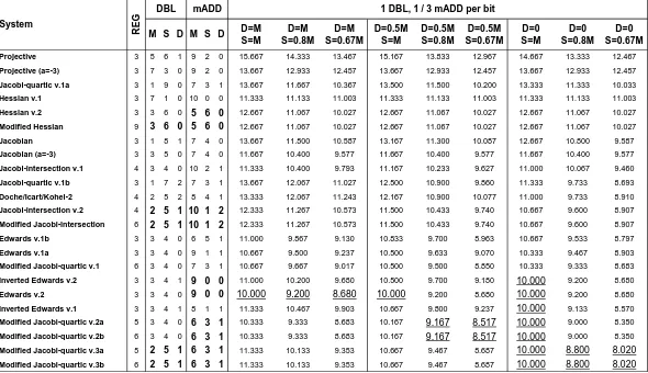
Resource limited environments. In memory limited environments (such as smartcards), there is not enough space for storing precomputation ta-bles. For these environments, scalar multiplication with the “Non-adjacent form without precomputa-tion”method can be a convenient selection. This al-gorithm requires 1 doubling, 1/3 mixed addition per scalar bit. The cost estimates are depicted in Table 1. For example, the best timings for 256-bit scalar multiplication (S/M = 0.8,D/M ≈ 0) are obtained by modified Jacobi quartic v.3a and v.3b which costs approximately2253M. The same operation requires
approximately2662Mfor Weierstrass form(a =−3) using projective weighted (Jacobian) coordinates.
Some points representations such as the modified Hessian coordinates require extra storage for repre-senting each point. This is certainly a disadvantage for space limited applications. However, the primary focus is on the performance in some cases where the processor bandwidth is low.
Speed implementations. This is the most dif-ficult case in which to state a fair comparison be-cause the optimum speeds are somewhat dependent on the choice of the scalar multiplication algorithm. For instance, Doche/Icart/Kohel-3 curves in (Doche et al. 2006) have very fast tripling formulae which can highly benefit from double base number system scalar multiplication. For double-and-add type scalar multiplication algorithms, one might expect to gain the best timing with the system which has the fastest doubling operation since point doubling is the dom-inant operation. However, the readdition and the mixed addition costs also play important roles in the overall timings. We canroughly state that the fast systems forS/M= 0.8,D/M≈0are modified Jacobi quartics v.1, v.2a, v.2b, v.3a, v.3b, inverted Edwards v.1a, v.1b, Edwards v.2, and modified Jacobi intersec-tion. At least, these systems can be very competitive with the Montgomery ladder which has the fixed cost of5M+ 4S+ 1Dper scalar bit in (Montgomery 1987) and4M+ 5S+ 3Din (Castryck et al. 2008) for Mont-gomery curves and3M+ 6S+ 3Din (Gaudry & Lubicz 2008) for Kummer surfaces (the genus 1 case).
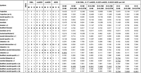
To make the comparison easier, we fix the“signed 4-bit sliding windows”scalar multiplication algorithm analyzed in (Bernstein & Lange 2007c). The al-gorithm requires 0.98 doublings, 0.17 readditions, 0.025 mixed additions and 0.0035 additions per scalar bit for 256-bit scalars. We use this analysis to report current rankings between different systems in Table 2.
With our improvements, either modified Jacobi quartic v.2b or v.3b provides the fastest timings for almost allS/MandD/Mvalues. For example, 256-bit scalar multiplication (S/M = 0.8, D/M ≈ 0) costs approximately1970Mfor modified Jacobi quar-tic v.3a, v.3b. The same operation requires approx-imately 2399Mfor Weierstrass form (a = −3)using projective weighted (Jacobian) coordinates.
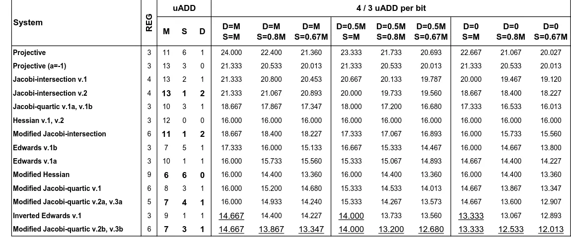
and statistical tools for a successful attack. See Co-hen et al. (2005, Section 29.1.2) as a general refer-ence. This algorithm invokes 4/3 unified additions per scalar bit. The modified coordinates for Hessian and Jacobi intersection forms are only useful here. The7M+ 3S+ 1Dunified addition of modified Jacobi quartic v.2b, v.3b is the fastest among all other uni-fied additions. The cost estimates for various sys-tems are depicted in Table 3.
For example, 256-bit scalar multiplication (S/M= 0.8,D/M ≈ 0) costs approximately 3208M for mod-ified Jacobi quartic v.2b, v.3b. The same operation requires approximately 5257M for Weierstrass form (a=−3)using homogenous projective coordinates.
References
Bernstein, D. J., Birkner, P., Joye, M., Lange, T. & Peters, C. (2008), Twisted Edwards curves, in ‘AFRICACRYPT 2008’, Vol. 5023 ofLNCS, Springer, pp. 389–405.
Bernstein, D. J., Birkner, P., Lange, T. & Peters, C. (2007), Optimizing double-base elliptic-curve single-scalar multiplication, in‘INDOCRYPT 2007’, Vol. 4859 ofLNCS, Springer, pp. 167–182.
Bernstein, D. J. & Lange, T. (2007a), ‘Analysis and op-timization of elliptic-curve single-scalar multiplica-tion’, Cryptology ePrint Archive, Report 2007/455.
http://eprint.iacr.org/.
Bernstein, D. J. & Lange, T. (2007b), ‘Explicit-formulas database’. http://www.hyperelliptic. org/EFD.
Bernstein, D. J. & Lange, T. (2007c), Faster addi-tion and doubling on elliptic curves,in‘ASIACRYPT 2007’, Vol. 4833 ofLNCS, Springer, pp. 29–50.
Bernstein, D. J. & Lange, T. (2007d), Inverted Ed-wards coordinates, in ‘AAECC-17’, Vol. 4851 of LNCS, Springer, pp. 20–27.
Billet, O. & Joye, M. (2003), The Jacobi model of an elliptic curve and side-channel analysis,in ‘AAECC-15’, Vol. 2643 ofLNCS, Springer, pp. 34–42.
Brier, E. & Joye, M. (2002), Weierstraß elliptic curves and side-channel attacks,in‘PKC 2002’, Vol. 2274 ofLNCS, Springer, pp. 335–345.
Castryck, W., Galbraith, S. & Rezaeian Farashahi, R. (2008), ‘Efficient arithmetic on elliptic curves us-ing a mixed Edwards-Montgomery representation’, Cryptology ePrint Archive, Report 2008/218 ver-sion 2008-06-03.http://eprint.iacr.org/.
Chudnovsky, D. V. & Chudnovsky, G. V. (1986), ‘Sequences of numbers generated by addition in formal groups and new primality and factor-ization tests’, Advances in Applied Mathematics 7(4), 385–434.
Cohen, H., Frey, G., Avanzi, R., Doche, C., Lange, T., Nguyen, K. & Vercauteren, F., eds (2005), Hand-book of Elliptic and Hyperelliptic Curve Cryptogra-phy, CRC Press.
Cohen, H., Miyaji, A. & Ono, T. (1998), Efficient ellip-tic curve exponentiation using mixed coordinates, in ‘ASIACRYPT’98’, Vol. 1514 of LNCS, Springer, pp. 51–65.
Doche, C., Icart, T. & Kohel, D. R. (2006), Efficient scalar multiplication by isogeny decompositions,in ‘PKC 2006’, Vol. 3958 ofLNCS, Springer, pp. 191– 206.
Duquesne, S. (2007), ‘Improving the arithmetic of el-liptic curves in the Jacobi model’,Information Pro-cessing Letters104(3), 101–105.
Euler, L. (1761), ‘De integratione aequationis differentialis m dx/√1−x4 = n dy/p1
−y4’, Novi Commentarii Academiae Scientiarum Petropolitanae 6 pp. 37–57. Translated from the Latin by Stacy G. Langton; On the integration of the differential equation
m dx/√1−x4 = n dy/p1
−y4; available at
http://home.sandiego.edu/~langton/eell.pdf.
Gaudry, P. & Lubicz, D. (2008), ‘The arithmetic of characteristic 2 Kummer surfaces’, Cryptology ePrint Archive, Report 2008/133 version 2008-03-25.http://eprint.iacr.org/.
Hisil, H., Carter, G. & Dawson, E. (2007), New for-mulae for efficient elliptic curve arithmetic, in ‘INDOCRYPT 2007’, Vol. 4859 of LNCS, Springer, pp. 138–151.
Hisil, H., Wong, K. K.-H., Carter, G. & Dawson, E. (2008), Twisted Edwards curves revisited, in ‘ASIACRYPT 2008’, Vol. 5350 of LNCS, Springer, pp. 326–343.
Jacobi, C. G. J. (1829), Fundamenta nova theoriae functionum ellipticarum, Sumtibus Fratrum Born-træger.
Joye, M. & Quisquater, J. J. (2001), Hessian elliptic curves and side-channel attacks, in ‘CHES 2001’, Vol. 2162 ofLNCS, Springer, pp. 402–410.
Liardet, P. Y. & Smart, N. P. (2001), Preventing SPA/DPA in ECC systems using the Jacobi form.,in ‘CHES 2001’, Vol. 2162 ofLNCS, Springer, pp. 391– 401.
McKean, H. & Moll, V. (1927), A Course of Modern Analysis, Cambridge University Press.
Miller, V. S. (1986), Use of elliptic curves in cryptog-raphy,in‘CRYPTO’85’, Vol. 218 ofLNCS, Springer, pp. 417–426.
Monagan, M. & Pearce, R. (2006), Rational simplifica-tion modulo a polynomial ideal,in‘ISSAC’06’, ACM, pp. 239–245.
Montgomery, P. L. (1987), ‘Speeding the Pollard and elliptic curve methods of factorization’, Mathemat-ics of Computation48(177), 243–264.
Smart, N. P. (2001), The Hessian form of an elliptic curve,in‘CHES 2001’, Vol. 2162 ofLNCS, Springer, pp. 118–125.
A
Appendix
The appendix is composed of three tables. The un-derlined values are the fastest timings in that col-umn. The rows are sorted with respect to the column (D= 0,S= 0.8M) in descending order. “REG" stands for the number of coordinates in each system. “DBL", “mADD", “reADD", “ADD", and “uADD" stand for the costs of doubling, mixed addition, readdition, addi-tion and unified addiaddi-tion, respectively. Some forms have alternative versions due to alternative opera-tion counts for different S/M andD/M values. It is possible to include more versions due to the rich-ness of current formulae and algorithms. On the other hand, this will decrease readability of the ta-bles. Therefore, we only provide the most significant cases. The references for the comparisons are;
- Doche/Icart/Kohel-2; all operations from (Doche et al. 2006) and (Bernstein & Lange 2007b). The appearance of (Bernstein & Lange 2007b) is to emphasize that faster algorithms are available and are obtained from this database. This is the same for other items in the list.
- Edwards; all operations for v.1a, v.1b, and dou-bling for v.2 from (Bernstein & Lange 2007c).
- Hessian; doubling for v.1, v.2 from (Hisil et al. 2007), readdition, mixed addition, and addition for v.1, addition for v.2 from (Chudnovsky & Chudnovsky 1986).
- Inverted Edwards; all operations for v.1 and dou-bling, readdition and addition for v.2 from (Bern-stein & Lange 2007d).
- Jacobian (a = −3) and Jacobian; all operations from (Chudnovsky & Chudnovsky 1986), (Cohen et al. 1998), and (Bernstein & Lange 2007b).
- Jacobi intersection; doubling, addition, readdi-tion, from (Liardet & Smart 2001) and (Bernstein & Lange 2007b), mixed addition from (Hisil et al. 2007).
- Jacobi quartic; doubling and addition for v.1a, v.1b from (Billet & Joye 2003), (Duquesne 2007), and (Bernstein & Lange 2007b). We note that the2M+6S+2Ddoubling formulae/algorithm by Hisil, Dawson and Carter reported in (Bernstein & Lange 2007b) cost1M+ 7S+ 2Dif the coordi-nateX3is computed as(X1Z1+Y1)2
−(X1Z1)2 − Y2
1. Jacobi quartic; readdition, mixed addition
from (Billet & Joye 2003), (Duquesne 2007), and (Bernstein & Lange 2007b).
- Modified Jacobi quartic; doubling for v.1, v.2a, v.2b (Hisil et al. 2007) and (Bernstein & Lange 2007b), readdition, mixed-addition, and addition for v.1 from (Duquesne 2007) and (Bernstein & Lange 2007b).
- Projective (a = −3) and Projective; doubling, readdition, mixed addition and addition for (Chudnovsky & Chudnovsky 1986) and (Bern-stein & Lange 2007b), unified addition from (Brier & Joye 2002) and (Bernstein & Lange 2007b).
Table 1: Point multiplication cost estimates (inM) per scalar bit of the scalar for “Non-adjacent form without precomputation" method. The underlined values are the fastest timing estimates in that column. The rows are sorted with respect to the column (D= 0,S= 0.8M) in descending order. The new operation counts are given inbold.
M S D M S D D=M S=M
D=M S=0.8M
D=M S=0.67M
D=0.5M S=M
D=0.5M S=0.8M
D=0.5M S=0.67M
D=0 S=M
D=0 S=0.8M
D=0 S=0.67M
Projective 3 5 6 1 9 2 0 15.667 14.333 13.467 15.167 13.833 12.967 14.667 13.333 12.467
Projective (a=-3) 3 7 3 0 9 2 0 13.667 12.933 12.457 13.667 12.933 12.457 13.667 12.933 12.457
Jacobi-quartic v.1a 3 1 9 0 7 3 1 13.667 11.667 10.367 13.500 11.500 10.200 13.333 11.333 10.033
Hessian v.1 3 7 1 0 10 0 0 11.333 11.133 11.003 11.333 11.133 11.003 11.333 11.133 11.003
Hessian v.2 3 3 6 0 5 6 0 12.667 11.067 10.027 12.667 11.067 10.027 12.667 11.067 10.027
Modified Hessian 9 3 6 0 5 6 0 12.667 11.067 10.027 12.667 11.067 10.027 12.667 11.067 10.027
Jacobian 3 1 8 1 7 4 0 13.667 11.800 10.587 13.167 11.300 10.087 12.667 10.800 9.587
Jacobian (a=-3) 3 3 5 0 7 4 0 11.667 10.400 9.577 11.667 10.400 9.577 11.667 10.400 9.577
Jacobi-intersection v.1 4 3 4 0 10 2 1 11.333 10.400 9.793 11.167 10.233 9.627 11.000 10.067 9.460
Jacobi-quartic v.1b 3 1 7 2 7 3 1 13.667 12.067 11.027 12.500 10.900 9.860 11.333 9.733 8.693
Doche/Icart/Kohel-2 4 2 5 2 8 4 1 13.333 12.067 11.243 12.167 10.900 10.077 11.000 9.733 8.910
Jacobi-intersection v.2 4 2 5 1 10 1 2 12.333 11.267 10.573 11.500 10.433 9.740 10.667 9.600 8.907
Modified Jacobi-intersection 6 2 5 1 10 1 2 12.333 11.267 10.573 11.500 10.433 9.740 10.667 9.600 8.907
Edwards v.1b 3 3 4 0 6 5 1 11.000 9.867 9.130 10.833 9.700 8.963 10.667 9.533 8.797
Edwards v.1a 3 3 4 0 9 1 1 10.667 9.800 9.237 10.500 9.633 9.070 10.333 9.467 8.903
Modified Jacobi-quartic v.1 6 3 4 0 7 3 1 10.667 9.667 9.017 10.500 9.500 8.850 10.333 9.333 8.683
Inverted Edwards v.2 3 3 4 1 9 0 0 11.000 10.200 9.680 10.500 9.700 9.180 10.000 9.200 8.680
Edwards v.2 3 3 4 0 9 0 0 10.000 9.200 8.680 10.000 9.200 8.680 10.000 9.200 8.680
Inverted Edwards v.1 3 3 4 1 8 1 1 11.333 10.467 9.903 10.667 9.800 9.237 10.000 9.133 8.570
Modified Jacobi-quartic v.2a 5 3 4 0 6 3 1 10.333 9.333 8.683 10.167 9.167 8.517 10.000 9.000 8.350
Modified Jacobi-quartic v.2b 6 3 4 0 6 3 1 10.333 9.333 8.683 10.167 9.167 8.517 10.000 9.000 8.350
Modified Jacobi-quartic v.3a 5 2 5 1 6 3 1 11.333 10.133 9.353 10.667 9.467 8.687 10.000 8.800 8.020
Modified Jacobi-quartic v.3b 6 2 5 1 6 3 1 11.333 10.133 9.353 10.667 9.467 8.687 10.000 8.800 8.020 1 DBL, 1 / 3 mADD per bit
System
DBL mADD
R
E
G
1
Table 2: Point multiplication cost estimates (inM) per scalar bit of the scalar for “Signed 4-bit Sliding Windows" method with 256 bit scalars. The underlined values are the fastest timing estimates in that column. The rows are sorted with respect to the column (D= 0,S= 0.8M) in descending order. The new operation counts are given inbold.
M S D M S D M S D M S D D=M
S=M
D=M S=0.8M
D=M S=0.67M
D=0.5M S=M
D=0.5M S=0.8M
D=0.5M S=0.67M
D=0 S=M
D=0 S=0.8M
D=0 S=0.67M
Projective 3 5 6 1 12 2 0 9 2 0 12 2 0 14.433 13.177 12.360 13.942 12.685 11.869 13.451 12.194 11.377
Projective (a=-3) 3 7 3 0 12 2 0 9 2 0 12 2 0 12.468 11.801 11.368 12.468 11.801 11.368 12.468 11.801 11.368
Jacobi-quartic v.1a 3 1 9 0 8 3 1 7 3 1 10 3 1 12.136 10.251 9.026 12.039 10.154 8.929 11.942 10.057 8.832
Hessian v.1 3 7 1 0 12 0 0 10 0 0 12 0 0 10.140 9.943 9.816 10.140 9.943 9.816 10.140 9.943 9.816
Jacobian 3 1 8 1 10 4 0 7 4 0 11 5 0 12.475 10.748 9.624 11.984 10.256 9.133 11.493 9.765 8.642
Hessian v.2 3 3 6 0 6 6 0 5 6 0 12 0 0 11.147 9.739 8.824 11.147 9.739 8.824 11.147 9.739 8.824 Modified Hessian 9 3 6 0 6 6 0 5 6 0 6 6 0 11.147 9.735 8.817 11.147 9.735 8.817 11.147 9.735 8.817
Jacobian (a=-3) 3 3 5 0 10 4 0 7 4 0 11 5 0 10.511 9.372 8.632 10.511 9.372 8.632 10.511 9.372 8.632
Doche/Icart/Kohel-2 4 2 5 2 12 5 1 8 4 1 12 5 1 12.213 11.042 10.280 11.134 9.962 9.201 10.054 8.883 8.121
Jacobi-intersection v.1 4 3 4 0 11 2 1 10 2 1 13 2 1 9.577 8.714 8.152 9.480 8.617 8.055 9.383 8.520 7.958
Jacobi-quartic v.1b 3 1 7 2 8 3 1 7 3 1 10 3 1 12.136 10.644 9.675 11.057 9.565 8.595 9.977 8.485 7.516
Edwards v.1b 3 3 4 0 7 5 1 6 5 1 7 5 1 9.376 8.396 7.759 9.279 8.299 7.662 9.182 8.202 7.565
Jacobi-intersection v.2 4 2 5 1 11 1 2 10 1 2 13 1 2 10.560 9.539 8.875 9.874 8.853 8.189 9.189 8.168 7.504
Edwards v.1a 3 3 4 0 10 1 1 9 1 1 10 1 1 9.182 8.357 7.821 9.085 8.260 7.724 8.988 8.163 7.627
Modified Jacobi-intersection 6 2 5 1 11 1 2 10 1 2 11 1 2 10.553 9.531 8.868 9.867 8.846 8.182 9.182 8.161 7.497
Edwards v.2 3 3 4 0 9 2 0 9 0 0 11 0 0 8.963 8.111 7.557 8.963 8.111 7.557 8.963 8.111 7.557
Modified Jacobi-quartic v.1 6 3 4 0 8 3 1 7 3 1 8 3 1 9.182 8.280 7.693 9.085 8.183 7.596 8.988 8.085 7.499
Inverted Edwards v.2 3 3 4 1 9 1 1 9 0 0 9 1 1 9.946 9.126 8.593 9.370 8.550 8.017 8.794 7.974 7.441 Inverted Edwards v.1 3 3 4 1 9 1 1 8 1 1 9 1 1 9.970 9.146 8.609 9.382 8.557 8.021 8.794 7.969 7.433
Modified Jacobi-quartic v.2a 5 3 4 0 7 3 1 6 3 1 7 4 1 8.991 8.088 7.501 8.894 7.991 7.404 8.797 7.894 7.307 Modified Jacobi-quartic v.2b 6 3 4 0 7 3 1 6 3 1 7 3 1 8.988 8.085 7.499 8.891 7.988 7.402 8.794 7.891 7.305 Modified Jacobi-quartic v.3a 5 2 5 1 7 3 1 6 3 1 7 4 1 9.974 8.874 8.159 9.386 8.286 7.571 8.797 7.698 6.983 Modified Jacobi-quartic v.3b 6 2 5 1 7 3 1 6 3 1 7 3 1 9.970 8.871 8.157 9.382 8.283 7.569 8.794 7.695 6.981
0.98 DBL, 0.17 reADD, 0.025 mADD, 0.0035 ADD per bit
System
DBL reADD mADD ADD
R
E
G
1
Table 3: Point multiplication cost estimates (inM) per scalar bit of the scalar for “Non-adjacent form without precomputation with SPA protection" method. The underlined values are the fastest timing estimates in that column. The rows are sorted with respect to the column (D= 0,S= 0.8M) in descending order. The new operation counts are given inbold.
M S D D=M S=M
D=M S=0.8M
D=M S=0.67M
D=0.5M S=M
D=0.5M S=0.8M
D=0.5M S=0.67M
D=0 S=M
D=0 S=0.8M
D=0 S=0.67M
Projective 3 11 6 1 24.000 22.400 21.360 23.333 21.733 20.693 22.667 21.067 20.027
Projective (a=-1) 3 13 3 0 21.333 20.533 20.013 21.333 20.533 20.013 21.333 20.533 20.013
Jacobi-intersection v.1 4 13 2 1 21.333 20.800 20.453 20.667 20.133 19.787 20.000 19.467 19.120
Jacobi-intersection v.2 4 13 1 2 21.333 21.067 20.893 20.000 19.733 19.560 18.667 18.400 18.227
Jacobi-quartic v.1a, v.1b 3 10 3 1 18.667 17.867 17.347 18.000 17.200 16.680 17.333 16.533 16.013
Hessian v.1, v.2 3 12 0 0 16.000 16.000 16.000 16.000 16.000 16.000 16.000 16.000 16.000
Modified Jacobi-intersection 6 11 1 2 18.667 18.400 18.227 17.333 17.067 16.893 16.000 15.733 15.560
Edwards v.1b 3 7 5 1 17.333 16.000 15.133 16.667 15.333 14.467 16.000 14.667 13.800
Edwards v.1a 3 10 1 1 16.000 15.733 15.560 15.333 15.067 14.893 14.667 14.400 14.227
Modified Hessian 9 6 6 0 16.000 14.400 13.360 16.000 14.400 13.360 16.000 14.400 13.360
Modified Jacobi-quartic v.1 6 8 3 1 16.000 15.200 14.680 15.333 14.533 14.013 14.667 13.867 13.347
Modified Jacobi-quartic v.2a, v.3a 5 7 4 1 16.000 14.933 14.240 15.333 14.267 13.573 14.667 13.600 12.907
Inverted Edwards v.1 3 9 1 1 14.667 14.400 14.227 14.000 13.733 13.560 13.333 13.067 12.893
Modified Jacobi-quartic v.2b, v.3b 6 7 3 1 14.667 13.867 13.347 14.000 13.200 12.680 13.333 12.533 12.013 4 / 3 uADD per bit
System
uADD
R
E
G
1